Quantitative Precipitation Estimation over Antarctica Using Different Ze-SR Relationships Based on Snowfall Classification Combining Ground Observations

Abstract

Snow plays a crucial role in the hydrological cycle and energy budget of the Earth, and remote sensing instruments with the necessary spatial coverage, resolution, and temporal sampling are essential for snowfall monitoring. Among such instruments, ground-radars have scanning capability and a resolution that make it possible to obtain a 3D structure of precipitating systems or vertical profiles when used in profiling mode. Radars from space have a lower spatial resolution, but they provide a global view. However, radar-based quantitative estimates of solid precipitation are still a challenge due to the variability of the microphysical, geometrical, and electrical features of snow particles. Estimations of snowfall rate are usually accomplished using empirical, long-term relationships between the equivalent radar reflectivity factor (Ze) and the liquid-equivalent snowfall rate (SR). Nevertheless, very few relationships take advantage of the direct estimation of the microphysical characteristics of snowflakes. In this work, we used a K-band vertically pointing radar collocated with a laser disdrometer to develop Ze-SR relationships as a function of snow classification. The two instruments were located at the Italian Antarctic Station Mario Zucchelli. The K-band radar probes the low-level atmospheric layers, recording power spectra at 32 vertical range gates. It was set at a high vertical resolution (35 m), with the first trusted range gate at a height of only 100 m. The disdrometer was able to provide information on the particle size distribution just below the trusted radar gate. Snow particles were classified into six categories (aggregate, dendrite aggregate, plate aggregate, pristine, dendrite pristine, plate pristine). The method was applied to the snowfall events of the Antarctic summer seasons of 2018–2019 and 2019–2020, with a total of 23,566 min of precipitation, 15.3% of which was recognized as showing aggregate features, 33.3% dendrite aggregate, 7.3% plates aggregate, 12.5% pristine, 24% dendrite pristine, and 7.6% plate pristine. Applying the appropriate Ze-SR relationship in each snow category, we calculated a total of 87 mm water equivalent, differing from the total found by applying a unique Ze-SR. Our estimates were also benchmarked against a colocated Alter-shielded weighing gauge, resulting in a difference of 3% in the analyzed periods.

1. Introduction

Snow plays a crucial role in climate and weather, influencing the hydrological cycle and the energy budget of the Earth system [1,2,3]. In addition, snowfall is a reservoir of fresh water and sensibly affects human activities impacting infrastructures, commerce, energy, and the environment [4,5,6], prompting for continuous improvements of techniques for measurements and now/forecasting of snowfall events, in which operational and scientific communities are deeply committed. In this framework, the use of remote sensing instruments for snowfall observations is essential since it ensures the necessary spatial coverage and temporal sampling for monitoring purposes. Among them, scanning radars have the unique capability of describing the three-dimensional structure of precipitating systems, while radar profilers, which are able to provide frequent high-resolution measurements along the vertical axis, provide insights into vertical structures.

Despite such importance, the ability to measure snowfall rate and accumulation is still somewhat inadequate depending on the instrument used and environmental conditions [7]. Quantitative estimation of snowfall rate using meteorological radars is by far more challenging than the estimation of rainfall rate because the solid phase of precipitation adds several uncertainties, primarily due to the sizeable microphysical variability of hydrometeors such as habits, shapes, orientation, fall behavior, and density [8,9,10,11]. Moreover, snowfall rate measurements performed by in-situ ground-based instruments, usually taken as reference for remote sensing estimates, are particularly prone to the wind-induced under-catch caused by the limited mass and low falling velocity of ice hydrometeors compared to the liquid ones [7], and are also affected by blowing snow effect [12,13].

This work proposes a new approach in estimating snowfall rates based on three pillars, namely ground-based measurements from vertically pointing radar, coincident observations from disdrometer, and backscattering simulation of hydrometeors. These components are commonly used to quantitatively estimate solid precipitation from radar observations [14,15,16,17,18,19] among others. In such cases, quantitative precipitation estimation (QPE) is commonly obtained by comparing radar and ground sensors: the equivalent radar reflectivity factor (Ze) is linked to the liquid-equivalent snowfall rate (SR) by means of a power-law relationship (Ze = a × SR^b). However, due to the high variability of the microphysics of the hydrometeors, such relationship cannot be univocal, resulting in significant uncertainty of the a and b parameters in the Ze-SR relationship [20].

Previous studies on snowfall QPE have proposed and validated various Ze-SR relationships based on different snowflake habits and properties, also associating reflectivity observations from meteorological radar to ground measurements from snow-gauge, disdrometer, as well as snowflake numerical modelling. For example, Falconi et al. [15] derived Ze-SR relationships testing the consistency of simultaneous observations of radar and a Particle Imaging Package (PIP) video-disdrometer and distinguishing the different degrees of riming for snowflakes and different radar frequencies. Matrosov et al. [20] explored W- and Ka-frequencies to derive Ze-SR relationships accounting for the aspect ratio of the particles and changes in velocity-diameter and mass-diameter relationships, using aggregate and single-crystal dendrite snowflake properties. Results once more showed the substantial variability of the Ze-SR coefficients, which can result in up to a factor of 2 in the estimated snowfall rates. According to Matrosov et al. [21], six Ze-SR formulas, derived under different microphysical assumptions, were used to measure snowfall amounts in the US. The comparison of the results with a hot-plate instrument [22], taken as reference, confirmed a wide variability of Ze-SR coefficients. Finally, focusing on the Antarctic continent, Grazioli et al. [23] investigated the snowfall amount at the Dumont D’Urville station through seven different Ze-SR relationships resulting in a wide range of the total accumulated values.

Therefore, it is worth underlining that, in determining the Ze-SR relationship suitable for a specific site for QPE purposes, one can find different parameters for different snowfall events [24]. However, since the atmospheric conditions and particle habits often change, even at the temporal scale of a few minutes [11], the choice of the specific Ze-SR to be used is not a trivial matter.

Nevertheless, QPE retrievals can be substantially improved by using adjustable Ze-SR relationships [11], determining a proper real-time relationship [25] or adopting a variable Ze-SR relationship based on temperature profile as in the CloudSat Snow Profile satellite product (2C-SNOW-PROFILE) [26,27]. Moreover, since most of the uncertainty of the relationship lies in the prefactor a, linked to the assumed m(D), i.e., the mass-diameter relationship of particles [11], the knowledge of falling habit is expected to contribute to a more precise definition of the Ze-SR parameters. However, only specific radar measurements, such as dual-polarization scanning radar or multifrequency Doppler profilers, make it possible to clearly distinguish among the various types of hydrometeors [25,28,29].

In this context, this study focuses on how the synergic use of a ground-based disdrometer, K-band vertically pointing radar, and the knowledge of particle scattering properties (as derived by scattering simulations) can be used to derive different Ze-SR relationships based on a classification of the particle habits of the falling hydrometeors. The two steps followed of particle habit classification and adjusted Ze-SR implementation are expected to improve the final QPE.

Snowfall measurements used in this work are carried out at an Antarctic coastal site. Properties of Antarctic precipitation remain largely unknown [30], and its quantity is not well-estimated by numerical weather/climate models or satellite measurements, although some progress has been made recently [31,32]. In addition, the difficulty in obtaining continuous snowfall measurements on the ground due to complex logistical operations and instrument maintenance [33] and extreme climatic conditions [34] should be taken into account. However, the knowledge of precipitation amounts is particularly significant in Antarctica. Solid precipitation is indeed the most significant positive term of the surface mass balance of the Antarctic Ice Sheet (AIS) [35,36] with respect to the various components of the surface snow accumulation (precipitation, sublimation/vapor deposition, and snowdrift) [37]. In fact, AIS plays a significant role in global climate variability and could represent a significant contributor to sea-level rise [38,39]. Moreover, mean precipitation and precipitation intensity are projected to increase during the 21st century, according to the Sixth Assessment Report of the Intergovernmental Panel on Climate Change [40]. Furthermore, the Antarctic water cycle knowledge is essential even for assessing the lower atmosphere’s radiative budget and evaluating the ice sheet variation and the surface mass balance [41,42].

This work aims to develop an accurate snowfall rate estimation strategy and validate it for Antarctic precipitation. To this end, we have handled and processed data from a Parsivel disdrometer (OTT GmbH) and a co-located K-band Micro Rain Radar (Metek GmbH) collected during austral summer periods 2018–2019 and 2019–2020 at the Italian Antarctic station “Mario Zucchelli” (MZS) in the framework of the long-term project APP (Antarctic Precipitation Properties) funded by the Italian PNRA-National Antarctic Research Program. This work presents a new approach to the radar QPE in Antarctica and, more generally, for solid precipitation estimation making use of detailed information from snow particle size distribution (PSD) and radar reflectivity close to the ground, coupled with discrete dipole approximation (DDA) backscattering simulations of different ice particles.

The work is organized as follows. Section 2 describes the MZS site, the experimental deployment, and the database of the properties of the solid hydrometeors used. Moreover, the methodologies followed in hydrometeor classification and disdrometer data correction are set out, underlining their novelty with respect to other state-of-the-art techniques. Section 3 presents, discusses, and evaluates the main results. Finally, in Section 4, the conclusions are drawn, underlining the main findings and the potential of the proposed methods.

2. Data and Algorithm

2.1. Field Campaign Description

2.1.1. Site

The Italian research station “Mario Zucchelli” (74.7° S, 164.1° E, 10 m a.s.l., Figure 1) has been hosting the ground-based instruments described in this work since December 2016. MZS is located at Terra Nova Bay, a large inlet along the coast of the central part of the Victoria Land, edged by the Transantarctic Mountains Range, at the western margin of the Ross Sea, and the confluence of two glaciers, Reeves and Priestley [43].

The mean annual air temperature is −14.7 °C. The temperature rises up to 5 °C in the summertime and then falls to less than −20 °C in May–August [44]. Strong winds affect the area due mainly to katabatic effects generated over the Antarctic Plateau by strong radiative cooling. The Priestley and Reeves glaciers are the main paths through which the cold and gravity-driven air flows from the plateau towards the bay [45]. Moreover, other flows moving parallel to the Transantarctic Mountains can often set up the so-called barrier winds [46]. These flows are also related to large low-pressure systems offshore over the Ross Sea that push air masses towards the steep coast. Such airflows bump into the mountain range and are forced to run parallel to the coastline, hitting MZS.

2.1.2. Parsivel Disdrometer

The Particle Size and Velocity (hereafter Parsivel, Figure 1c) deployed at MZS is the optical disdrometer produced by OTT GmbH. This instrument allows for simultaneous measurements of sizes and fall velocities of the hydrometeors (binned in 32 × 32 diameter/speed classes) that cross the horizontal laser matrix of 54 cm² produced between the transmitter and receiver heads of the disdrometer (see [47] for a detailed description of the instrument). Parsivel is easy to handle, robust, and reliable, and such characteristics make it suitable for operating in a harsh environment like Antarctica. Laser disdrometers, historically used to retrieve the drop size distribution of rain, are now largely employed to study the size distribution of particles in solid precipitation [18,19,48,49,50], although some intrinsic limitations are known [51]. Moreover, a significant shortcoming is due to the influence of wind on disdrometer measurements [52,53,54], and a large part of our analysis aims to address this issue.

Parsivel data at 1-min time step were used to calculate the PSD using the formula

$$N\left(D_i\right)={\sum }_{j=1}^{32}\frac{n_{i,j}}{A \Delta t v_j \Delta D_i},$$

(1)

where n_i,j is the raw number of hydrometeors at the i-th size bin and the j-th velocity class detected by the instrument, A the measuring area, Δt the time span, v_j the terminal velocity, and ΔD_i the width of the diameter interval relative to size D_i, while the summation is carried out over all the 32 velocity classes of the disdrometer.

2.1.3. Micro Rain Radar

The Micro Rain Radar 2 used in this work (from now on MRR, Figure 1d) is a profiling Doppler radar, typically used in vertical pointing mode that operates at the K-band (24 GHz) to derive Doppler power spectra in 64 bins over 32 vertical range bins [55]. MRR has a compact design, being composed externally only of a dish with a diameter of ~60 cm, that, coupled with its low power consumption and robustness, makes it suitable for deployment in remote regions for long-term unattended measurements [42]. Being originally designed only for rain observation, the procedure described by Maahn and Kollias [56] has been applied to the MRR observations at MZS to obtain reliable radar measurements and increase the sensitivity of the instrument to snowfall. MRR at MZS is located 2 m far from the Parsivel (Figure 1b) and was set with a vertical resolution of 35 m and a temporal resolution of 1 min. This configuration allowed us to obtain the first trustworthy measurement, avoiding clutter contamination, at the third range bin, just 105 m above the ground. The configuration is different from the one most commonly used in Antarctica [57], and is more similar to that adopted in the ground validation campaigns of the NASA/JAXA Global Precipitation Measurement (GPM) mission to compare high-resolution vertical profiles of drop size distribution with ground measurements [58]. In this way, our configuration minimizes the distance along the vertical between the two instruments, thus introducing a more meaningful comparison between MRR and ground observations. The MRR measurements collected at the height of 105 m height have been considered in our analysis.

2.1.4. Total Rain Weighing Sensor

The Total Rain weighing Sensor (TRwS) manufactured by MPS system is a weighing gauge and was used in this work as valuable reference for snowfall estimations. The instrument is managed by the by The Italian Antarctic Meteo-Climatological Observatory (IAMCO, [59]) and is located a few hundred meters from the radar and the disdrometer. The instrument has an orifice area of 400 cm² and a 1 min sampling period. It is equipped with an Alter-type wind shield and is not heated. An antifreeze agent is added to the collecting bucket to melt the solid precipitation collected progressively. TRwS was evaluated during the WMO Solid Precipitation Intercomparison Experiment (SPICE) [60,61,62,63] and in Lanza et al. [64] for rainfall with good performance also in windy conditions. Furthermore, several works have compared TRwS-MPS (even with different collecting areas) with the most common gauges, for example with a heated tipping bucket [65] or with the manually observed values from double fence CSPG (Chinese standard precipitation gauge) [66].

2.2. The Kuo Database

The discrete dipole approximation (DDA) is a numerical technique for calculating scattering and absorption properties of arbitrary-shaped particles [67,68]. The advantages of DDA calculations lie in the possibility of accurately detailing the properties (shape, habit, density) of solid hydrometeors, particularly for aggregate particles [69]. Several DDA databases reporting scattering and absorption properties for different frequencies and particles have been recently developed and made available [70,71,72,73,74,75,76,77]. In this work, the extensive database of single-scattering and microphysical properties of simulated pristine crystals and aggregate particles presented by Kuo et al. [78] (hereafter referred to as Kuo database) was selected, being the most comprehensive database which also includes the K-band simulations necessary for the MZS setup. This database contains more than 8000 simulated solid no-riming hydrometeors divided into 18 categories, grouped by typology and habit, ranging from 260 µm to 14.26 mm (expressed as maximum dimension of the hydrometeors).

Table 1. Original hydrometeor categories of the Kuo database (on the left) and how they have been grouped to form the six snow categories used in this work (on the right).

Kuo Database Categories			Re-Sorted Categories
Typology	Habit	Number of Simulated Particles	Aggregate	Dendrite Aggregate	Plate Aggregate	Pristine	Dendrite Pristine	Plate Pristine
Pristine	Virtual Snowflake	140				√
	Fern Dendrite	103				√	√
	Classic Dendrite	109				√	√
	Simple Star Dendrite	148				√	√
	Thick Classic Dendrite	122				√	√
	Needle	99				√
	Sandwich Plate I	98				√		√
	Sandwich Plate II	97				√		√
	Sandwich Plate III	138				√		√
Aggregate	Virtual Snowflake	286	√
	Fern Dendrite	459	√	√
	Classic Dendrite	425	√	√
	Simple Star Dendrite	511	√	√
	Thick Classic Dendrite	1028	√	√
	Needle	1101	√
	Sandwich Plate I	1055	√		√
	Sandwich Plate II	1049	√		√
	Sandwich Plate III	1000	√		√

shows the categories and the habits contained in the Kuo database and how we mapped them onto the new microphysical categories. Usually, in hydrometeor classification, the selection and the number of hydrometeor categories are a priori defined based on the applications and available data. For our purposes, we regrouped categories with similar habits (dendrite and plate) and categories with the same typology (aggregate and pristine), thus obtaining six distinctive categories in terms of radar backscattering cross-sections, namely: aggregate, dendrite aggregate, plate aggregate, pristine, dendrite pristine, and plate pristine.

In detail, the category of aggregate includes all the nine specific habits of the aggregate typology present in the Kuo database, while the dendrite aggregate category includes the habits Fern Dendrite, Classic Dendrite, Simple Star Dendrite, and Thick Classic Dendrite. The new category of plate aggregate includes the three habits named Sandwich Plate in the Kuo database. Similar choices were made for the new categories of pristine, dendrite pristine, and plate pristine (see Table 1). Thereby we obtained six distinguishing snow categories to consider the natural variability of snow particles better.

A single backscattering value matching each of the 32 Parsivel size bins was obtained as follows. For each category, assuming the maximum size of a nonspherical hydrometeor (hereinafter referred to as D) as the representative size of the hydrometeor: (1) backscattering cross-section was calculated for all the entries in Table 1 (second column); (2) the particles were distributed into the 32 size bins based on D of each particle; (3) a single backscattering value representative of each size bin was calculated by averaging all the backscattering cross-section values in that size bin, thereby achieving 32 backscattering cross-section values, one value for each Parsivel size bin.

Finally, in addition to the backscattering values, we obtained a mass-D relationship for each category by fitting density and diameter values from the Kuo database with a power-law model.

2.3. Ze-SR Relationship and Method for Hydrometeor Classification

This section describes a methodology aiming to improve QPE by applying different Ze-SR relationships based on distinctive microphysical features of the different snow categories.

At first, we derived six Ze-SR relationships (one for each snow category) using the disdrometer measurements at the ground in terms of disdrometer-derived equivalent radar reflectivity (Ze_disd) and snowfall rates SRs. For each category, Ze_disd is expressed in continuous form as

$$Z{e}_{disd}={10}^{18}\frac{{\lambda }^4}{{\pi }^5{\left|K\right|}^2}{\int }_{D_{min}}^{D_{max}}\sigma \left(D\right) N\left(D\right) dD,$$

(2)

where λ [m] is the wavelength of the MRR, ${\left|K\right|}^2$ is related to the dielectric constant of liquid water and conventionally equals 0.92, σ(D) [m²] are the backscattering cross-sections as deduced from the Kuo database, while N(D), D_min and D_max are the PSD [m⁻³ mm⁻¹], the minimum and the maximum particle size from the disdrometer.

SRs (in mm liquid water equivalent) are estimated starting from PSD data obtained from the disdrometer and applying proper velocity-diameter and mass-diameter relationships as follows

$$SR=\frac{3.6}{{\rho }_w}{\int }_{D_{min}}^{D_{max}}N\left(D\right) v\left(D\right) m\left(D\right) dD,$$

(3)

where ρ_w represents the density of liquid water [g/cm³], N(D) the PSD [m⁻³ mm⁻¹], and $v\left(D\right)$ [m/s] and m(D) [g] the velocity and mass of the falling particles, respectively, while D_min and D_max denote the minimum and maximum size detectable by the disdrometer again. For velocity, we used the well-established relationships proposed by Locatelli and Hobbs [79], while masses are derived, for the new six categories, from the Kuo database as described at the end of the previous section.

Having adopted a power-law form of the relationships linking equivalent radar reflectivity with snow rate, their prefactors and exponents have been derived using a Nonlinear Least-Squares fitting technique.

For QPE calculation, the selected relationship was inverted to obtain the snowfall rate from an observed value of MRR reflectivity. Hence, the choice of the best relationship to use becomes crucial, as it is deeply connected to the microphysics of snow.

The selection was made as follows:

• The root mean square errors (RMSE) between the equivalent reflectivity factor at the 105 m height measured by the MRR (from now on Ze_MRR) and each of the six values of Ze_disd, one for each snow category, were calculated in a 10-min mobile time window. The category with the lowest RMSE value is considered to be representative of the prevailing type of particles in that time window, making it possible to classify the falling hydrometeors;
• According to the snow category thus determined, the proper Ze-SR relationship is applied in that time window to estimate snow precipitation on the ground.

Three main aspects deserve attention. First, since the microphysical properties of snowfall can change in a time scale of a few minutes [11], the choice of 10 min as the time window for hydrometeor classification is a trade-off between having a sufficient number of measurements to apply our methodology and being short enough to catch the microphysics variations.

Second, the MRR equivalent reflectivity factor at the lowest useful range gate is considered the reference reflectivity value in our analysis. MRR reflectivity measurements are negligibly affected in principle by the airflow around the instrument and horizontal wind [19], unlike other ground-based sensors as disdrometers [80], whose observations are prone to artifacts or misleading measurements in case of strong wind, as mentioned above.

Third, comparing simultaneous observations of Ze_MRR and the disdrometer-derived Ze_disd is the basis of the proposed methodology for hydrometeors classification. Doubts may arise due to the different areas captured by the instruments, as radar measurements are obtained in sample volumes larger than that of disdrometer measurements and by comparing measurements at the surface with measurements aloft. However, the synergic use of this set of instruments for retrieving precipitation amounts or properties has long been well established, also with scanning radars and both in snow and rain precipitation. Furthermore, adopting a high vertical resolution has minimized the vertical distance between the MRR and the disdrometer, giving strength to the assumption that the differences between Ze_MRR and the various Ze_disd can primarily be ascribed to the snow type.

2.4. Dataset

Both the MRR and Parsivel used for this study have been operational since 2016 at MZS. However, only observations in two summers, from November to March 2018–2019 and 2019–2020, were considered, being other periods discarded due to insufficient time synchronization and other technical issues (i.e., failure/maintenance of the instrumentation or unexpected lack of current). We selected only days with at least 60 min of continuous precipitation, resulting in 52 days with precipitation, of which 32 were in 2018–2019, and 20 in 2019–2020. Furthermore, the following criteria were adopted in processing 1-min data:

(a)

minutes with Ze_MRR value lower than -5dBZ were discarded from the analysis since below that threshold, MRR data could be incomplete [14,56];

(b)

minutes in which Parsivel detected less than 10 particles or the SR calculated for aggregate category is less than 0.01 mm h⁻¹ were eliminated [18,56];

(c)

only minutes with simultaneous valid measurements of MRR and Parsivel satisfying criteria (a) and (b) were included.

A total of 23,566 min of solid precipitation at MZS completely fulfill these criteria, corresponding to more than 392 h of snowfall data. At this stage, no control has been placed on data quality regarding wind speed at the ground, unlike other studies [14,18], but this critical issue will be tackled in the following subsection.

2.5. Wind Effect on Disdrometer Data

The retrieval of hydrometeor size and velocity by optical disdrometers is affected by intrinsic limitations of their measuring principle that post-processing can mitigate [81], as it is done for other uncertainties [48,49,51]. Friedrich et al. [53] deeply investigated the effects of wind on Parsivel measurements in rain. Observing artifacts (such as a large number of particles with large diameters but low speeds) when the wind speed is greater than 10 m s⁻¹, they related this effect to the slanted trajectories of the particles caused by the air motions. In snowfall, Capozzi et al. [19] showed disdrometer spectrographs with an unusually high number of small, high-speed hydrometeors in the presence of wind. Obviously, the incorrect size and fall velocity estimations affect hydrometeor classification and derivation of quantities as PSD or SR.

Therefore, robust preprocessing techniques are mandatory to mitigate this issue in disdrometer data collected in snowfall, especially in Antarctica, where strong wind is often present. In the works of Capozzi et al. and Molthan et al. [19,50], an upper limit threshold of 5 m s⁻¹ was set to ensure reliable disdrometer data; Scarchilli et al. [18] rejected data with wind over 7 m s⁻¹ as a whole and also particles with a measured velocity higher than a theoretical maximum limit; Souverijns et al. [14] estimated a maximum wind speed based on instrumental limits of PIP that must not be exceeded to preserve measurement quality. Imposing an upper wind speed threshold, as in Molthan et al. [50], using concurrent meteorological data from an automatic weather station equipped with a cup anemometer located 300 m from MZS (managed by the Italian Antarctic Meteo-Climatological Observatory—IAMCO, [59]), would have significantly reduced our database (28 days instead of 52 with 5 m s⁻¹ daily wind threshold) as precipitation events at MZS are often accompanied by a strong wind. Hence, we propose a different approach that is capable of retaining more events while preserving the reliability of the measurements.

Capozzi et al. [19] noted that visual inspections of disdrometer spectrographs reveal different apparent regimes related to wind speed. The expected spectrogram for snow (particles with low terminal velocity over a wide range of diameters) could be recognizable only for low wind speed [48], whereas significant changes, such as an unusual number of particles with small size and high speed, appear in the presence of stronger winds.

Figure 2 illustrates these different regimes that appear in MZS disdrometer measurements: Figure 2a–c report the whole range of diameters and velocities; Figure 2d–f highlight diameters up to 10 mm and velocities up to 10 ms⁻¹. Figure 2a shows the spectrograph of 1-min data of the 2019–2020 summer season. The two regimes appear clearly by plotting the fraction of particles for each disdrometer bin collected with wind speed lower (Figure 2b) and higher (Figure 2c) than the threshold of 6 m s⁻¹, i.e., the count of particles below/above wind threshold divided by the total number of particles for each bin. In Figure 2b, values greater than 0.6 (i.e., the vast majority of the total number of particles in the considered period) lie in the bins where snow is expected, indicating that Parsivel correctly detected solid hydrometeors at low wind conditions. In contrast, when the wind exceeds that threshold, the higher fractions of minutes are located in unexpected bins for solid precipitation (Figure 2c), indicating the shortcoming of disdrometer snow measurements in windy conditions.

It is worth underlining that a 6 m s⁻¹ wind threshold was selected after also considering 5 and 7 m s⁻¹, resulting in the best trade-off in terms of particle numbers below and above the threshold and also showing a clear distinction between the two different regimes. Likewise, the 6 m s⁻¹ value was chosen after a sensitivity analysis to assess its robustness.

This analysis provided information on bin reliability in the case of snow and wind from which to derive how to weigh up the particle numbers detected by the disdrometer in each bin. Consequently, we assigned a weight w to each disdrometer bin: bins with values at least 0.6 in the fraction plots with wind lower than 6 m s⁻¹ (Figure 2b,e) were considered as reliable and associated with a weight equal to 1; bins below 0.6 were considered less reliable in windy conditions and associated with a weight ranging between 0 and 0.8, in 0.1-steps.

We generated 10⁴ masks in order to select the best one accounting for wind issues. The procedure followed was:

(a)

a new weight mask was generated by assigning w = 1 to reliable bins and a random weight to less-reliable bins;

(b)

the weight mask was then applied to the 23,566 min of disdrometer raw data, and new PSDs were calculated;

(c)

new Ze_disd were derived for the six snow categories;

(d)

RMSE between the radar Ze_MRR and each of the six values of Ze_disd for all PSDs was computed;

(e)

the mean of the RMSEs values was computed.

The weight mask with the lowest mean value of RMSEs was chosen (Figure 3b) and applied to the entire disdrometer dataset to obtain the spectrogram in Figure 3c. The number of smaller and faster particles was sensibly lowered by means of the weight mask, as well as the particle counts in bins not usually occupied by solid hydrometers. In addition, it is worth noting that the number of particles lying in the reliable bins remained practically unchanged.

Disdrometer filtered data were then used to derive the PSD, Ze_disd, the Ze-SR relationships for the different snow categories, and, finally, the hydrometeor classification procedure.

Finally, it is worth reiterating that the correction of disdrometer data does not exclude the possibility that some particles detected by the disdrometer during precipitation events may be related to blowing snow. Different from other Antarctic sites, MZS is scarcely affected by blowing snow during katabatic events, despite being on the coast, thanks to a favorable orography [18]. Indeed, snow particles raised by strong wind over the plateau undergo sublimation before reaching the site [34]. Nevertheless, being aware of the impact of blowing snow on precipitation estimates, and therefore, to mitigate the influence of blowing snow, the instrumentation was installed at the height of approximately 7 m above the ground, minimizing the interaction of the collection of precipitation with the blowing snow near the surface [13]. Lastly, a careful visual inspection of MRR data during precipitation events has ruled out the presence of the shallow MRR vertical profiles that would have suggested the presence of blowing snow.

3. Results and Discussion

In Section 2, a new approach using co-located MRR and Parsivel observations was proposed that takes into account artifacts generated by the presence of wind in snow measurements. This section evaluates the performance of this approach, focusing firstly on matching instrumental observations, secondly on the development of Ze-SR relationships, and, finally, on particle classification and quantitative snowfall estimation that can be obtained using such relationships.

3.1. Consistency between MRR and Parsivel Measurements

Comparison of the equivalent reflectivity measured by the MRR and the equivalent reflectivity calculated from the disdrometer and Kuo database for each snow category is the first step to evaluate the performance of the proposed method. In Figure 4 and Figure 5, the 23,566 min of simultaneous Ze_MRR and Ze_disd are compared by means of qualitative density scatter plots and quantitative merit factors. The latter are the Root Mean Square Error (RSME, in dBZ), the Mean Difference (MD, in dBZ), and their values normalized with respect to the reference measurements, i.e., Ze_MRR, namely the Normalized Standard Error (NSE, in %), and the Normalized Bias (NB, in %), respectively, the Slope (Sl), the Pearson correlation coefficient (CC) (see [82] for a detailed description). Each figure reports the comparison both without wind correction for disdrometric data (left panel) and after applying the wind mask (right panel) discussed in the previous section.

Overall, results show a very good agreement between the two instruments regarding radar reflectivity. In detail, for the aggregate-like categories, the method seems to reach the expected results. Considering scatter plots obtained with uncorrected data, the RMSEs for all the categories of aggregates defined in Table 1 are around 5 dB, with NSE around 0.40 and a correlation coefficient of about 0.6. On the other hand, among the three pristine categories, the statistical indexes of the pristine dendrite category show the best correspondence between the disdrometer and MRR Ze, characterized by a mean difference value of −0.67 dBZ.

A visual inspection of the scatter plots of Figure 4 suggests that the three aggregate categories present the best Ze comparison for low reflectivity values (below 10 dBZ), along with a clear overestimation for high Ze, confirmed by mean difference and normalized bias. The three pristine categories (Figure 5) exhibit a general underestimation of Ze_MRR, even though the dendrite pristine category performs satisfactorily for higher reflectivity values. The wind effect on PSD and, consequently, on Ze_disd can be highlighted by comparing plots on the left column (uncorrected data) with those of the right column (corrected data) of Figure 4 and Figure 5. Density scatters of uncorrected data show a peculiar “slope change” between lower and higher Ze values. This behavior yields a bulge in the plots (evident in Figure 4, left panel, and Ze_MRR around 10 dBZ), indicating the overestimation of Ze_disd with respect to Ze_MRR, particularly for higher radar Ze. Such behavior disappears in the plots obtained with wind-corrected data (Figure 4 and Figure 5, right panels), indicating that PSD correction for wind effect on Parsivel measurements (see Section 2.5) reflects in lowering disdrometer derived reflectivity for higher Ze values.

Therefore, the artifacts due to the wind on raw Parsivel data, which consist mainly of an unusually high number of tiny hydrometeors, can seriously corrupt PSD and its derived quantities. Wind correction on Ze_disd seems to be confined to heavy snowfall, as the low reflectivity values do not appreciably change with mask application. This aspect may be explained since significant snow events at MZS are commonly accompanied by strong wind being connected to large low-pressure systems. Indeed, the density scatter plot for 1-min MRR and disdrometer data for wind above 6 m s⁻¹ (not shown) clearly indicate the overestimation of Ze_disd and the general high MRR reflectivity values in cases of strong precipitation.

Correction of wind effects on PSD data significantly improves the correspondence between MRR and disdrometer in terms of equivalent reflectivity, especially for the three categories of aggregates, as shown in Figure 4, by RMSE values as well as normalized bias and normalized standard error for the aggregate and the dendrite aggregate categories. Even the mean differences reach the values of 1.04 and 2.02 dB, respectively, although the radar reflectivity of the two categories still overestimates the reference MRR measurements. On the other hand, the application of wind correction worsens the agreement for the other categories. In particular, the pristine and the plate pristine categories that are marked out by very low backscattering cross-sections, failed to replicate MRR signals, resulting in a rough underestimation. In contrast, MRR measurements are simulated correctly for the dendrite pristine category, but only for a limited number of precipitation minutes (see Figure 5).

In summary, these results show that Ze obtained from the Parsivel and the MRR at 105 m above the Parsivel exhibits a good correlation. This is partially true if raw disdrometer data are used but applying the procedure for wind correction on disdrometer observations mitigates the effect of wind on the retrieval of the number and the size of falling hydrometeors that leads to an overestimation of the disdrometer-derived reflectivity, especially in case of intense precipitation as shown in Figure 4 and Figure 5.

3.2. Ze-SR Relationships

Six relationships were calculated, one for each snow category, between radar reflectivity and snowfall rate, all computed from disdrometer observations, using a nonlinear regression approach to derive prefactor a and exponent b of the power-law relationship for each snow category. Then the proper relationship was applied to Ze_MRR measurements to obtain snowfall rates. Moreover, to appraise uncertainty, we performed 1000 iterations of the fit with 10% of randomly chosen observation data (~2360 min) for each snow category. Finally, from the 1000 values of prefactor and exponent obtained, we used the 5th and 95th percentile to assess the variability of a and b parameters in the Ze-SR relationships.

Figure 6 shows the fits of the data, and the related parameters of the Ze-SR relationships found. In each plot, the x-axis reports the snowfall rates derived from wind-corrected PSD, m(D), and v(D) relationships for the different categories of particles as a function of the Ze_disd values.

Results show different values of a and b for the categories of aggregates and those of pristine particles (Figure 6, upper and lower row, respectively), whereas the variability is less marked within the two groups of categories. The dendrite aggregate and the aggregate categories reveal the larger prefactor values, while, in contrast, the exponents are similar.

The three categories of pristine particles show lower values of prefactors, especially that of plate pristine, while the exponents are similar but smaller than those of the categories of aggregates. These results are not unexpected. In fact, prefactor a is connected to the prefactors of the mass-diameter and the v-D relationships [11], and the used relationships have larger prefactor values for the aggregate categories (particularly for dendrite aggregate category) than for pristine categories (not shown). In the same way, Ze-SR exponents are similar within the same group (aggregate categories or pristine categories) but differ between the two groups, as they are linked to the exponent of m(D) relationships utilized that present the same behavior in its coefficient.

Despite being in agreement with several Ze-SR relationships found in the literature ([11,15,18,21,23,78,79] and reference therein), our parameters differ markedly from those reported in other works focusing on the Antarctic continent (see Table 2).

Souverijns et al. [14] proposed a relationship (hereinafter S17) for the Princess Elisabeth (PE) base, a research station approximately 200 km away from the coast. They found a very low value of prefactor (namely 18) that the authors associated with the small diameter of falling particles at that location, quite different from the larger ones observed in coastal sites. Thus, differences in snowflake size between inner and coastal Antarctica can translate into the characteristics of the Ze-SR relationship parameters.

Table 2. List of the Ze-SR parameters in the literature for Antarctic sites and those found and used in this work. The location and the instrumentation set of each work are also included. Values in the brackets in the last two columns represent the confidence intervals.

Work			Ze-SR Relationship
Reference Number	Antarctic Site	Instruments	Prefactor	Exponent
[14]	Princess Elisabeth	MRR (300 m a.g.l) and PIP	18 (11–43)	1.10 (0.97–1.17)
[23]	Dumont D’Urville	MRR (300 m a.g.l.) and Pluvio	76 (69–83)	0.91 (0.78–1.09)
[18]	Mario Zucchelli	MRR (300 m a.g.l.) and LPM	54 (51–56]	1.15 (1.13–1.17)
This work (Aggregate)	Mario Zucchelli	MRR (105 m a.g.l.) and Parsivel	134 (122–146)	1.25 (1.17–1.32)
This work (Dendrite Aggregate)			137 (126–148)	1.26 (1.19–1.33)
This work (Plate Aggregate)			110 (98–120)	1.25 (1.17–1.32)
This work (Pristine)			95 (85–107)	1.18 (1.12–1.25)
This work (Dendrite Pristine)			96 (90–100)	1.12 (1.08–1.15)
This work (Plate Pristine)			58 (53–65)	1.16 (1.11–1.22)

Table 2. List of the Ze-SR parameters in the literature for Antarctic sites and those found and used in this work. The location and the instrumentation set of each work are also included. Values in the brackets in the last two columns represent the confidence intervals.

Work			Ze-SR Relationship
Reference Number	Antarctic Site	Instruments	Prefactor	Exponent
[14]	Princess Elisabeth	MRR (300 m a.g.l) and PIP	18 (11–43)	1.10 (0.97–1.17)
[23]	Dumont D’Urville	MRR (300 m a.g.l.) and Pluvio	76 (69–83)	0.91 (0.78–1.09)
[18]	Mario Zucchelli	MRR (300 m a.g.l.) and LPM	54 (51–56]	1.15 (1.13–1.17)
This work (Aggregate)	Mario Zucchelli	MRR (105 m a.g.l.) and Parsivel	134 (122–146)	1.25 (1.17–1.32)
This work (Dendrite Aggregate)			137 (126–148)	1.26 (1.19–1.33)
This work (Plate Aggregate)			110 (98–120)	1.25 (1.17–1.32)
This work (Pristine)			95 (85–107)	1.18 (1.12–1.25)
This work (Dendrite Pristine)			96 (90–100)	1.12 (1.08–1.15)
This work (Plate Pristine)			58 (53–65)	1.16 (1.11–1.22)

Our results also differ from the parameterization in Grazioli et al. [23] obtained at Dumont D’Urville (DDU) (from now on G17), a French coastal station, and even from those in Scarchilli et al. [18] (henceforth S20) that used measurements from MZS that are partially overlapped with our database. Since the instrumentation employed in S20, which consists of a different MRR set with the first usable measurements at 300 m a.g.l. and a Thies LPM disdrometer, is comparable with that used in this work; the differences include the MRR setting, disdrometer and MRR data processing, and assumptions in snowflake mass-diameter relationships. Indeed, it is worth highlighting that the unique characteristic of our MRR measurements is that they are collected at the 105 m height above the ground, while the other works listed in Table 2 were based on measurements collected at a height of 300 m and with a coarser resolution; only in [14] was height correction for MRR data applied. In Antarctica, even during precipitation events, katabatic wind can lead to sublimation mechanisms acting on snowfalls in the lower atmospheric layers, as widely described by Grazioli et al. [30]. Such process can affect the correspondence between MRR and ground-based observations that, in turn, affects Ze-SR retrieval. In this respect, our MRR setup aims precisely to minimize this drawback and effectively maximize the correlation between MRR and disdrometer measurements.

Different data filtering or data processing methods can lead to different values of prefactor and exponent of the Ze-SR relationship. In this regard, we expect that the correction of raw disdrometer observations from wind artifacts, which implies censoring many particles, plays a prominent role in establishing adequate Ze-SR relationships. Our approach aims to preserve most of the measurements with respect to data censoring approaches followed in other studies. In fact, PSD strongly affects the parameters, and large particles in PSD can result in a large a value and vice versa [14]. Surprisingly, our results for aggregate are consistent with relationships found by Huang et al. [83] for snowfall events observed in Finland in which large aggregate hydrometeors were observed through a 2D video-disdrometer.

The mass-diameter relations derived from mass and size values of hydrometeors included in the Kuo database are consistent with field observations [78]. However, we are aware of the significant influence of the choice of the m(D) relationships that can result in different Ze-SR parameters. For this reason, we used several m(D) relationships and proposed Ze-SR relationships tuned on hydrometeor classification in order to consider the large variability of snow microphysical features in precipitation estimation.

Finally, it is worth noting that the relationship for the plate pristine category is nearly equal to S20. However, this snow category does not adequately represent features of the falling particle in the investigated events, as is evident from the density scatter plot shown in Figure 5.

3.3. Selection of the Predominant Hydrometeor Class

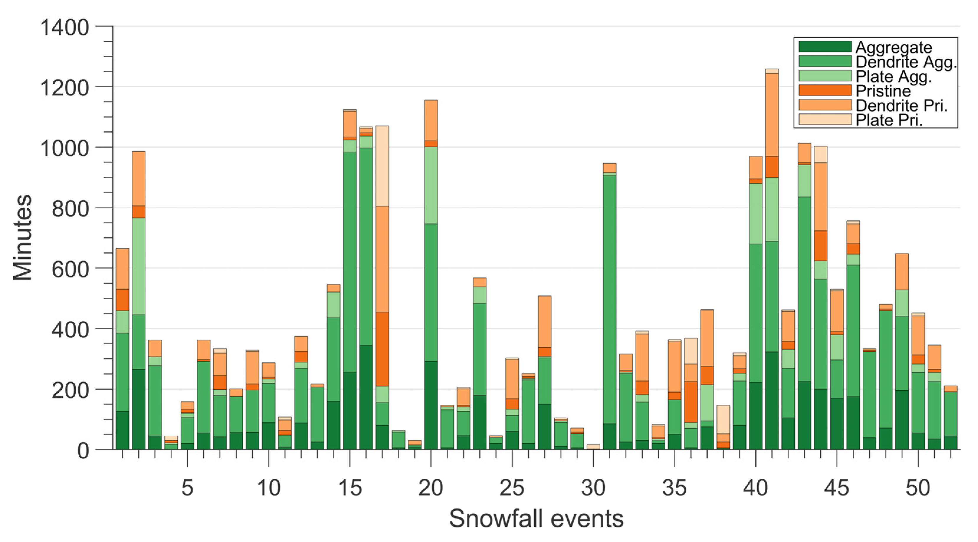
Precipitation minutes were grouped into time frames of 10 min for each of the 52 snow events. Then, the methodology described in Section 2.3 using wind-corrected Parsivel PSDs was applied for characterizing the falling particles in terms of the prevailing category. The results obtained are shown in Figure 7.

Categories of aggregates seem to better approximate the hydrometeors fallen at MZS during the periods investigated. Overall, the aggregate categories account for 17,735 min out of 23,566, with an incidence of more than 75%. In particular, the classification procedure identifies particles having specific dendrite aggregate features amounting to 45% of the total database, while 20% of the precipitation minutes are classified as belonging to the generic aggregate category. On the other hand, the categories of pristine snow seem to represent a minority (5830 min) and mainly exhibit dendrite pristine characteristics, while plate pristine appears only in 2.8% of the total minutes. However, it is worth noting that most snowfall events show a mix of the different categories, and many of them display both aggregate and pristine features. In contrast, only a single event (number 17 of 22 January 2020) consists almost solely of hydrometeors belonging to pristine-like categories. These results are consistent with other particle observations during snowfalls on the Antarctic continent, as Souverijns et al. [14] also mentioned. Such measurements indicate that precipitation events can be formed either by the coexistence of pristine and aggregate hydrometeors ([82] and references therein) or by a singular pristine habit [84].

Microphysical estimates from an X-band dual-polarization radar measurements and the high-resolution snowflake images collected by a Multiangle Snowflake Camera (MASC) performed at DDU coastal station [23] showed that aggregates account for about 40% of all falling particles, a lower percentage than that of the events observed at MZS. However, MASC identified as small particles the vast majority (56%) of the hydrometeors at the ground level due to the strong influence of blowing snow in the measurement outcomes. Moreover, results also underlined the frequent occurrence of riming particles at that site, indicating that 11% of the hydrometeors are fully rimed, and many others have a rimed degree up to 0.5 (see [85] for a detailed description). It is worth recalling that the Kuo database used in this work does not account for riming processes. Therefore, some rimed particles could not be appropriately classified. Finally, as classification is based on a comparison between instruments in terms of radar reflectivity, some large hydrometeors (aggregates) producing high Ze values could somehow hide the simultaneous presence of smaller and pristine crystals.

Density scatter plots and merit factors are again used to evaluate the classification methodology. In Figure 8, all the Ze_MRR measurements are compared with the corresponding disdrometer-derived reflectivities after applying the hydrometeor classification procedure. As we can infer from the scatter graph, the applied methodology better matches the two estimates. On the one hand, the two reflectivities result in excellent agreement for the higher Ze values and even for the most occurring range of values around 10 dBZ (red and dark-red color). However, on the other hand, the MRR observations of lower reflectivities appear to be underestimated regarding the corresponding disdrometer-derived Ze values, which can occur in weak precipitation episodes.

The corresponding improvement is also confirmed by the statistical indexes included as a text box in the figure (see Figure 4, Figure 5 and Figure 8): RMSE drops to 3.59 dBZ, while the NSE and the MD reach their minimum values. NB is slightly negative, probably related to the underestimation at lower radar Ze discussed above. Finally, the correlation coefficient rises to 0.78.

3.4. Benchmarking QPE

In each 10 min time frame, the proper Ze-SR relationship based on the classification procedure is applied to MRR measurements at the 105 m height to obtain the quantitative estimation of snow at the ground as

$$SR={\left(\frac{Ze}{a}\right)}^{\frac{1}{b}}.$$

(4)

The accumulated snowfall at MZS for the events of the Antarctic summer periods of 2018–2019 and 2019–2020 is 84.6 water equivalent mm (mm w.e.), with uncertainty between 75.4 mm and 94.8 mm w.e., expressed by means of 5th and 95th percentile of the a and b parameters.

To benchmark our outcomes, we first compare our results with other estimations obtained following different approaches, that is, using only disdrometric data or employing only radar observations coupled with literature Ze-SR relationships.

Lastly, we also compare our results with the independent estimates of accumulated snowfall from the TRwS-MPS weighing pluviometer

Accumulated snowfall values were determined using the formula for SR calculation (see Equation (3)) with wind-corrected Parsivel PSDs and different mass/velocity-diameter relationships to explore and quantify their influence in accumulation estimation. Moreover, this comparison can also highlight the extent to which a stand-alone disdrometer can return valuable estimates in snowfall without the support of co-located observations by other instruments that constrain microphysical relationships since the disdrometer does not perform any classification of the falling hydrometeors. We have used well-known mass-diameter relationships [24,86,87,88], coupled with v(D) derived from Locatelli and Hobbs [79], obtained with different methods and for different locations and particle types, to consider the natural changeableness of snow features better.

The comparison results are summarized in

Table 3. Total precipitation estimation for the considered snow episodes calculated by different methodologies and relationships, specified in the first and second column, respectively. Note that 1 and 2 in the second column indicate the use of v(D) relationships for classes of aggregates (1) or of pristines (2) derived from [79]. Differences in the last column are with respect to our snow estimation.

Method	Work (Reference Number)	Accumulated Precipitation (mm w.e.)	Difference (%)
Variable Ze-SR	Our Study	84.6 (75.4–94.8)	−
Disdrometer data, m(D) and v(D)	[86]—1	227.5	+168.9
	[86]—2	152.5	+80.3
	[87]—1	144.6	+70.9
	[87]—2	97.7	+15.5
	[88]—1	253.1	+199.2
	[88]—2	171.6	+102.8
	[24]—1	135	+59.6
	[24]—2	88.2	+4.3
Ze-SR relationship	[14]	629.2	+643.7
	[23]	74.6 (30.1–179)	−11.8
	[18]	259.4 (216.9–281.6)	+206.6

(upper rows). They show high variability in the estimation of snowfall amounts obtained using only disdrometer data. The accumulated values range between 88 and 253 mm w.e. Comparing such values to the estimate obtained using the variable Ze-SR, differences vary from a minimum of +4% to a maximum of +199%. The wide range of accumulation values indicates the dependency not only on the different mass-diameter relationships used, but also on the considered terminal speed of hydrometeors. As mass and velocity are intrinsically connected to the habit and, more broadly, to the type of snow particles, the classification of solid hydrometeors seems necessary for applying the most proper microphysical relationships in SR calculation. Otherwise, in the absence of microphysical information or constraints from distinct instruments, selecting the suited relationships could be mere guesswork.

The Ze-SR relationships developed for Antarctic sites and listed in Table 2 were employed to benchmark our methodology by applying them to MRR measurements at the 105 m height. The accumulated precipitation amounts are reported in Table 3 (lower rows). Results reflect the values of prefactors of each relationship, as expected. S17 returns the more considerable accumulation value (629.2 mm w.e.) as it is tailored for PE station, located far from the coast and with snowfall characterized by small precipitation particles and has a prefactor of 18. Instead, using the prefactor of 44 suggested in Souverijns et al. [14] for locations close to the shoreline, the amount lowers to 279 mm w.e., which is still quite far from our findings. Calculation through G17 coefficients for the DDU site (74.6 mm w.e.) seems instead to be in line with our accumulation estimates. DDU is a coastal research station that, to some extent, presents snowfall characteristics comparable to the MZS site, and, in fact, G17 was also used to compute snowfall amount at MZS (e.g., [57]).

Furthermore, we found a value of 259.4 mm w.e. making use of S20 developed for the MZS site, resulting in a difference of +206% compared to our findings and aligned with the formulas of Souverijns et al. [14] modified for coastal sites.

Some considerations arise from these results. Again, the high spread of accumulated snowfall values indicates that choosing the proper relationship to be used is fundamental. Moreover, the extreme variability of snow microphysics suggests that using a single relationship in estimating the snowfall rate appears too limited, as differences have been found not only between different sites but even among events recorded at the same location. The latter evidence also indicates that the methodology applied to achieve the Ze-SR formula can play a role in determining the a and b parameters, and, consequently, using the relationships described in the literature for SR estimations could lead to significant errors. Moreover, focusing on the MZS site, the discrepancies using S20 can also be explained not only by the differing mass-diameter parametrization but also by the different heights of the MRR measurements that can lead to quite different reflectivity measurements due to the well know sublimation mechanism acting in the lower Antarctic atmospheric levels [30].

Finally, we compared our estimates obtained with the Ze-SR mentioned above, with the Alter shield weighing gauge observations provided by the TRwS-MPS described in Section 2.1.4. This instrument was already used in the comparative analysis with snowfall amount calculated through the Ze-SR relationship in [18]. The TRwS was in operation for 32 out of 52 snow events of the analyzed period.

Figure 9 shows the comparison, in terms of accumulated snowfall values, between the weighing gauge measurements and the estimates using Ze-SR relationships, namely variable Ze-SR (as proposed in this study), S20, G17, and S17. In addition, the accumulation values contained in Scarchilli et al. [18] and calculated using S20 and the other MRR installed at MZS are also included as a further benchmark. The weighing gauge collected 31 mm w.e. in 18 snow episodes during the Antarctic summer campaign 2018–2019 and 35.5 mm w.e. during November and December 2019. The snowfall amount using variable Ze-SR relationship performs better than applying a fixed Ze-SR taken from the literature as resulting from the values closest to the reference ones in both the first and second observation period. Estimates using the G17 relationship are in line with our results, although with a slight underestimation for both periods and considerable uncertainty, while applying S20 and S17 leads to a significant overestimate. Accumulated values for the same periods, reported in Scarchilli et al. [18], are slightly larger than our estimates using variable Ze-SR and TRwS measurements, whereas they are in line considering the uncertainty. Finally, it is worth noting that the estimates using S20 and our MRR measurements are significantly larger than those in Scarchilli et al. [18], in which the S20 relationship was applied to measurements by the other MRR at MZS set with a different vertical resolution.

Although carried out in different climatic regions, several studies support the advantage of using variable Ze-SR relationships. Rasmussen et al. [25] developed an algorithm for snowfall nowcasting correlating real-time radar reflectivity and snow gauge data in the United States, deriving adaptive Ze-SR relationships. The improvement of the QPE is demonstrated because the variable Ze-SR relationship takes into account the natural variations of snow microphysics. The same conclusions can be found in von Lerber et al. [11], where the link between radar and snow properties was examined fully using measurements by video-disdrometer, pluviometer, and radar in southern Finland. It was shown that the Ze-SR relationship varies rapidly during a snowstorm, emphasizing the primary role of the prefactor value in the QPE, as also highlighted by our results. Schoger at al. [89] faced the large spread in the QPE using different Ze-SR relationships from the literature, similarly to what shown in Table 3. Applying Ze-SR relationships suited for different sites, including Antarctica, to the MRR data from Ny-Ålesund (Svalbard, Norway), they observed significant differences in snowfall rate and snowfall accumulation with respect to the reference measurements of a weighing pluviometer, ascribed to the different microphysical properties of the snow.

4. Conclusions

This work presents a new approach to quantitative snowfall estimation using a variable Ze-SR relationship based on the microphysical classification of hydrometeors. This is obtained by comparing co-located Micro Rain Radar and Parsivel disdrometer observations coupled by means of a DDA backscattering model in terms of radar reflectivity. To this end, we analyzed and processed data from 52 precipitation days at the Mario Zucchelli Italian Antarctic station collected during the 2018–2019 and 2019–2020 summer periods for a total of 23,566 observed snowfall minutes.

Before proceeding with the analysis, disdrometer data were corrected from the wind influence by a new approach that assigns a reliability weight to each Parsivel bin based on simultaneous disdrometer and wind measurements. This novelty tends to progress beyond the more used censoring method which cuts hydrometeors deviating from reference size and diameter intervals or outright eliminating precipitation data when the wind exceeds a predefined threshold that could result in heavily decimating data.

Based on these observations, we tested the consistency of Parsivel and MRR measurements based on six different snow categories and then derived the corresponding six Ze-SR relationships. The method developed can also determine the predominant snow category in each 10-min time frame for all the precipitation events. Furthermore, we applied the Ze-SR relationship of the predominant snow category to calculate the cumulated snowfall amount in the analyzed periods based on such classification. Finally, our findings were compared against estimates derived using m(D), v(D), and the Ze-SR relationships available in the literature and against co-located measurements by a weighing gauge.

The main results are as follows:

(a)

Comparisons of Ze derived from disdrometer and MRR at the 105 m height show good agreement, even for nonwind-corrected Parsivel data (Figure 4 and Figure 5, left columns), indicating the potential of the synergic use of such instrument set, despite comparing volume and point measurements but minimizing the vertical distance between the instruments;

(b)

The correspondence significantly improves using wind-corrected PSD, especially for higher reflectivity values (Figure 4 and Figure 5, right columns). Wind creates artifacts consisting mainly of a large and unusual number of tiny solid hydrometeors that corrupt PSD retrievals, leading to overestimating Ze-derived values. As strong winds usually accompany significant snow events, correction of raw disdrometric data appears mandatory in snowfall estimations, and the use of snow-reliability weight on disdrometer bins represents a valid alternative to the threshold approach in disdrometer data filtering (Figure 3);

(c)

We classified 75% of the precipitation minutes investigated at MZS as aggregate with a significant percentage of dendrites (Figure 7). Only for 5830 min out of 23,566 falling particles showed pristine characteristics. These results differ from those found at DDU (40% aggregate type). Only one snow episode is found consisting almost entirely of pristine hydrometeors and definitely deserves a closer inspection;

(d)

After hydrometeors classification, we estimated 84.6 mm w.e. of accumulated snowfall for the events observed during the summer seasons 2018–2019 and 2019–2020, using the variable Ze-SR method and benchmarked this outcome with other approaches (Table 3). We found that calculating snow amount using disdrometer data alone heavily depends on the mass and velocity parametrizations applied, resulting in a spread of precipitation accumulations ranging from 88.5 to 253.1 mm w.e. Similarly, using only MRR data and Ze-SR relationships from the literature, accumulated snowfall values lie between 74.6 and 629.2 mm w.e.;

(e)

Lastly, we have assessed our results by referencing the measures by a weighing pluviometer installed at MZS during 32 out of the 52 considered days (Figure 9). Our accumulated snow estimation from the variable Ze-SR relationship results in the best agreement (64 mm w.e. vs. 66.5 mm w.e. by the pluviometer) regarding estimates obtained with fixed Ze-SR relationships.

Because of these considerations, the combination of MRR and a disdrometer is undoubtedly valuable and workable in snowfall estimations. In contrast, disdrometer or radar data alone rely on relationships (mass-diameter and velocity-diameter for the former, Ze-SR for the latter) whose selection is not straightforward in the absence of other observations, and can lead to very different results. Their synergic use makes it possible to constrain such relationships, thanks to the precious information which can be obtained on snow microphysical features.

Moreover, the extreme variability of snow microphysical features results in significant uncertainties in snowfall estimations. Instead of a static one, the use of variable Ze-SR relationship makes it possible to mitigate the impact of such variability, as has been effectively demonstrated by the improvement in snowfall quantitative estimations.

Furthermore, our findings also warn against the simplistic (although common) use of Ze-SR relationships reported in the literature for snowfall amount computation. Since relationships are calculated with specific microphysical assumptions and are deeply tied to the instrument setting used and the methodology followed, it could be tricky to apply them to different sites and similar instrumentation with different settings. Indeed, even relationships tailored for the same site, namely MZS, can lead to different accumulated snowfall estimates.

Finally, this paper intends to propose new methodologies for the correction of disdrometer data and QPE using microphysical information through an affordable set of instruments that could give rise to advances in our knowledge of the characteristics of snowfall in Antarctica.

Although this paper presents a consistent database of 52 days of precipitation, future works are required to further validate the microphysical classification of hydrometeors employing different ground instrumentation such as imaging disdrometers to calculate accumulated snow. Additionally, it would be useful to assess the proposed methodologies during the nonsummer months.

Finally, extending further proposed approaches to other geographical contexts and sites would be interesting, especially in polar or mountainous regions.