
Fusion of UAV Hyperspectral Imaging and LiDAR for the Early Detection of EAB Stress in Ash and a New EAB Detection Index—NDVI(776,678)

 and
and
Abstract
:1. Introduction
2. Materials
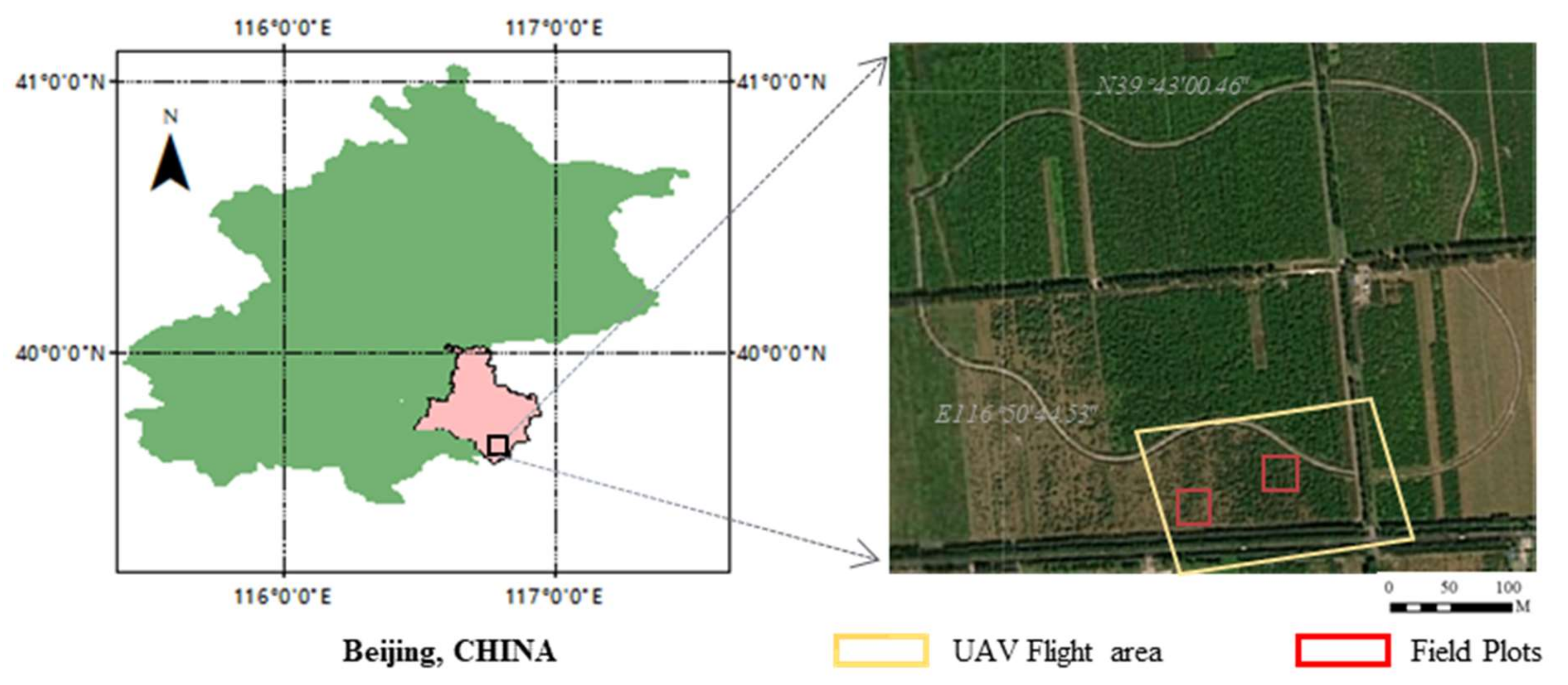
2.1. Study Area
2.2. Ground Truth data Collection
2.2.1. Chlorophyll Fluorescence
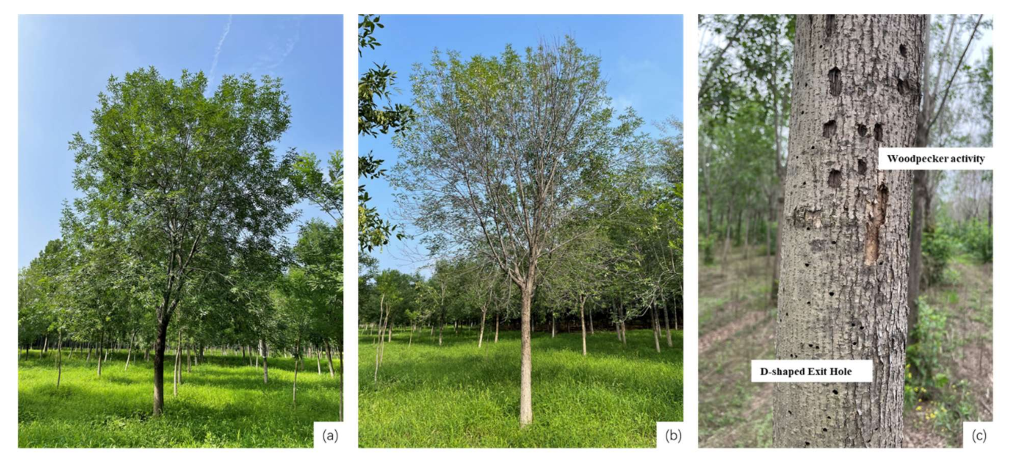
2.2.2. Crown Thinning
2.2.3. D-Shaped Exit Holes and Woodpecker Pecking Holes
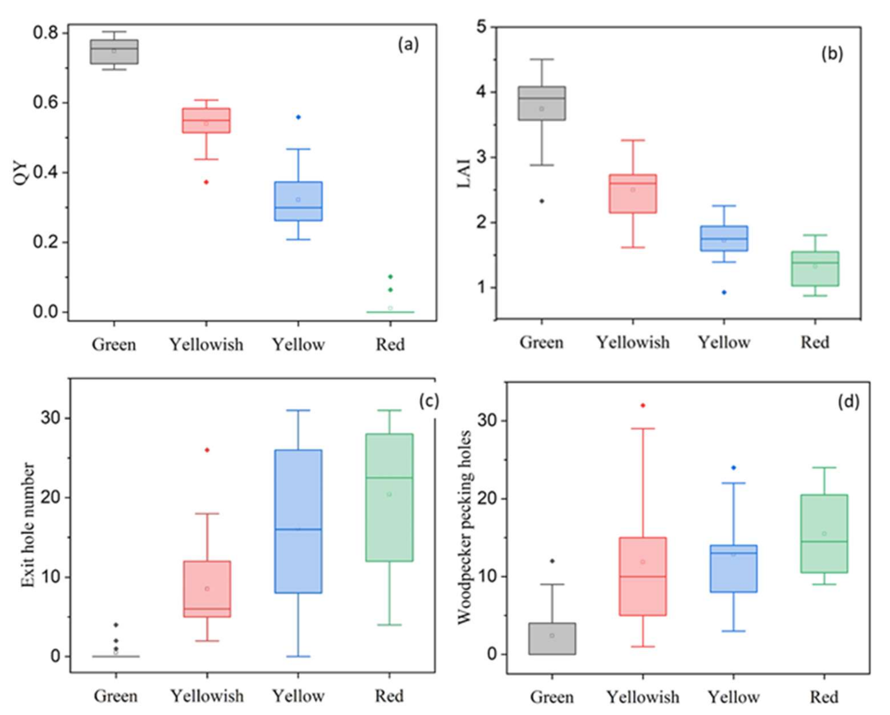
2.2.4. Canopy Color
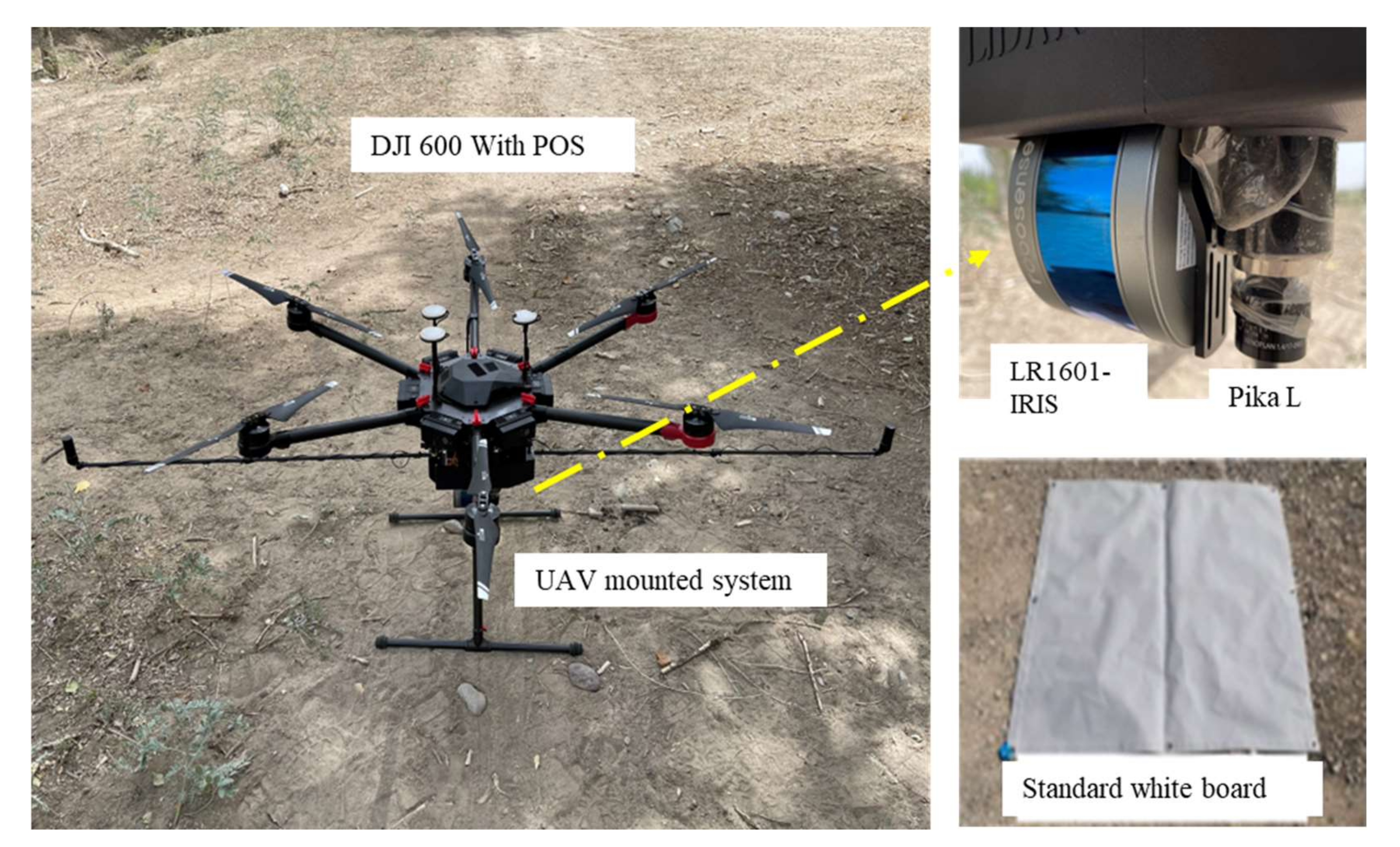
2.2.5. UAV-Based Hyperspectral Imagery and LiDAR Acquisition
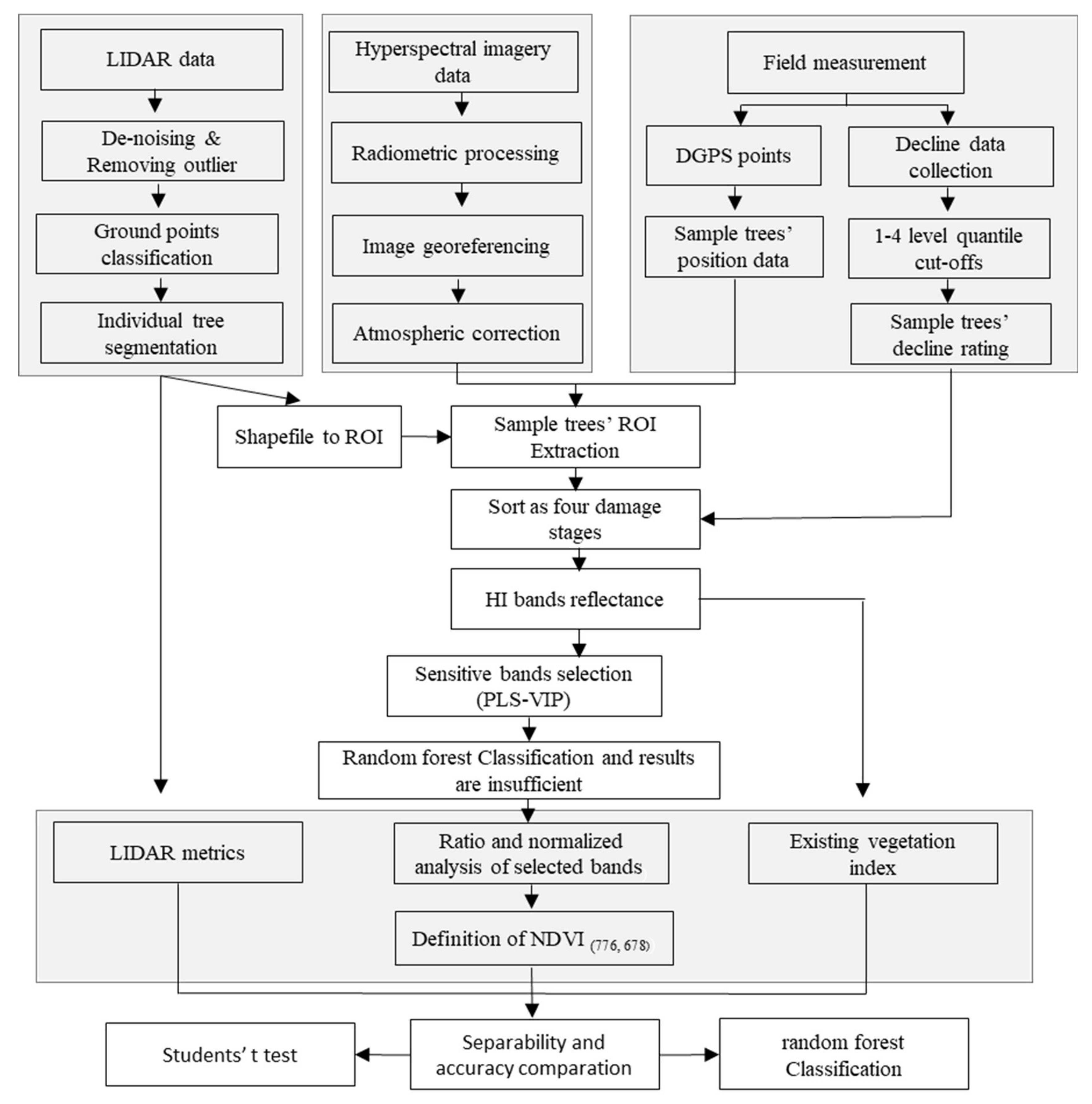
3. Methods
3.1. Individual Tree Decline Ratings
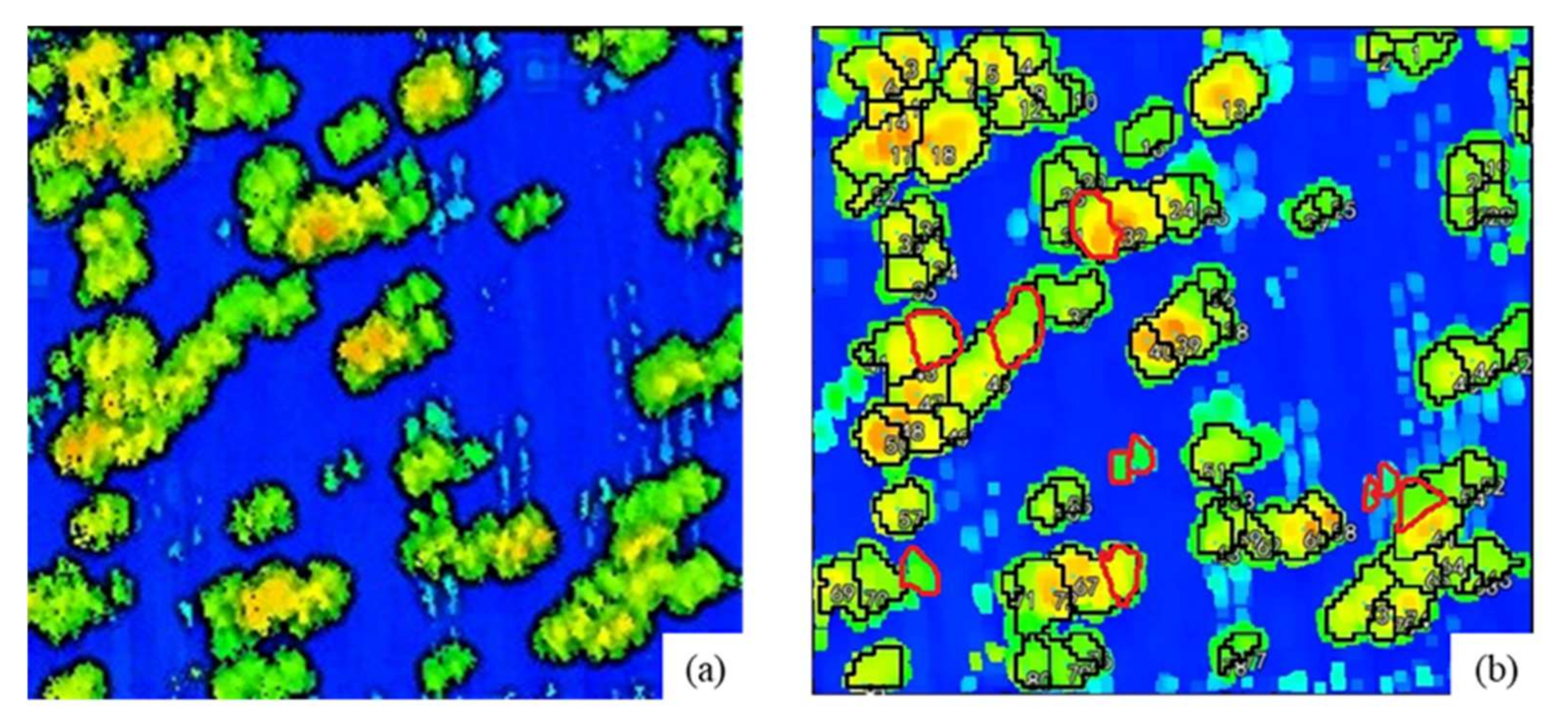
3.2. Individual Tree Segmentation and Feature Extraction
3.3. Separation of Raw Hyperspectral Bands
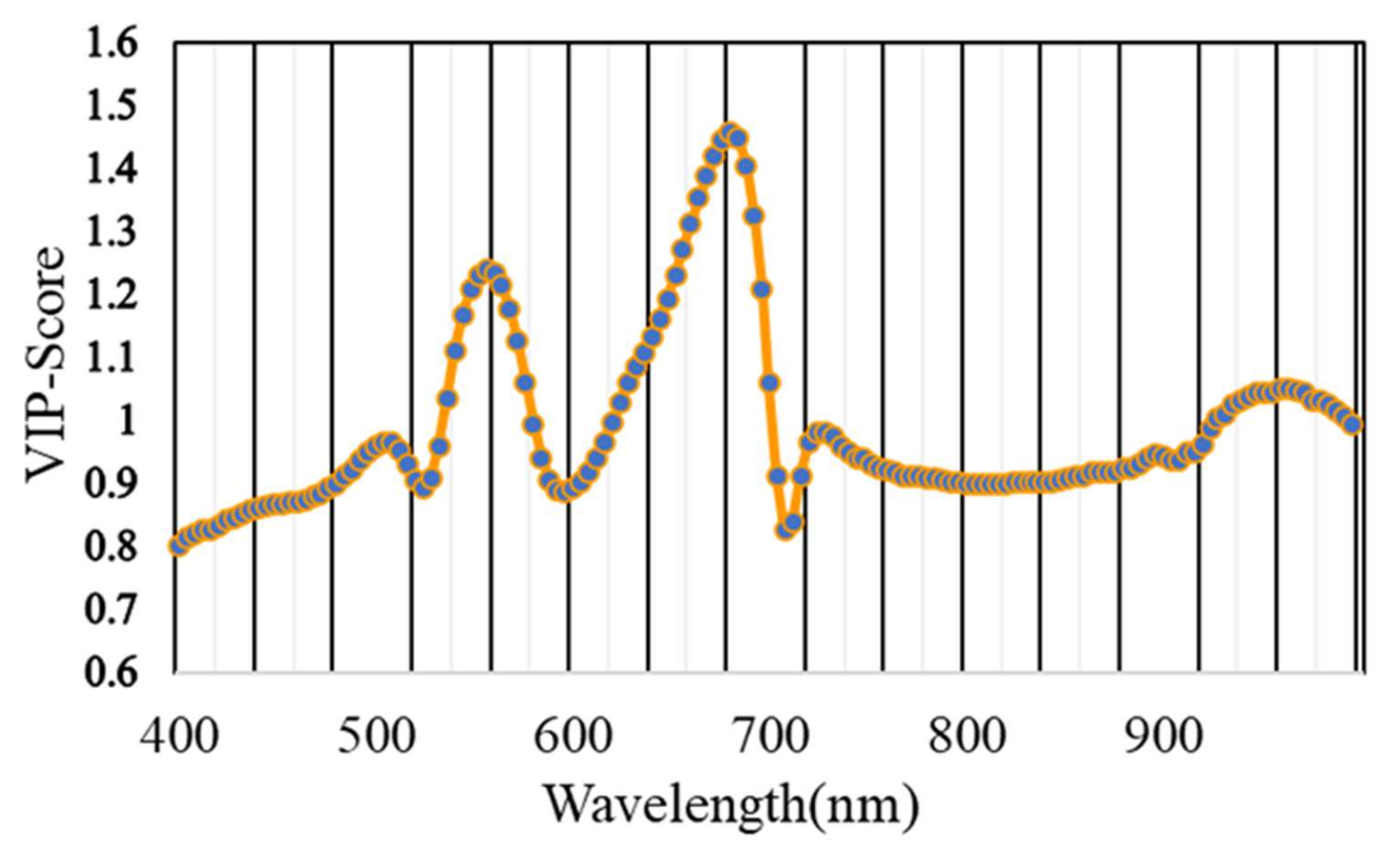
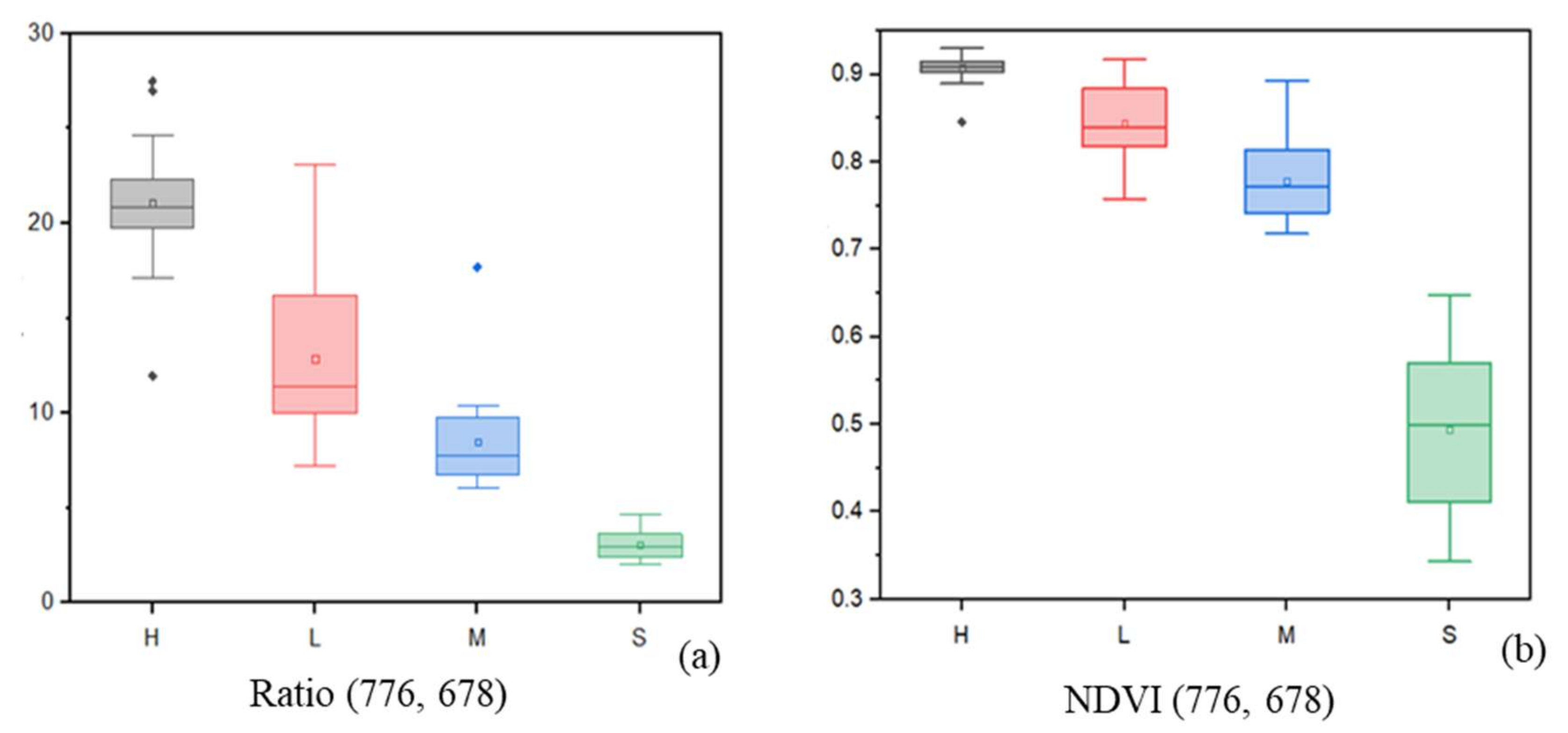
3.4. Ratio and Normalized Analysis of Sensitive Bands
3.5. Comparison with Other Vegetation Indices
4. Results
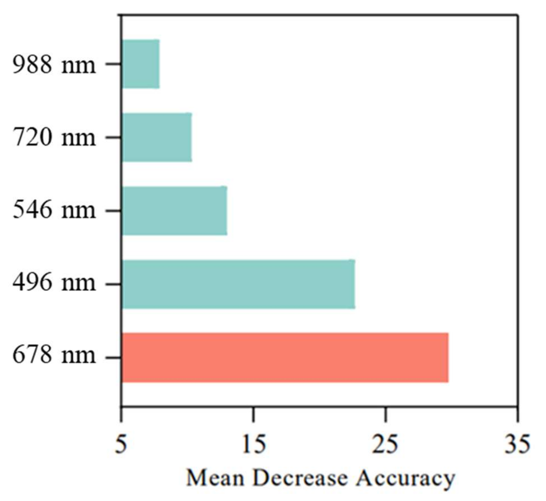
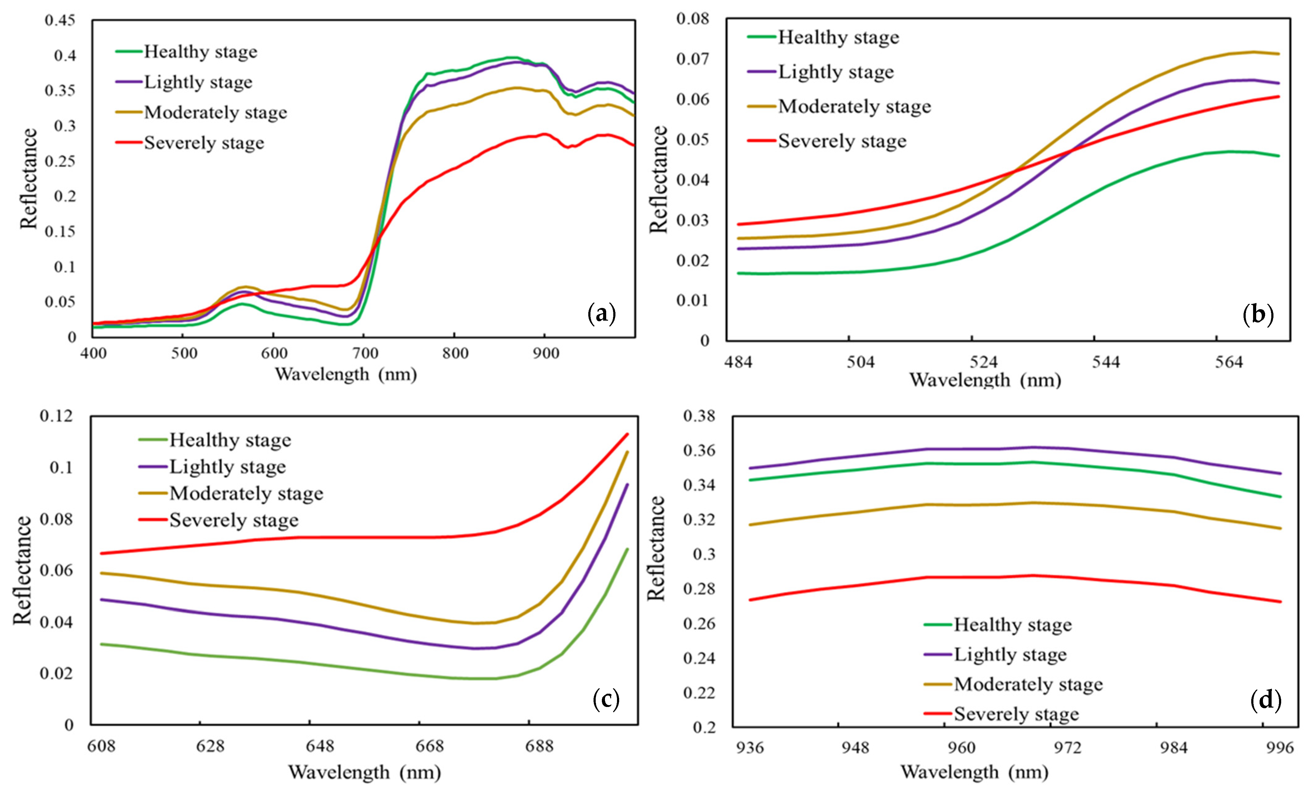
4.1. EAB-Sensitive Bands of Hyperspectral Image
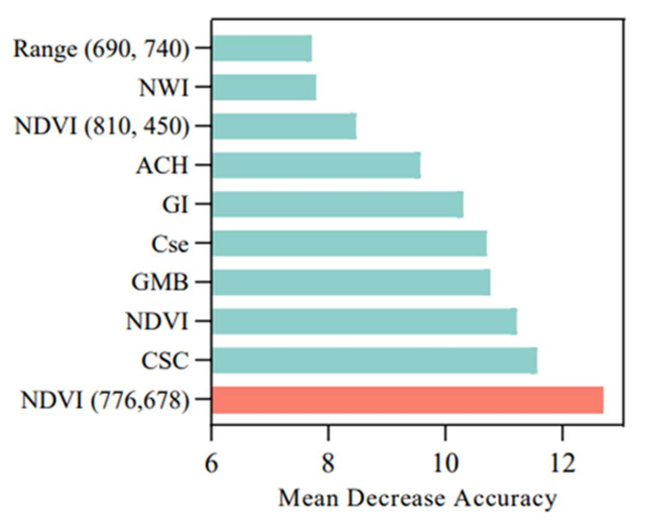
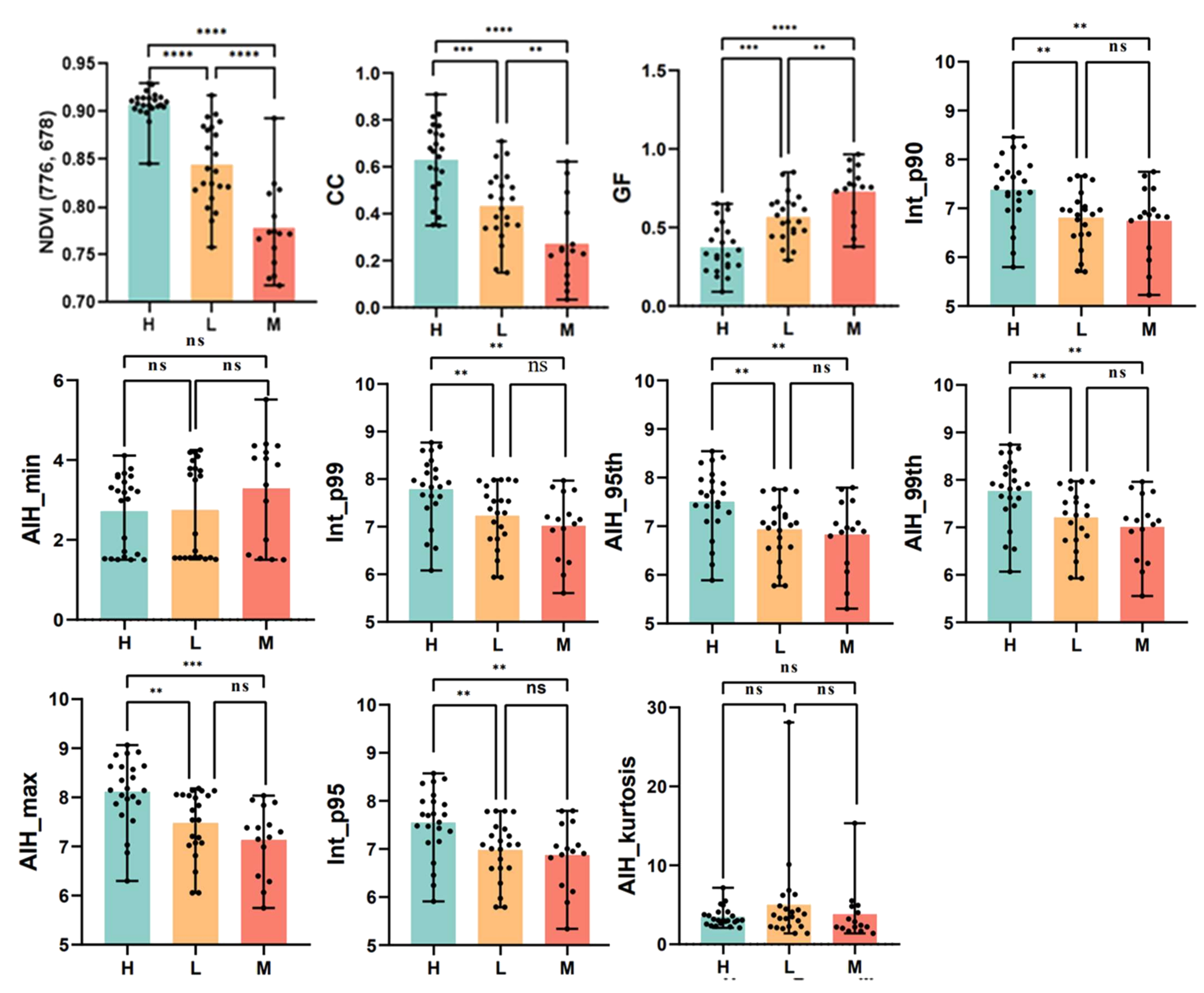
4.2. Comparison of NDVI(776,678) with Existing Vegetation Indices and LiDAR Metrics
4.3. Relationship between Canopy Color and Tree Damage
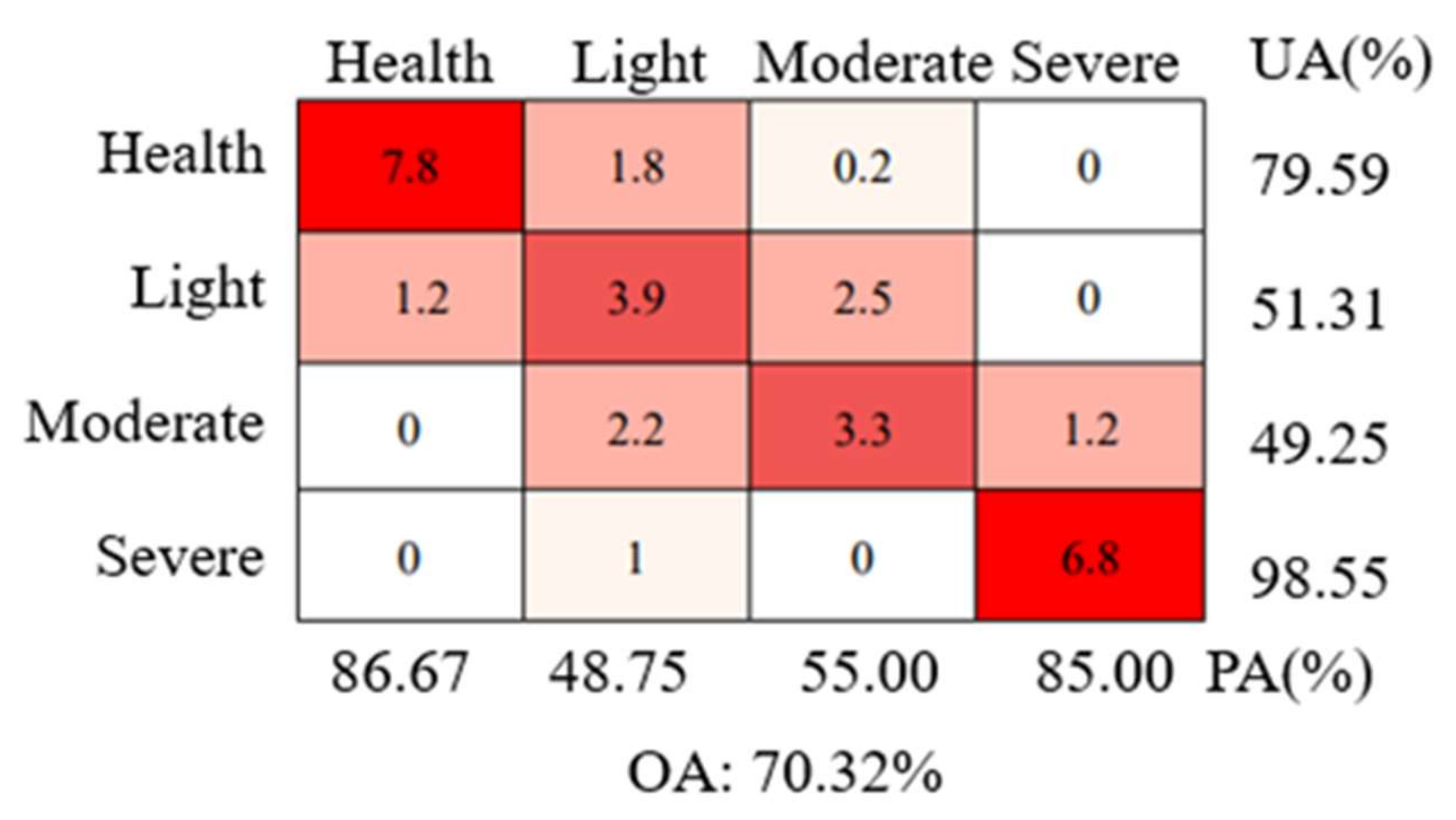
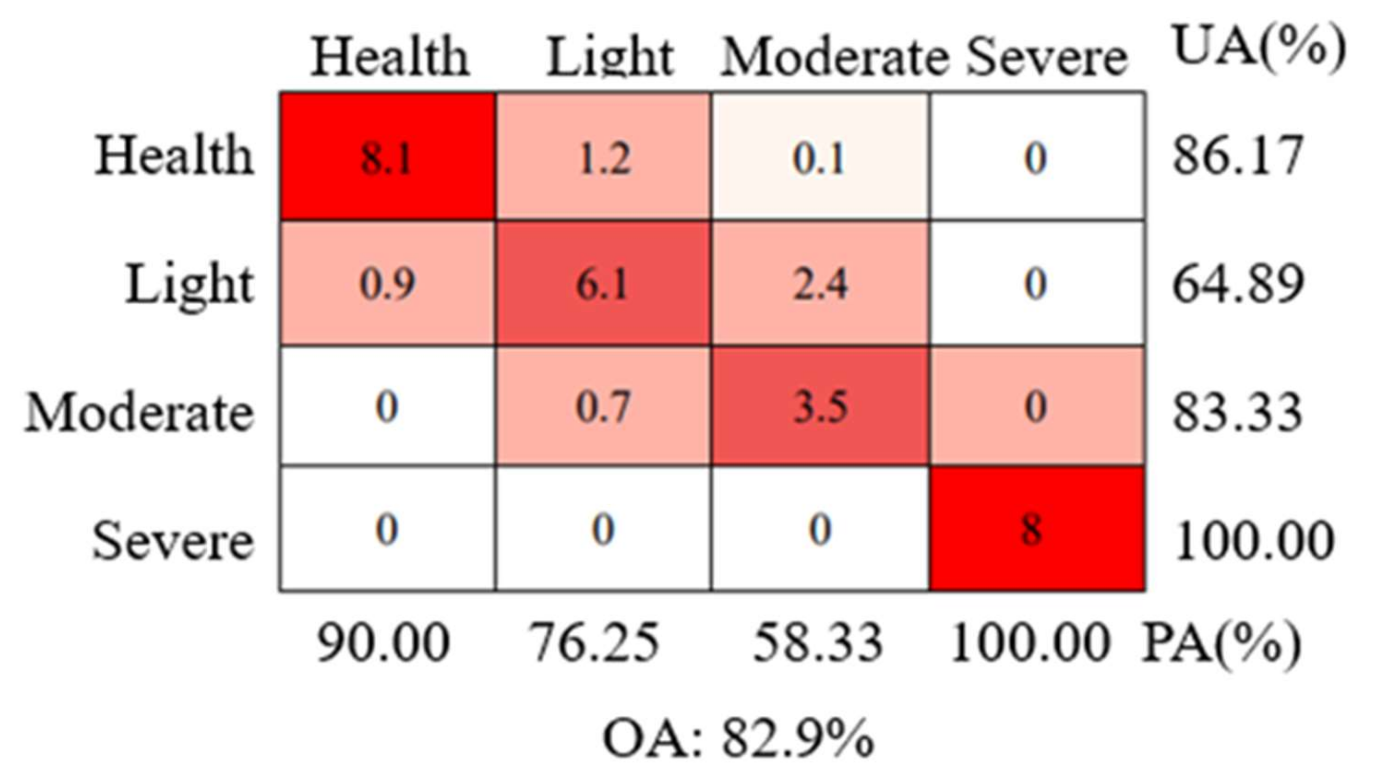
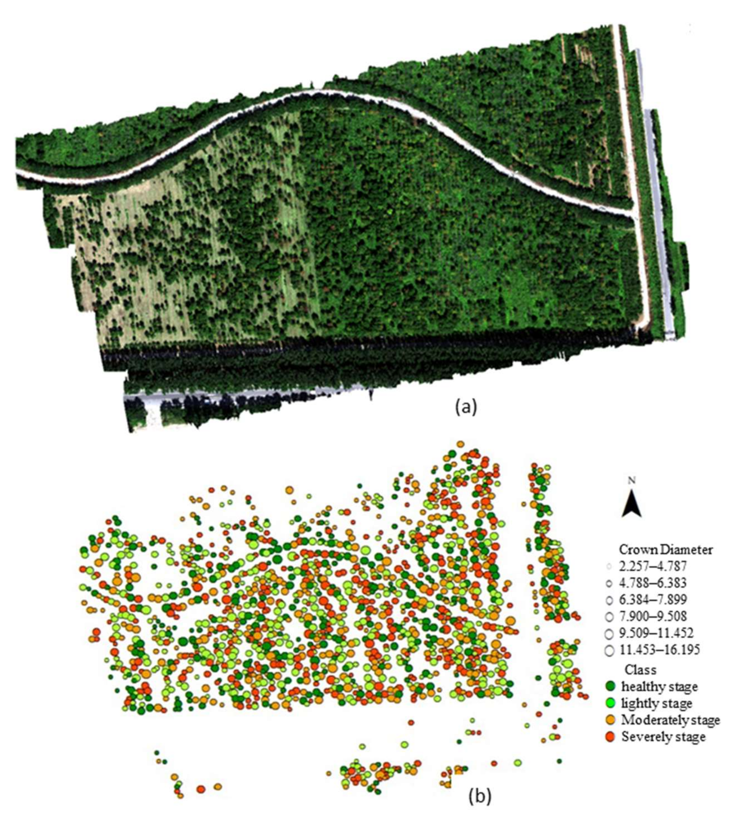
4.4. Tree Damage Mapping
5. Discussion
5.1. Remote Sensing Monitoring Window for Broad-Leaved Trees
5.2. Ash Canopy Color and Damage Stages
5.3. Method for the Early Detection of EAB
6. Conclusions
Author Contributions
Funding
Conflicts of Interest
Appendix A


References
- Maloney, K.; Boughton, J.; Schneeberger, N. Emerald Ash Borer—2006 Brief; USDA Forest Service, Northeastern Area, State and Private Forestry: Newtown Square, PA, USA, 2006. [Google Scholar]
- Siegert, N.W.; McCullough, D.G.; Liebhold, A.M.; Telewski, F.W. Spread and dispersal of emerald ash borer: A dendrochronological approach. In Proceedings of the Emerald Ash Borer Research and Technology Development Meeting, Pittsburgh, PA, USA, 26–27 September 2010; p. 10. [Google Scholar]
- Murfitt, J.; He, Y.; Yang, J.; Mui, A.; DeMille, K. Ash Decline Assessment in Emerald Ash Borer Infested Natural Forests Using High Spatial Resolution Images. Remote Sens. 2016, 8, 256. [Google Scholar] [CrossRef] [Green Version]
- McCullough, D.G.; Katovich, A.S. Emerald Ash Borer. Pest Alert; USDA Forest Service NA-PR-02-04; USDA: Newtown Square, PA, USA, 2004. [Google Scholar]
- Lee, J.E.; Frankenberg, C.; van der Tol, C.; Berry, J.A.; Guanter, L.; Boyce, C.K.; Fisher, J.B.; Morrow, E.; Worden, J.R.; Asefi, S.; et al. Forest productivity and water stress in Amazonia: Observations from GOSAT chlorophyll fluorescence. Proc. R. Soc. B Biol. Sci. 2013, 280, 20130171. [Google Scholar] [CrossRef] [PubMed] [Green Version]
- Sonobe, R.; Wang, Q. Towards a Universal Hyperspectral Index to Assess Chlorophyll Content in Deciduous Forests. Remote Sens. 2017, 9, 191. [Google Scholar] [CrossRef] [Green Version]
- Perry, S.W.; Krieg, D.R.; Hutmacher, R.B. Photosynthetic Rate Control in Cotton: Photorespiration. Plant Physiol. 1983, 73, 662–665. [Google Scholar] [CrossRef] [PubMed]
- Hicke, J.A.; Logan, J. Mapping whitebark pine mortality caused by a mountain pine beetle outbreak with high spatial resolution satellite imagery. Int. J. Remote Sens. 2009, 30, 4427–4441. [Google Scholar] [CrossRef]
- Lin, Q.; Huang, H.; Wang, J.; Huang, K.; Liu, Y. Detection of Pine Shoot Beetle (PSB) Stress on Pine Forests at Individual Tree Level using UAV-Based Hyperspectral Imagery and Lidar. Remote Sens. 2019, 11, 2540. [Google Scholar] [CrossRef] [Green Version]
- Senf, C.; Seidl, R.; Hostert, P. Remote sensing of forest insect disturbances: Current state and future directions. Int. J. Appl. Earth Obs. 2017, 60, 49–60. [Google Scholar] [CrossRef] [Green Version]
- Cheng, T.; Rivard, B.; Sánchez-Azofeifa, G.A.; Feng, J.; Calvo-Polanco, M. Continuous wavelet analysis for the detection of green attack damage due to mountain pine beetle infestation. Remote Sens. Environ. 2010, 114, 899–910. [Google Scholar] [CrossRef]
- Tang, L.; Shao, G. Drone remote sensing for forestry research and practices. J. For. Res. 2015, 26, 791–797. [Google Scholar] [CrossRef]
- Hoque, E.; Hutzler, P.J.S. Spectral blue-shift of red edge minitors damage class of beech trees. Remote Sens. Environ. 1992, 39, 81–84. [Google Scholar] [CrossRef]
- Carter, G.A.; Knapp, A.K. Leaf optical properties in higher plants: Linking spectral characteristics to stress and chlorophyll concentration. Am. J. Bot. 2001, 88, 677–684. [Google Scholar] [CrossRef] [PubMed] [Green Version]
- Yu, R.; Luo, Y.; Zhou, Q.; Zhang, X.; Ren, L. A machine learning algorithm to detect pine wilt disease using UAV-based hyperspectral imagery and LiDAR data at the tree level. Int. J. Appl. Earth Obs. Geoinf. 2021, 101, 102363. [Google Scholar] [CrossRef]
- Lambert, J.; Denux, J.-P.; Verbesselt, J.; Balent, G.; Cheret, V. Detecting Clear-Cuts and Decreases in Forest Vitality Using MODIS NDVI Time Series. Remote Sens. 2015, 7, 3588–3612. [Google Scholar] [CrossRef] [Green Version]
- Recanatesi, F.; Giuliani, C.; Ripa, M. Monitoring Mediterranean Oak Decline in a Peri-Urban Protected Area Using the NDVI and Sentinel-2 Images: The Case Study of Castelporziano State Natural Reserve. Sustainability 2018, 10, 3308. [Google Scholar] [CrossRef] [Green Version]
- Peddle, D.R.; Boulton, R.B.; Pilger, N.; Bergeron, M.; Hollinger, A. Hyperspectral detection of chemical vegetation stress: Evaluation for the Canadian HERO satellite mission. Can. J. Remote Sens. 2008, 34, S198–S216. [Google Scholar] [CrossRef]
- Dechesne, C.; Mallet, C.; Le Bris, A.; Gouet-Brunet, V. How to combine lidar and very high resolution multispectral images for forest stand segmentation? In Proceedings of the 2017 IEEE International Geoscience and Remote Sensing Symposium (IGARSS), Fort Worth, TX, USA, 23–28 July 2017. [CrossRef]
- Awad, M.M. Toward Robust Segmentation Results Based on Fusion Methods for Very High Resolution Optical Image and LiDAR Data. IEEE J. Sel. Top. Appl. Earth Obs. Remote Sens. 2017, 10, 2067–2076. [Google Scholar] [CrossRef]
- Reyes-Palomeque, G.; Dupuy, J.M.; Johnson, K.D.; Castillo-Santiago, M.A.; Hernández-Stefanoni, J.L. Combining LiDAR data and airborne imagery of very high resolution to improve aboveground biomass estimates in tropical dry forests. Forestry 2019, 92, 599–615. [Google Scholar] [CrossRef]
- Wang, J.; Feng, J.; Yan, Z. Impact of Extensive Urbanization on Summertime Rainfall in the Beijing Region and the Role of Local Precipitation Recycling. J. Geophys. Res. Atmos. 2018, 123, 3323–3340. [Google Scholar] [CrossRef]
- Liu, W.; You, H.; Dou, J. Urban-rural humidity and temperature differences in the Beijing area. Theor. Appl. Climatol. 2008, 96, 201–207. [Google Scholar] [CrossRef]
- Teskey, R.O.; Gholz, H.L.; Cropper, W.P. Influence of climate and fertilization on net photosynthesis of mature slash pine. Tree Physiol. 1994, 14, 1215–1227. [Google Scholar] [CrossRef]
- Janka, E.; Körner, O.; Rosenqvist, E.; Ottosen, C.O. Using the quantum yields of photosystem II and the rate of net photosynthesis to monitor high irradiance and temperature stress in chrysanthemum (Dendranthema grandiflora). Plant Physiol. Biochem. 2015, 90, 14–22. [Google Scholar] [CrossRef] [PubMed]
- Hernández-Clemente, R.; North, P.R.J.; Hornero, A.; Zarco-Tejada, P.J. Assessing the effects of forest health on sun-induced chlorophyll fluorescence using the FluorFLIGHT 3-D radiative transfer model to account for forest structure. Remote Sens. Environ. 2017, 193, 165–179. [Google Scholar] [CrossRef] [Green Version]
- Smitley, D.; Davis, T.; Rebek, E. Progression of ash canopy thinning and dieback outward from the initial infestation of emerald ash borer (Coleoptera: Buprestidae) in southeastern Michigan. J. Econ. Entomol. 2008, 101, 1643–1650. [Google Scholar] [CrossRef] [PubMed]
- Liu, Y.; Liu, R.; Chen, J.; Cheng, X.; Zheng, G. Current status and perspectives of leaf area index retrieval from optical remote sensing data. J. Geo-Inf. Sci. 2013, 15, 734–743. (In Chinese) [Google Scholar] [CrossRef]
- Orlando, F.; Movedi, E.; Paleari, L.; Gilardelli, C.; Foi, M.; Dell’Oro, M.; Confalonieri, R. Estimating leaf area index in tree species using the PocketLAI smartapp. Appl. Veg. Sci. 2015, 18, 716–723. [Google Scholar] [CrossRef]
- Herms, D.A.; McCullough, D.G. Emerald ash borer invasion of North America: History, biology, ecology, impacts, and management. Annu. Rev. Entomol. 2014, 59, 13–30. [Google Scholar] [CrossRef] [PubMed] [Green Version]
- Pontius, J.; Martin, M.; Plourde, L.; Hallett, R. Ash decline assessment in emerald ash borer-infested regions: A test of tree-level, hyperspectral technologies. Remote Sens. Environ. 2008, 112, 2665–2676. [Google Scholar] [CrossRef]
- Chen, Q.; Baldocchi, D.; Gong, P.; Kelly, M. Isolating Individual Trees in a Savanna Woodland Using Small Footprint Lidar Data. Photogramm. Eng. Remote Sens. 2006, 72, 923–932. [Google Scholar] [CrossRef] [Green Version]
- Zhao, D.; Pang, Y.; Li, Z.; Sun, G. Filling invalid values in a lidar-derived canopy height model with morphological crown control. Int. J. Remote Sens. 2013, 34, 4636–4654. [Google Scholar] [CrossRef]
- Savitzky, A.; Golay, M.J.E. Smoothing and Differentiation of Data by Simplified Least Squares Procedures. Anal. Chem. 1964, 6, 1627–1639. [Google Scholar] [CrossRef]
- Kubinyi, H. 3D Qsar in Drug Design: Theory, Methods and Applications; Springer Science & Business Media: Berlin/Heidelberg, Germany, 1993. [Google Scholar]
- Chong, I.; Chi-hyuck, J. Performance of some variable selection methods when multicollinearity is present. Chemom. Intell. Lab. Syst. 2005, 78, 103–112. [Google Scholar] [CrossRef]
- Breiman, L. Random forests. Mach. Learn. 2001, 45, 5–32. [Google Scholar] [CrossRef] [Green Version]
- Waske, B.; Benediktsson, J.A.; Árnason, K.; Sveinsson, J.R. Mapping of hyperspectral AVIRIS data using machine-learning algorithms. Can. J. Remote Sens. 2009, 35, 106–116. [Google Scholar] [CrossRef]
- Liu, L.; Coops, N.C.; Aven, N.W.; Pang, Y. Mapping urban tree species using integrated airborne hyperspectral and lidar remote sensing data. Remote Sens. Environ. 2017, 200, 170–182. [Google Scholar] [CrossRef]
- Carter, G.A. Ratios of leaf reflectances in narrow wavebands as indicators of plant stress. Int. J. Remote Sens. 1994, 15, 697–703. [Google Scholar] [CrossRef]
- Rouse, J.W.J.; Haas, R.H.; Schell, J.A.; Deering, D.W. Monitoring Vegetation Systems in the Great Plains with ERTS. NASA Spec. Publ. 1974, 1, 309–317. [Google Scholar]
- Carter, G.A.; Miller, M.L. Early detection of plant stress by digital imaging within narrow stress-sensitive wavebands. Remote Sens. Environ. 1994, 50, 295–302. [Google Scholar] [CrossRef]
- Gitelson, A.A.; Merzlyak, M.N. Quantitative estimation of chlorophyll-a using reflectance spectra: Experiments with autumn chestnut and maple leaves. J. Photochem. Photobiol. 1994, 22, 247–252. [Google Scholar] [CrossRef]
- Shi, Y.; Wang, T.; Skidmore, A.K.; Heurich, M. Important lidar metrics for discriminating forest tree species in Central Europe. ISPRS J. Photogramm. Remote Sens. 2018, 137, 163–174. [Google Scholar] [CrossRef]
- Smith, R.C.G.; Adams, J.; Stephens, D.J.; Hick, P.T. Forecasting wheat yield in a Mediterranean-type environment from the NOAA satellite. Aust. J. Agric. Res. 1995, 46, 113. [Google Scholar] [CrossRef]
- Barnes, J.D.; Balaguer, L.; Manrique, E.; Elvira, S.; Davison, A.W. A reappraisal of the use of DMSO for the extraction and determination of chlorophylls a and b in lichens and higher plants. Environ. Exp. Bot. 1992, 32, 85–100. [Google Scholar] [CrossRef]
- Carter, G.A. Responses of leaf spectral reflectance to plant stress. Am. J. Bot. 1993, 80, 239–243. [Google Scholar] [CrossRef]
- Gamon, J.A.; Surfus, J.S. Assessing leaf pigment content and activity with a reflectometer. New Phytol. 1999, 143, 105–117. [Google Scholar] [CrossRef]
- Babar, M.A.; Reynolds, M.P.; van Ginkel, M.; Klatt, A.R.; Raun, W.R.; Stone, M.L. Spectral Reflectance Indices as a Potential Indirect Selection Criteria for Wheat Yield under Irrigation. Crop Sci. 2006, 46, 578–588. [Google Scholar] [CrossRef]
- Richardson, A.J.; Wiegand, C.L. Distinguishing vegetation from soil background information. Photogramm. Eng. Remote Sens. 1977, 43, 1541–1552. [Google Scholar]
- Merton, R.N. Multi-Temporal Analysis of Community Scale Vegetation Stress with Imaging Spectroscopy. Ph.D. Thesis, University of Auckland, Auckland, New Zealand, 1999. [Google Scholar]
- Shendryk, I.; Broich, M.; Tulbure, M.G.; McGrath, A.; Keith, D.; Alexandrov, S.V. Mapping individual tree health using full-waveform airborne laser scans and imaging spectroscopy: A case study for a floodplain eucalypt forest. Remote Sens. Environ. 2016, 187, 202–217. [Google Scholar] [CrossRef]


| Decline Ratings Quantile | Measured QY | LAI | Number of Exit Holes | Number of Woodpecker Feeding Holes |
|---|---|---|---|---|
| 4 | 0.606–0.85 | 2.88–4.51 | 0–4 | 0–3 |
| 3 | 0.493–0.605 | 2.11–2.87 | 5–10 | 4–9 |
| 2 | 0.158–0.492 | 1.62–2.10 | 11–18 | 10–16 |
| 1 | 0–0.157 | 0–1.61 | 19–31 | 17–32 |
| Damage Stage | Average Tree Decline Rating Value |
|---|---|
| Healthy (H) | 3.17–4 |
| Light (L) | 2.39–3.16 |
| Moderate (M) | 1.39–2.38 |
| Severe (S) | 1–1.38 |
| Variables | Formula | Reference |
|---|---|---|
| CSC | R605/R760 | [42] |
| GI | R554/R677 | [45] |
| NPQI | (R415 − R435)/(R415 + R435) | [46] |
| GMB | R750/R700 | [43] |
| WBI | R970/R900 | [47] |
| ACH | SUM(R600:R700)/SUM(R500:R600) | [48] |
| NWI | (R970 − R850)/(R970 + R850) | [49] |
| Cse | R605/R760 | [42] |
| NDVI | (R800 − R670)/(R800 + R670) | [41] |
| NDVI(810,450) | (R810 − R450)/(R810 + R450) | [50] |
| Range (690, 740) | MAX(R690:R740) − MIN(R690:R740) | [51] |
| Metrics | Definition |
|---|---|
| CC | Canopy cover |
| GF | Gap fraction |
| AIH_99th | Accumulate interquartile height of 99th |
| AIH_95th | Accumulate interquartile height of 95th |
| AIH_kurtosis | Kurtosis of accumulate interquartile height |
| AIH_max | Maximum point cloud height |
| AIH_min | Maximum point cloud height |
| Int_p90 | 90th percentile of crown return intensity |
| Int_p95 | 95th percentile of crown return intensity |
| Int_p99 | 99th percentile of crown return intensity |
| Model | Healthy | Lightly | Moderately | Severely | All Stages | |||||
|---|---|---|---|---|---|---|---|---|---|---|
| UA (%) | PA (%) | UA (%) | PA (%) | UA (%) | PA (%) | UA (%) | PA (%) | OA (%) | ||
| Include NDVI(776,678) | HI + LIDAR | 86.17 | 90.00 | 64.89 | 76.25 | 83.33 | 58.33 | 100 | 100 | 82.90 |
| HI | 84.04 | 87.78 | 56.67 | 68.92 | 76.09 | 53.03 | 100 | 100 | 79.03 | |
| LIDAR | 82.22 | 68.51 | 48.00 | 60.00 | 46.42 | 43.33 | 74.47 | 72.92 | 70.32 | |
| Exclude NDVI(776,678) | HI + LIDAR | 81.19 | 91.11 | 59.76 | 61.25 | 76.92 | 61.54 | 100 | 100 | 79.68 |
| HI | 75.24 | 87.78 | 53.83 | 52.50 | 73.33 | 56.90 | 100 | 100 | 75.97 | |
| LIDAR | 66.67 | 83.33 | 30.56 | 34.38 | 30.00 | 12.50 | 54.55 | 56.25 | 50.00 | |
Publisher’s Note: MDPI stays neutral with regard to jurisdictional claims in published maps and institutional affiliations. |
© 2022 by the authors. Licensee MDPI, Basel, Switzerland. This article is an open access article distributed under the terms and conditions of the Creative Commons Attribution (CC BY) license (https://creativecommons.org/licenses/by/4.0/).
Share and Cite
Zhou, Q.; Yu, L.; Zhang, X.; Liu, Y.; Zhan, Z.; Ren, L.; Luo, Y. Fusion of UAV Hyperspectral Imaging and LiDAR for the Early Detection of EAB Stress in Ash and a New EAB Detection Index—NDVI(776,678). Remote Sens. 2022, 14, 2428. https://doi.org/10.3390/rs14102428
Zhou Q, Yu L, Zhang X, Liu Y, Zhan Z, Ren L, Luo Y. Fusion of UAV Hyperspectral Imaging and LiDAR for the Early Detection of EAB Stress in Ash and a New EAB Detection Index—NDVI(776,678). Remote Sensing. 2022; 14(10):2428. https://doi.org/10.3390/rs14102428
Chicago/Turabian StyleZhou, Quan, Linfeng Yu, Xudong Zhang, Yujie Liu, Zhongyi Zhan, Lili Ren, and Youqing Luo. 2022. "Fusion of UAV Hyperspectral Imaging and LiDAR for the Early Detection of EAB Stress in Ash and a New EAB Detection Index—NDVI(776,678)" Remote Sensing 14, no. 10: 2428. https://doi.org/10.3390/rs14102428