
Impact of the Dates of Input Image Pairs on Spatio-Temporal Fusion for Time Series with Different Temporal Variation Patterns


1
State Key Laboratory of Remote Sensing Science, Faculty of Geographical Science, Beijing Normal University, Beijing 100875, China
2
Beijing Engineering Research Center for Global Land Remote Sensing Products, Institute of Remote Sensing Science and Engineering, Faculty of Geographical Science, Beijing Normal University, Beijing 100875, China
*
Author to whom correspondence should be addressed.
Remote Sens. 2022, 14(10), 2431; https://doi.org/10.3390/rs14102431
Submission received: 17 March 2022
/
Revised: 24 April 2022
/
Accepted: 17 May 2022
/
Published: 19 May 2022
(This article belongs to the Special Issue Multi-Sensor Data Fusion and Analysis of Multi-Temporal Remotely Sensed Imagery II)
Abstract
:Dense time series of remote sensing images with high spatio-temporal resolution are critical for monitoring land surface dynamics in heterogeneous landscapes. Spatio-temporal fusion is an effective solution to obtaining such time series images. Many spatio-temporal fusion methods have been developed for producing high spatial resolution images at frequent intervals by blending fine spatial images and coarse spatial resolution images. Previous studies have revealed that the accuracy of fused images depends not only on the fusion algorithm, but also on the input image pairs being used. However, the impact of input images dates on the fusion accuracy for time series with different temporal variation patterns remains unknown. In this paper, the impact of input image pairs on the fusion accuracy for monotonic linear change (MLC), monotonic non-linear change (MNLC), and non-monotonic change (NMC) time periods were evaluated, respectively, and the optimal selection strategies of input image dates for different situations were proposed. The 16-day composited NDVI time series (i.e., Collection 6 MODIS NDVI product) were used to present the temporal variation patterns of land surfaces in the study areas. To obtain sufficient observation dates to evaluate the impact of input image pairs on the spatio-temporal fusion accuracy, we utilized the Harmonized Landsat-8 Sentinel-2 (HLS) data. The ESTARFM was selected as the spatio-temporal fusion method for this study. The results show that the impact of input image date on the accuracy of spatio-temporal fusion varies with the temporal variation patterns of the time periods being fused. For the MLC period, the fusion accuracy at the prediction date (PD) is linearly correlated to the time interval between the change date (CD) of the input image and the PD, but the impact of the input image date on the fusion accuracy at the PD is not very significant. For the MNLC period, the fusion accuracy at the PD is non-linearly correlated to the time interval between the CD and the PD, the impact of the time interval between the CD and the PD on the fusion accuracy is more significant for the MNLC than for the MLC periods. Given the similar change of time intervals between the CD and the PD, the increments of R2 of fusion result for the MNLC is over ten times larger than those for the MLC. For the NMC period, a shorter time interval between the CD and the PD does not lead to higher fusion accuracies. On the contrary, it may lower the fusion accuracy. This study suggests that temporal variation patterns of the data must be taken into account when selecting optimal dates of input images in the fusion model.
1. Introduction
Spatial and temporal resolution are the fundamental and key issues in the field of remote sensing. In recent years, a large number of satellite sensors with different spatial, temporal, and spectral characteristics have been launched, resulting in a dramatic improvement in the ability of obtaining images of the Earth’s surface [1]. Many satellite data sets such as MODIS, Landsat, and Sentinel-2 images became available to the public free of charge [2,3]. However, these sensors typically represent a trade-off between spatial and temporal resolution due to technical and financial constraints [4,5], which makes obtaining images with both a high temporal and spatial resolution a challenge [6]. For example, Landsat acquires images with a relatively high spatial resolution (30 m), but with a low temporal resolution (a 16-day revisit period), while Moderate Resolution Imaging Spectroradiometer (MODIS) acquires images with a coarse spatial resolution (250 m in red and NIR bands and 500 m in other land reflectance bands) but with a high temporal resolution (daily). Dense time series remote sensing images with both high spatial and temporal resolutions are highly desired for land cover mapping [7], forest disturbance monitoring [8], carbon sequestration modeling [9], crop yields estimation [10,11], understanding human–nature interactions [12], and revealing the ecosystem–climate feedback [13]. Spatio-temporal fusion of multi-source remote sensing images is an effective approach to obtaining high spatial and temporal resolution data [14].
Spatio-temporal fusion is an approach for fusing satellite images from two sensors with a high temporal resolution but a coarse spatial resolution (e.g., MODIS) and a high spatial resolution but a low temporal resolution (e.g., Landsat and Sentinel-2A/B) [15]. The output of spatio-temporal fusion is a synthesized image with both a high spatial and temporal resolution. Spatio-temporal fusion algorithms have been developed rapidly over the past decade [16]. Among them, the most cited method is the STARFM [6], which used a pair of Landsat and MODIS images collected on the same date to predict the Landsat scale reflectance at other MODIS image dates.
The STARFM has been widely used and became the basis for many other methods, such as the STAARCH [17], the semi-physical fusion approach [18], and the ESTARFM [19]. Building upon the STARFM by introducing a conversion coefficient and using two image pairs to select similar pixels [20,21], the ESTARFM with the improved accuracy in heterogeneous areas has become the most widely used spatio-temporal fusion algorithm.
Previous studies demonstrated that in addition to the fusion algorithms, the accuracy of spatio-temporal fusion also highly depends on the selection of the base image pairs [22,23]. Considerable efforts have been made to evaluate the influence of input image pairs on the accuracy of spatio-temporal fusion [24]. Zhu et al. [25] selected the base image pair that was temporally nearest to the prediction date for spatio-temporal fusion. This is called the nearest date strategy (NDS). However, selecting the input image pairs closest to the prediction date does not ensure the highest fusion accuracy [22]. Essentially, the spatio-temporal fusion accuracy is largely dependent on the similarity between pixels of the input image and those at the prediction date, and the similarity is affected by many factors such as land cover changes [24], radiometric differences [26,27], and the time interval between the input image date and the prediction date [19]. Xie et al. [24] suggested that the correlation of the images between the base and prediction dates can be used to express the similarity of those images, and thereby proposed the highest correlation strategy (HCS) for selecting input image pairs. They further demonstrated that the spatio-temporal fusion accuracy based on HCS outperforms that of the NDS for the STARFM [24]. Building upon previous works, Wang et al. [22] proposed an operational fusion framework in which the user can make a choice between the NDS and HCS. Alternatively, Chen et al. [28] proposed a cross-fusion method that considers the radiometric differences between the images of base and prediction dates.
As we note above, the impact of the similarity between the images of input pair to the one at the prediction date on the fusion accuracy has been broadly recognized. However, the relationship between the similarity and time interval of two images on two dates is complex and demands in-depth investigation. The similarity between the input image pair to the prediction date also depends on the temporal variation patterns of the variables being fused (e.g., surface reflectance and NDVI). The temporal variation of pixels can have different patterns such as the monotonic linear, the monotonic non-linear, and the non-monotonic. For the different temporal variation patterns, the similarity between the input image pair to the prediction date would be different, even when the time interval between the input images and the prediction date is the same. However, the impacts of temporal variation patterns on the accuracy of spatio-temporal fusion have not yet been investigated. Thus, the impact of input image dates on the accuracy of spatio-temporal fusion for land surface with different temporal variations remains unknown. To address this gap, this study aims to investigate the impacts of the input image pair on the spatio-temporal fusion accuracy for the time series with different temporal variation patterns. The ultimate goal is to provide new insights for the optimal selection of input data to increase accuracies in the spatio-temporal fusion model.
2. Data and Study Area
2.1. Satellite Data
2.1.1. Fine Spatial Resolution Data
To analyze the impacts of dates of input images on the fusion accuracy of variables with different temporal variation patterns, dense high spatial resolution images are required. Due to the limitation of revisit period and cloud cover [29,30], images acquired by a single satellite sensor such as Landsat are temporally sparse [31,32]. To obtain a sufficient number of high spatial resolution images, in this study, the HLS (Harmonized Landsat-8 Sentinel-2) product (version 1.4) was used as the fine resolution input images for spatio-temporal fusion (HLS data provided by NASA can be downloaded from https://hls.gsfc.nasa.gov/data/, accessed on 6 July 2021). The HLS dataset was produced by harmonizing images acquired by Sentinel-2A/B MSI and Landsat-8 OLI that have similar band configurations [33,34,35]. The harmonization processes include atmospheric correction [36,37,38], cloud masking [39], co-registration [40], view and illumination angles normalization [41,42], and spectral bandpass adjustment [43]. The harmonization processes not only make HLS data have global observations of the land every 2–3 days with a spatial resolution of 30 m [44,45], but also largely eliminates the radiometric differences between the Landsat-8 and Sentinel-2 images. Therefore, we can ignore the radiometric differences between the images from Landsat-8 OLI and Sentinel-2 MSI in the fusion process and focus the analysis on the fusion results of different temporal variation patterns. The detailed description of the product is referred to the product user’s guide (https://hls.gsfc.nasa.gov/documents/, accessed on 6 July 2021).
The HLS data in 2016 were selected for this study, so only the Sentinel-2A data were harmonized in HLS. Only the images of blue, green, red, near-infrared, and the short-wave infrared bands were used for spatio-temporal fusion. Low-quality pixels of the HLS images were indicated as highly impacted by aerosol, cloud, cirrus, and adjacent clouds in the quality assessment (QA) layer and were masked out, and only high-quality pixels were used for fusion. Considering the cloud cover contamination, only HLS images with more than 94% clear pixels were selected for fusion.
2.1.2. Coarse Spatial Resolution Data
Because HLS is the Nadir BRDF-Adjusted Reflectance (NBAR) product, for radiometric consistency, the Collection 6 MODIS NBAR product (MCD43A4) was used as coarse spatial resolution land surface reflectance data for this study. MCD43A4 product is distributed by NASA EOSDIS Land Processes DAAC and can be downloaded from https://search.earthdata.nasa.gov/search (accessed on 10 August 2021) [46,47,48]. The Collection 6 MCD43A4 were generated at a 500 m spatial resolution for all bands but only blue, green, red, near-infrared, and short-wave infrared bands were selected for spatio-temporal fusion in this study. The Collection 6 MODIS NDVI products (MOD13A1 and MYD13A1) were used to obtain a 16-day composited Normalized Difference Vegetation Index (NDVI) to present the different temporal variation patterns of time series in the study areas. MOD13A1 and MYD13A1 are also distributed by NASA EOSDIS Land Processes DAAC and can be downloaded from https://search.earthdata.nasa.gov/search (accessed on 10 August 2021). We selected NDVI instead of surface reflectance to present the temporal variation patterns of land surface, as NDVI is more atmospheric effect-resistant than surface reflectance for presenting the temporal variation patterns of land surface. The MCD43A4 images and corresponding MODIS NDVI data were reprojected from sinusoidal to UTM and re-sampled to 30 m spatial resolution using bi-linear interpolation via MODIS Re-projection tool (MRT). The MODIS and HLS images were co-registered using the moving window correlation method. For more details of the automatic co-registration method, please refer to [22].
2.2. Study Area
Two HLS tiles covering a spatially heterogeneous landscape were selected for this study. Each HLS tile covers 109.8 km × 109.8 km. Tile 1 is located in Bahia, Brazil (12°45′S, 45°47′W) with region code BAH (Tile ID: 23LMG) in HLS (BAH, hereafter). BAH has a tropical savanna climate, characterized by a drier and a rainy season. Tile 2 is located in Arkansas, USA (35°30′N, 90°27′W) with region code NEA (Tile ID: 15SYV) in HLS (NEA, hereafter). NEA has a humid subtropical climate, of which summer is hot and humid and winter is slightly dry and mild to cool. Figure 1 shows the standard false-color-composited images of the HLS acquired in the growing season of both study areas. The land cover types of both study areas are dominated by natural vegetation and crops (as shown in Figure 1), therefore the time series of NDVI can approximately represent the temporal variations of the land surface reflectance.
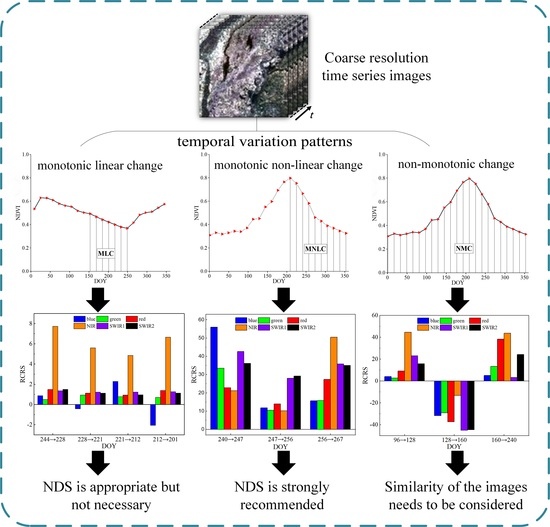
Figure 2 shows the averaged NDVI time series of BAH and NEA in 2016, extracted from Collection 6 MODIS NDVI products (MOD13A1 and MYD13A1). There are three kinds of temporal variation patterns in the time series of NDVI: monotonic linear change (MLC), monotonic nonlinear change (MNLC), and non-monotonic change (NMC). For the MLC, the NDVI shows monotonic and linear change during a period of time. An extreme situation of the MLC is that NDVI stays unchanging during a period of time (e.g., vegetation in the maturity period). For the MNLC, the NDVI shows monotonic and non-linear change during a period of time, which means the NDVI changes monotonically but is not stationary, and there are breaking points in the NDVI time series. For the NMC, the NDVI shows a non-monotonic change during a period of time, which means there is a turning point that exists in the NDVI time series. A NDVI time series shows non-monotonic changes when it covers both the vegetation growing phase and senescence phase.
For revealing the impact of input image dates on the accuracy of spatio-temporal fusion, time series of images containing temporal variation patterns of MLC, MNLC, and NMC are required. The NDVI time series of both BAH and NEA contains all three NDVI temporal variation patterns (as shown in Figure 3). Figure 4 shows the day of year (DOY) of HLS images (with more than 94% clear pixels) used in this study for both study areas.
3. Methodology
In this study, NDVI time series were extracted from the combined MOD13A1 and MYD13A1 for BAH and NEA areas, respectively. The input image pairs of HLS data at different dates were selected for MLC, MNLC, and NMLC periods, respectively. The ESTARFM fusion was conducted during MLC, MNLC, and NMLC periods, respectively, using input image pairs with different dates. The impacts of dates of input image pairs on the ESTARFM fusion accuracy were analyzed for MLC, MNLC, and NMLC periods, separately. The flowchart of the experiments and analysis is shown in Figure 5.
3.1. ESTARFM Algorithm
The enhanced STARFM (ESTARFM) was used as the spatio-temporal fusion algorithm for this study. The ESTARFM is a modified STARFM that employs a conversion coefficient to convert the reflectance changes of a mixed coarse resolution pixel to the fine resolution pixels within it [19]. By using at least two pairs of MODIS-HLS images acquired on the same date to participate in the fusion, the ESTARFM makes a more accurate prediction of reflectance in changing heterogeneous landscapes than STARFM does. For the ESTARFM, the HLS images of the predicted date tp is estimated by using the HLS image acquired on the date tn together with the corresponding MODIS images on these two dates according to Equation (1).
where H and M represent the HLS images and MODIS images, respectively, and their spatial resolutions are consistent. B is the predicted band, w is the length of the moving window (window size 51 × 51 in this study), and (xw/2, yw/2) is the position of the center pixel in the moving window; the value of the center pixel is what needs to be predicted in fusion. N is the total number of similar pixels in an extractable moving window, where similar pixels are defined as pixels that are similar to center pixels in reflectance. (xi, yi) is the location of each similar pixel, vi is the conversion coefficient of these similar pixels to adjust the temporal change from coarse pixels to fine pixels, and wi is the weight of the i-th similar pixel according to its contribution rate to the center pixel. For the ESTARFM algorithm, the spectral and distance weights were determined according to the spectral similarity and spatial distance between the similar pixels and the center pixel. The predicted HLS image Hm(xw/2, yw/2, tp, B) on the same date tp is obtained by using the HLS and MODIS images on another reference date tm according to Equation (1). To get a more accurate predicted HLS image on date tp, the two predicted HLS images (Hm(xw/2, yw/2, tp, B) and Hn(xw/2, yw/2, tp, B)) were added together considering the temporal weight as shown in Equation (2).
where, the H(xw/2, yw/2, tp, B) is the predicted HLS image on date tp. Tm and Tn are temporal weights of the two reference dates tm and tn. The sum of Tm and Tn is 1. The Tm and Tn are calculated by considering the similarity of images between the predicted date tp and the two reference dates tm and tn, respectively.
3.2. Selection of Input Image Pairs
The ESTARFM requires two input image pairs before and after the prediction date, separately. For convenience, we fixed the date of one input image pair and only changed the date of another input image pair. We named the prediction date as PD, the fixed date as FD, and the changing date as CD. In order to analyze the impacts of dates of input image pairs on the fusion accuracy, image pairs at CD need to be selected for different temporal variation patterns. Specifically, input image pairs at CDs for the MLC period, MNLC period, and NMC period were selected, respectively. In all cases, the image pairs at CD that were closer to the PD were selected successively, and the fusion accuracy of the input image pair at every CD was evaluated.
3.3. Accuracy Assessment
For each study area, the fused HLS-MODIS images were compared to the observed HLS images on PDs for fusion accuracy assessment. Only clear pixels were included for accuracy assessment. Since HLS adjusted the spectral bandpass of Sentinel-2 to Landsat-8, only Landsat-8 images in HLS are used as the true images for accuracy assessment. The metrics used for evaluation of the fusion accuracy are Coefficient of Determination (R2) and the Root Mean Square Error (RMSE). In order to analyze the changes of fusion accuracy as the CD of input image pairs are becoming closer to the PD, the Relative Change of R-Squared (RCRS) was defined to present the relative change rate of the R2 between the fused image with the input image at given CD, and the fused image with input image at another CD one more closer to PD. RCRS is calculated using Equation (3).
where R2 is the coefficient of determination of the fusion result with input image at a given CD, and is the coefficient of determination of the fusion result with input image at a CD one more closer to the PD. > 0 means the input image on date closer to PD leads to higher fusion accuracy. Conversely, < 0 means that input image on date closer to PD leads to lower fusion accuracy. = 0 indicates that the date of input images is independent to the fusion accuracy.
4. Results and Analysis
4.1. Impact of the CD on Fusion Accuracy for MLC Period
In BAH, HLS images at the PD (DOY is 196), the FD (DOY is 148), and the CDs (DOY are 201, 212, 221, 228, and 244, respectively) were selected for the ESTARFM fusion during the MLC period, as is shown in Figure 3a. The selected HLS data for the ESTARFM fusion experiments during the MLC period are listed in Table 1, in which S denotes the data are from Sentinel-2A and L denotes the data are from Landsat-8. The time interval denotes the date gap between the CD image and the PD image. The R2, RMSE, and RCRS of the fused results with input images at different CDs are shown in Figure 6. The standard false-color-composited images of the fused results and the true image at the PD are shown in Figure 7.
Figure 6 indicates that during the MLC period, for all bands, the fusion accuracies of the fused images increase when the CD of input images become closer to the PD, and the change of accuracy for different CDs is also monotonically linear. However, the improvement of fusion accuracies is insignificant. While the CDs changed from 244 to 201 (the time interval with PD changed from 48 to 5 days), except for the NIR band, the changes of R2 and RMSE are only about 0.05 and 0.01, separately, and the RCRS values of the most bands are less than 2%. For the NIR band, the R2 increased from 0.748 to 0.952, the RMSE decreased from 0.024 to 0.01, and the RCRS values are less than 8%. The results imply that for an MLC period, a closer input image date to the PD does not improve the fusion accuracy significantly. Figure 7 shows that the fused images with different CDs have no significant differences. This is because, for an MLC period, the effects of the linear differences among input images at different CDs could be partly compensated by the linear weights in the ESTARFM algorithm.
4.2. Impact of the CD on Fusion Accuracy for MNLC Period
To evaluate the impact of input image dates on ESTARFM fusion during the MNLC period of the NDVI time series (Figure 3b), the PD image (DOY is 272), the FD image (DOY is 336), and the CD images (DOY are 240, 247, 256, and 267) in the NEA were selected for analysis (Table 2). The R2, RMSE, and RCRS of the fused results at the PD with input images at different CDs are shown in Figure 8.
Figure 8 shows that as the CDs become closer to the PD, the fusion accuracies for the MNLC period increase nonlinearly (Figure 8a,b). This is different from the linear increase of the fusion accuracies for the MLC period (Figure 6a,b). When the time intervals between the CD and the PD changed from 32 to 5 days (the CDs changed from 240 to 267), the R2 nearly doubled for the MNLC period for all bands. In addition, the overall change of fusion accuracies for the MNLC (Figure 8a,b) are significantly higher than those for the MLC (Figure 6a,b). Specifically, for the NIR band (with the most significant change of accuracy in Section 4.1), when the time interval changed from 32 to 5 days, the R2 increased from 0.806 to 0.952 for the MLC (Section 4.1), and from 0.387 to 0.778 for the MNLC.
Overall, the RCRS values of all bands are over 10% for the MNLC period (Figure 8c), and for the MLC period, the RCRS values of the most bands are less than 2% and only the RCRS values of the NIR band only are near 8% (Figure 6c). We counted the overall situation of the RCRS values with the change of the CD for the MLC period and MNLC period, and the results are shown in Figure 9. The results show that with the change of the CD, the mean value of the RCSR for the MNLC (24.5485) is approximately fifteen times larger than the mean value of the RCSR for the MLC (1.6483).This is because for an MNLC period, the land surface reflectance changes monotonically but nonlinearly with the time, the similarity between the images at the CD and PD also shows nonlinear changes, so a linear weighting approach used in the ESTARFM is not sufficient to capture the nonlinear change.
The standard false-color-composited images of the fused images and the true image at the PD for the MNLC are shown in Figure 10. Unlike fused results for the MLC period (as shown in Figure 7), the results show the fused images with different CDs had significant differences. Specifically, the closer the CDs are to the PD, the more similar the fused images are to the true image in color.
These results indicate that for an MNLC period to achieve relatively high fusion accuracy, a much shorter time interval between the CD and PD is required than that for an MLC period. It implies that denser high spatial resolution observation is more effective for spatio-temporal fusion during the MNLC period than for the MLC period.
4.3. Impact of the CD on Fusion Accuracy for NMC Period
The image at the PD (the DOY is 272), the FD (the DOY is 336), and the CDs (add DOY of 96, 128, and 160 compared to Section 4.2) in the NEA were selected for the ESTARFM fusion experiments during the NMC period. The selected images are listed in Table 3. The NDVI value increases first and then decreases in the NEA area, as is shown in Figure 3c. The R2, RMSE, and RCRS of the fused results at the PD with different CDs are shown in Figure 11. The standard false-color-composited images of the fused results and the true image at the PD are shown in Figure 12.
As shown in Figure 11a,b, for the NMC, the fusion accuracies at the PD, based on input images at different CDs, change non-monotonically, which indicates that a closer input image date to the PD results in a lower fusion accuracy. Because the time series of the MNLC period is part of the time series of the NMC period (Figure 3b,c), the fusion accuracies at the PD (the DOY = 272) for the CDs at a DOY of 240, 247, 256, and 267, the fusion accuracies are exactly the same to those in Figure 8 (Figure 11). However, for the CDs at a DOY of 96, 128, and 160, which are before the date of the turning point (i.e., the DOY = 209) in the NDVI time series (Figure 3c), shorter time intervals between the CD and the PD do not lead to higher fusion accuracies. When the DOYs of the CD change from 128 to 160, the corresponding fusion accuracies are reduced (as shown in Figure 11a,b) and the RCRS values are negative (as shown in Figure 11c). This is because for the NMC period, when the CD and PD locate in the two sides of the turning point, the similarities between the images at the CD and the PD no longer depend on the time intervals between the CD and the PD. As shown in Figure 3c and Figure 12, the NDVI value and the standard false-color-composited image between DOY 128 and DOY 272 are more similar than those between DOY 160 and DOY 272. Thus, the fusion accuracies at DOY 272 based on the input image at DOY 128 are higher than those based on the input image at DOY 160. In particular, the standard false-color-composited image with the CD at DOY 128 for a sub-region are more similar in color to the true image than the one with the CD at DOY 160 (yellow boxes in Figure 12). Thus, for the spatio-temporal fusion during the NMC time period, the optimal selection of the input image date should not be based on the time interval between the CD and PD, but based on the similarity of the images at the CD and PD.
5. Discussions
This study investigated the impacts of different input image dates on the spatio-temporal fusion accuracy for a time series with different temporal variation patterns. The HLS 1.4 land surface reflectance was used as the fine spatial resolution data for its denser observation frequency, and MCD43A4 was used as the coarse spatial resolution data for spatio-temporal fusion. The most widely used spatio-temporal fusion algorithm, ESTARFM, was used for the investigation. The results of this paper revealed the impact of input image dates on the accuracy of spatio-temporal fusion for land surface with different temporal variations.
For the monotonic change (MC) period, inputting the image at a date closer to the prediction date (PD) largely leads to a higher fusion accuracy. In this case, the NDS is appropriate to the input image selection [23,25]. However, for the MLC and MNLC periods, the impact of the time interval between the input image date and the prediction date on the fusion accuracies varies. Given the same time interval between the input image date and the prediction date, the fusion accuracies for the temporal pattern of the MLC are much higher than those of the MNLC. This is because the linear change of the land surface reflectance in the MLC time series could be accurately modeled by the linear weight function used in the ESTARFM algorithm, but the nonlinear changes of the land surface reflectance in MNLC time series could not be captured well by a linear weight function. The results also show that for the MLC period, shorter intervals between the input image date and the prediction dates leads to a very small improvement (RCRS values of the most bands are less than 2% in this study) in fusion accuracy, which implies that the revisit period of a high spatial resolution image is less critical to the spatio-temporal fusion for land surface with MLC pattern. However, when the dates of the input image become closer to the PD, the increments of fusion accuracies for the MNLC period are much larger (more than 10 times) than those for the MLC period. Therefore, when the ESTARFM is applied to spatio-temporal fusion in the MNLC period, the input data with the date as close as possible to the PD, if there are any, is strongly recommended.
For the NMC period, the effect of the time interval between the input image date and the prediction date on the fusion accuracy is complex and cannot be characterized only by the time interval between the input image date and the prediction date. If the input image date and the prediction date are on the same side of the turning point in the NMC time series, in addition, the sub-sequence between the input and prediction dates is either MLC or MNLC, and the rules for MLC and MNLC hold true in this case. If the input image date and the prediction date are on the two sides of the turning point in the NMC time series, shorter time intervals between the input and prediction dates do not lead to a higher fusion accuracy. In such a case, the selection of the optimal input image date should not be dictated by the time interval but by the similarity between the input image and the image at the prediction date. The similarity between two dates is not only affected by the natural variation of the land surface, such as the growing and senescence of vegetation, but also by other factors such as land cover changes [24] and radiometric differences [26,28]. For the NMC time series, to select an optimal input image date for spatio-temporal fusion, the priori knowledge about the temporal variation pattern of the time series is necessary.
The findings of this paper provide important insights to the optimal selection of input image pairs based on the temporal variation patterns of land surface for spatio-temporal fusion. For the MC period, to get a fused image with a higher accuracy, inputted image pairs whose date is as close as possible to the PD are suggested. More specifically, for the MLC period, a longer time interval between the input image date and PD is acceptable if no input image is close to the PD available. This is particularly important in tropical areas where optimal images are to be contaminated by cloud cover. However, for the MNLC period, selecting the input image at the date closest to the PD is strongly recommended. In case no image at a date close to the PD is available from any single remote sensor, using harmonized multi-source high spatial resolution images such as those of the HLS is an effective solution to this problem. For the NMC period, the selection of the input image date should not be based on its closeness to the PD, whereas selecting the input image date based on the similarity between the input image date and the PD is a more reasonable choice. To get to know the similarity between two dates in the time series in advance, a coarse spatial resolution but with a high temporal resolution image time series from sensors such as MODIS and VIIRS are good references for learning the temporal variation pattern of land surface under study.
Strictly speaking, each band of each pixel in the image has its own temporal variation pattern. In theory, the optimal selection of the input image should be conducted pixel by pixel and band by band. Yet, this would make the selection of optimal input image much more complex and unpractical. For land surface, the reflectance changes over time are mainly caused by the land cover changes that could be approximately presented by the vegetation index. Therefore, from a practical perspective, the averaged NDVI time series is used to approximately represent the dominant temporal variations of land surface reflectance.
While this study focuses on the impact of input images on the spatio-temporal fusion accuracy, the effect of radiometric difference between the images taking part in the spatio-temporal fusion should be kept in mind [22,27,49], especially in cases that the harmonized multi-sensor remote sensing data, such as the HLS product, were used as the fine spatial resolution data for spatio-temporal fusion. In Figure 6c, when the DOY of input CD image changes from 228 to 221 and from 212 to 201, the RCRS values of the blue band are negative, which is unreasonable. The negative RCRS values of the blue band only occur when the input images from Landsat-8 to Sentinel-2A (the DOY of 228 vs. 212, and the DOY of 212 vs. 201 in Table 1) are compared. These negative RCRS values are probably caused by the inconsistency between the harmonized Landsat-8 OLI and Sentinel-2A MSI data in HLS 1.4. The less accurate harmonization of the blue band in HLS 1.4 had been reported by Claverie et al. [36] and Shang et al. [50].
6. Conclusions
Spatio-temporal fusion is an effective way to generate images with both high spatial and temporal resolutions. Previous studies have revealed that the accuracy of spatio-temporal fusion results partially depend on the input image pair used. However, the impacts of the different dates of the input image on the accuracy of spatio-temporal fusion for land surface with different temporal variation patterns have not been evaluated.
This study investigated the impacts of different dates for input images on the spatio-temporal fusion accuracy for time periods with the monotonic linear change (MLC), the monotonic nonlinear change (MNLC), and the non-monotonic change (NMC), respectively. The results revealed that:
- (1)
- The impacts of input image date on the accuracy of spatio-temporal fusion depend on the temporal variation patterns of the land surface between the input image date and the prediction date.
- (2)
- For time periods with a monotonic linear change (MLC), a shorter time interval between the input image date (CD) and the prediction date (PD) improves the fusion accuracy. The relationship between the degree of improvement in accuracy and the change of time intervals between the CD and the PD is also nearly linear. The differences of the fusion accuracies of different input image dates are not significant, which implies that a long time interval between the CD and the PD could yield high fusion accuracies for a time period with the MLC.
- (3)
- For time periods with a monotonic nonlinear change (MNLC), a shorter time interval between the input image date (CD) and the prediction date (PD) improves the fusion accuracy as well. The relationship between the degree of improvement in accuracy and the change of time intervals between the CD and the PD is non-linear. The impact of the interval between the CD and the PD on the fusion accuracy is more significant for the MNLC than for the MLC. Thus, for the MNLC, to obtain accurate fusion results, selecting an input image with a date close to the PD is strongly recommended.
- (4)
- For time periods with a non-monotonic change (NMC), in which there is a turning point between the input image date and the prediction date, the impacts of the input image date on the fusion accuracy are complex. A shorter time interval between the CD and the PD may lead to a lower fusion accuracy, whereas a longer time interval between the CD and the PD may lead to a higher fusion accuracy. For the NMC, the optimal selection of the input image date should not depend on the time interval, but on the similarity of the images between the CD and the PD.
The analysis of this paper is based on the ESTARFM. However, the conclusions we drew based on the ESTARFM are held for other weight function-based spatio-temporal fusion algorithms such as STARFM [6] and STAARCH [17]. Taking the temporal variation patterns accounted for in selecting the optimal input image date is also valuable for the hybrid spatio-temporal fusion algorithms such as FSDAM [25] and Fit-FC [51], and the learning-based spatio-temporal fusion algorithms [52,53,54].
Author Contributions
Conceptualization, A.S. and Y.B.; data processing and coding, A.S.; formal analysis, A.S., Y.B. and W.Z.; methodology, A.S. and Y.B.; funding acquisition, Y.B.; writing—original draft, A.S.; and writing—review and editing, A.S., Y.B. and Y.Z. All authors have read and agreed to the published version of the manuscript.
Funding
This study was jointly supported by the National Natural Science Foundation of China (Grant No. 41871232) and the National Key Research and Development Program of China (Grant No. 2016YFB0501502).
Data Availability Statement
All satellite remote sensing used in this study are openly and freely available. The Collection 6 MODIS product (MCD4344, MOD13A1, and MYD13A1) is available at https://search.earthdata.nasa.gov/search (accessed on 10 August 2021). The HLS data are freely accessible via https://hls.gsfc.nasa.gov/ (accessed on 6 July 2021).
Acknowledgments
This study was jointly supported by the National Natural Science Foundation of China (Grant No. 41871232) and the National Key Research and Development Program of China (Grant No. 2016YFB0501502). The authors also would like to acknowledge the NASA for providing the harmonized Landsat and Sentinel-2 (HLS) data product downloaded from https://hls.gsfc.nasa.gov/data/ (accessed on 6 July 2021) and the LP-DAAC and MODIS science team for providing free MODIS products. We also thank Xiaolin Zhu at the Hong Kong Poly-technic University for making the ESTARFM code available; Special thanks to Yaqian He at University of Central Arkansas and Yang Yang at Hydrology and Remote Sensing Laboratory, USDA for the English editing of the revised manuscript.
Conflicts of Interest
The authors declare no conflict of interest.
References
- Chen, J.M.; Chuvieco, E.; Wang, M. Preface, Special Issue of “50 Years of Environmental Remote Sensing Research: 1969–2019”. Remote Sens. Environ. 2021, 252, 112113. [Google Scholar] [CrossRef]
- Turner, W.; Rondinini, C.; Pettorelli, N.; Mora, B.; Leidner, A.K.; Szantoi, Z.; Buchanan, G.; Dech, S.; Dwyer, J.; Herold, M.; et al. Free and Open-Access Satellite Data Are Key to Biodiversity Conservation. Biol. Conserv. 2015, 182, 173–176. [Google Scholar] [CrossRef] [Green Version]
- Wulder, M.A.; Masek, J.G.; Cohen, W.B.; Loveland, T.R.; Woodcock, C.E. Opening the Archive: How Free Data Has Enabled the Science and Monitoring Promise of Landsat. Remote Sens. Environ. 2012, 122, 2–10. [Google Scholar] [CrossRef]
- Yang, B.; Liu, H.; Kang, E.L.; Shu, S.; Xu, M.; Wu, B.; Beck, R.A.; Hinkel, K.M.; Yu, B. Spatio-Temporal Cokriging Method for Assimilating and Downscaling Multi-Scale Remote Sensing Data. Remote Sens. Environ. 2021, 255, 112190. [Google Scholar] [CrossRef]
- Jia, D.; Cheng, C.; Song, C.; Shen, S.; Ning, L.; Zhang, T. A Hybrid Deep Learning-Based Spatiotemporal Fusion Method for Combining Satellite Images with Different Resolutions. Remote Sens. 2021, 13, 645. [Google Scholar] [CrossRef]
- Gao, F.; Masek, J.; Schwaller, M.; Hall, F. On the Blending of the Landsat and MODIS Surface Reflectance: Predicting Daily Landsat Surface Reflectance. IEEE Trans. Geosci. Remote Sens. 2006, 44, 2207–2218. [Google Scholar]
- Gómez, C.; White, J.C.; Wulder, M.A. Optical Remotely Sensed Time Series Data for Land Cover Classification: A Review. ISPRS J. Photogramm. Remote Sens. 2016, 116, 55–72. [Google Scholar] [CrossRef] [Green Version]
- Huang, C.; Goward, S.N.; Masek, J.G.; Thomas, N.; Zhu, Z.; Vogelmann, J.E. An Automated Approach for Reconstructing Recent Forest Disturbance History Using Dense Landsat Time Series Stacks. Remote Sens. Environ. 2010, 114, 183–198. [Google Scholar] [CrossRef]
- Lees, K.J.; Quaife, T.; Artz, R.R.E.; Khomik, M.; Clark, J.M. Potential for Using Remote Sensing to Estimate Carbon Fluxes across Northern Peatlands—A Review. Sci. Total Environ. 2018, 615, 857–874. [Google Scholar] [CrossRef]
- Tottrup, C.; Rasmussen, M.S. Mapping Long-Term Changes in Savannah Crop Productivity in Senegal through Trend Analysis of Time Series of Remote Sensing Data. Agric. Ecosyst. Environ. 2004, 103, 545–560. [Google Scholar] [CrossRef]
- Sun, L.; Gao, F.; Xie, D.; Anderson, M.; Chen, R.; Yang, Y.; Yang, Y.; Chen, Z. Reconstructing Daily 30 m NDVI over Complex Agricultural Landscapes Using a Crop Reference Curve Approach. Remote Sens. Environ. 2021, 253, 112156. [Google Scholar] [CrossRef]
- Li, X.; Zhou, Y.; Asrar, G.R.; Mao, J.; Li, X.; Li, W. Response of Vegetation Phenology to Urbanization in the Conterminous United States. Glob. Chang. Biol. 2017, 23, 2818–2830. [Google Scholar] [CrossRef] [PubMed]
- Liu, Q.; Fu, Y.H.; Zhu, Z.; Liu, Y.; Liu, Z.; Huang, M.; Janssens, I.A.; Piao, S. Delayed Autumn Phenology in the Northern Hemisphere Is Related to Change in Both Climate and Spring Phenology. Glob. Chang. Biol. 2016, 22, 3702–3711. [Google Scholar] [CrossRef] [PubMed]
- Chen, B.; Huang, B.; Xu, B. Comparison of Spatiotemporal Fusion Models: A Review. Remote Sens. 2015, 7, 1798–1835. [Google Scholar] [CrossRef] [Green Version]
- Wu, M.; Wu, C.; Huang, W.; Niu, Z.; Wang, C.; Li, W.; Hao, P. An Improved High Spatial and Temporal Data Fusion Approach for Combining Landsat and MODIS Data to Generate Daily Synthetic Landsat Imagery. Inf. Fusion 2016, 31, 14–25. [Google Scholar] [CrossRef]
- Zhu, X.; Cai, F.; Tian, J.; Williams, T.K.-A. Spatiotemporal Fusion of Multisource Remote Sensing Data: Literature Survey, Taxonomy, Principles, Applications, and Future Directions. Remote Sens. 2018, 10, 527. [Google Scholar] [CrossRef] [Green Version]
- Hilker, T.; Wulder, M.A.; Coops, N.C.; Linke, J.; McDermid, G.; Masek, J.G.; Gao, F.; White, J.C. A New Data Fusion Model for High Spatial- and Temporal-Resolution Mapping of Forest Disturbance Based on Landsat and MODIS. Remote Sens. Environ. 2009, 113, 1613–1627. [Google Scholar] [CrossRef]
- Roy, D.P.; Ju, J.; Lewis, P.; Schaaf, C.; Gao, F.; Hansen, M.; Lindquist, E. Multi-Temporal MODIS-Landsat Data Fusion for Relative Radiometric Normalization, Gap Filling, and Prediction of Landsat Data. Remote Sens. Environ. 2008, 112, 3112–3130. [Google Scholar] [CrossRef]
- Zhu, X.; Chen, J.; Gao, F.; Chen, X.; Masek, J.G. An Enhanced Spatial and Temporal Adaptive Reflectance Fusion Model for Complex Heterogeneous Regions. Remote Sens. Environ. 2010, 114, 2610–2623. [Google Scholar] [CrossRef]
- Liu, M.; Liu, X.; Dong, X.; Zhao, B.; Zou, X.; Wu, L.; Wei, H. An Improved Spatiotemporal Data Fusion Method Using Surface Heterogeneity Information Based on ESTARFM. Remote Sens. 2020, 12, 3673. [Google Scholar] [CrossRef]
- Knauer, K.; Gessner, U.; Fensholt, R.; Kuenzer, C. An ESTARFM Fusion Framework for the Generation of Large-Scale Time Series in Cloud-Prone and Heterogeneous Landscapes. Remote Sens. 2016, 8, 425. [Google Scholar] [CrossRef] [Green Version]
- Wang, P.; Gao, F.; Masek, J.G. Operational Data Fusion Framework for Building Frequent Landsat-Like Imagery. IEEE Trans. Geosci. Remote Sens. 2014, 52, 7353–7365. [Google Scholar] [CrossRef]
- Liu, M.; Yang, W.; Zhu, X.L.; Chen, J.; Chen, X.H.; Yang, L.Q.; Helmer, E.H. An Improved Flexible Spatiotemporal DAta Fusion (IFSDAF) method for producing high spatiotemporal resolution normalized difference vegetation index time series. Remote Sens. Environ. 2019, 227, 74–89. [Google Scholar] [CrossRef]
- Xie, D.; Gao, F.; Sun, L.; Anderson, M. Improving Spatial-Temporal Data Fusion by Choosing Optimal Input Image Pairs. Remote Sens. 2018, 10, 1142. [Google Scholar] [CrossRef] [Green Version]
- Zhu, X.L.; Helmer, E.H.; Gao, F.; Liu, D.S.; Chen, J.; Lefsky, M.A. A flexible spatiotemporal method for fusing satellite images with different resolutions. Remote Sens. Environ. 2016, 172, 165–177. [Google Scholar] [CrossRef]
- Walker, J.J.; De Beurs, K.M.; Wynne, R.H.; Gao, F. Evaluation of Landsat and MODIS data fusion products for analysis of dryland forest phenology. Remote Sens. Environ. 2012, 117, 381–393. [Google Scholar] [CrossRef]
- Gao, F.; Anderson, M.C.; Zhang, X.; Yang, Z.; Alfieri, J.G.; Kustas, W.P.; Mueller, R.; Johnson, D.M.; Prueger, J.H. Toward mapping crop progress at field scales through fusion of Landsat and MODIS imagery. Remote Sens. Environ. 2017, 188, 9–25. [Google Scholar] [CrossRef] [Green Version]
- Chen, Y.; Cao, R.Y.; Chen, J.; Zhu, X.L.; Zhou, J.; Wang, G.P.; Shen, M.G.; Chen, X.H.; Yang, W. A New Cross-Fusion Method to Automatically Determine the Optimal Input Image Pairs for NDVI Spatiotemporal Data Fusion. IEEE Trans. Geosci. Remote Sens. 2020, 58, 5179–5194. [Google Scholar] [CrossRef]
- Schreier, J.; Ghazaryan, G.; Dubovyk, O. Crop-Specific Phenomapping by Fusing Landsat and Sentinel Data with MODIS Time Series. Eur. J. Remote Sens. 2021, 54, 47–58. [Google Scholar] [CrossRef]
- Cooley, S.W.; Smith, L.C.; Stepan, L.; Mascaro, J. Tracking Dynamic Northern Surface Water Changes with High-Frequency Planet CubeSat Imagery. Remote Sens. 2017, 9, 1306. [Google Scholar] [CrossRef] [Green Version]
- Gao, F.; Hilker, T.; Zhu, X.; Anderson, M.; Masek, J.; Wang, P.; Yang, Y. Fusing Landsat and MODIS Data for Vegetation Monitoring. IEEE Geosci. Remote Sens. Mag. 2015, 3, 47–60. [Google Scholar] [CrossRef]
- Wang, Q.; Blackburn, G.A.; Onojeghuo, A.O.; Dash, J.; Zhou, L.; Zhang, Y.; Atkinson, P.M. Fusion of Landsat 8 OLI and Sentinel-2 MSI Data. IEEE Trans. Geosci. Remote Sens. 2017, 55, 3885–3899. [Google Scholar] [CrossRef] [Green Version]
- Liu, Y.; Zuo, X.; Tian, J.; Li, S.; Cai, K.; Zhang, W. Research on Generic Optical Remote Sensing Products: A Review of Scientific Exploration, Technology Research, and Engineering Application. IEEE J. Sel. Top. Appl. Earth Obs. Remote Sens. 2021, 14, 3937–3953. [Google Scholar] [CrossRef]
- Zhu, Z.; Wang, S.; Woodcock, C.E. Improvement and Expansion of the Fmask Algorithm: Cloud, Cloud Shadow, and Snow Detection for Landsats 4–7, 8, and Sentinel 2 Images. Remote Sens. Environ. 2015, 159, 269–277. [Google Scholar] [CrossRef]
- Zhang, H.K.; Roy, D.P.; Yan, L.; Li, Z.; Huang, H.; Vermote, E.; Skakun, S.; Roger, J.C. Characterization of Sentinel-2A and Landsat-8 Top of Atmosphere, Surface, and Nadir BRDF Adjusted Reflectance and NDVI Differences. Remote Sens. Environ. 2018, 215, 482–494. [Google Scholar] [CrossRef]
- Vermote, E.; Justice, C.; Claverie, M.; Franch, B. Preliminary Analysis of the Performance of the Landsat 8/OLI Land Surface Reflectance Product. Remote Sens. Environ. 2016, 185, 46–56. [Google Scholar] [CrossRef]
- Masek, J.G.; Vermote, E.F.; Saleous, N.E.; Wolfe, R.; Hall, F.G.; Huemmrich, K.F.; Gao, F.; Kutler, J.; Lim, T.K. A Landsat Surface Reflectance Dataset for North America, 1990–2000. IEEE Geosci. Remote Sens. Lett. 2006, 3, 68–72. [Google Scholar] [CrossRef]
- Doxani, G.; Vermote, E.; Roger, J.C.; Gascon, F.; Adriaensen, S.; Frantz, D.; Hagolle, O.; Hollstein, A.; Kirches, G.; Li, F.; et al. Atmospheric Correction Inter-Comparison Exercise. Remote Sens. 2018, 10, 352. [Google Scholar] [CrossRef] [Green Version]
- Foga, S.; Scaramuzza, P.L.; Guo, S.; Zhu, Z.; Dilley, R.D.; Beckmann, T.; Schmidt, G.L.; Dwyer, J.L.; Joseph Hughes, M.; Laue, B. Cloud Detection Algorithm Comparison and Validation for Operational Landsat Data Products. Remote Sens. Environ. 2017, 194, 379–390. [Google Scholar] [CrossRef] [Green Version]
- Masek, J. Automated Registration and Orthorectification Package for Landsat and Landsat-like Data Processing. J. Appl. Remote Sens. 2009, 3, 033515. [Google Scholar] [CrossRef]
- Roy, D.P.; Zhang, H.K.; Ju, J.; Gomez-Dans, J.L.; Lewis, P.E.; Schaaf, C.B.; Sun, Q.; Li, J.; Huang, H.; Kovalskyy, V. A General Method to Normalize Landsat Reflectance Data to Nadir BRDF Adjusted Reflectance. Remote Sens. Environ. 2016, 176, 255–271. [Google Scholar] [CrossRef] [Green Version]
- Roy, D.P.; Li, J.; Zhang, H.K.; Yan, L.; Huang, H.; Li, Z. Examination of Sentinel-2A Multi-Spectral Instrument (MSI) Reflectance Anisotropy and the Suitability of a General Method to Normalize MSI Reflectance to Nadir BRDF Adjusted Reflectance. Remote Sens. Environ. 2017, 199, 25–38. [Google Scholar] [CrossRef]
- Claverie, M.; Ju, J.; Masek, J.G.; Dungan, J.L.; Vermote, E.F.; Roger, J.C.; Skakun, S.V.; Justice, C. The Harmonized Landsat and Sentinel-2 Surface Reflectance Data Set. Remote Sens. Environ. 2018, 219, 145–161. [Google Scholar] [CrossRef]
- Pastick, N.J.; Wylie, B.K.; Wu, Z. Spatiotemporal Analysis of Landsat-8 and Sentinel-2 Data to Support Monitoring of Dryland Ecosystems. Remote Sens. 2018, 10, 791. [Google Scholar] [CrossRef] [Green Version]
- Torbick, N.; Huang, X.; Ziniti, B.; Johnson, D.; Masek, J.; Reba, M. Fusion of Moderate Resolution Earth Observations for Operational Crop Type Mapping. Remote Sens. 2018, 10, 1058. [Google Scholar] [CrossRef] [Green Version]
- Schaaf, C.B.; Gao, F.; Strahler, A.H.; Lucht, W.; Li, X.; Tsang, T.; Strugnell, N.C.; Zhang, X.; Jin, Y.; Muller, J.; et al. First Operational BRDF, Albedo Nadir Reflectance Products from MODIS. Remote Sens. Environ. 2002, 83, 135–148. [Google Scholar] [CrossRef] [Green Version]
- Wang, Z.; Schaaf, C.B.; Strahler, A.H.; Chopping, M.J.; Román, M.O.; Shuai, Y.; Woodcock, C.E.; Hollinger, D.Y.; Fitzjarrald, D.R. Evaluation of MODIS Albedo Product (MCD43A) over Grassland, Agriculture and Forest Surface Types during Dormant and Snow-Covered Periods. Remote Sens. Environ. 2014, 140, 60–77. [Google Scholar] [CrossRef] [Green Version]
- Wang, Z.; Schaaf, C.B.; Sun, Q.; Shuai, Y.; Román, M.O. Capturing Rapid Land Surface Dynamics with Collection V006 MODIS BRDF/NBAR/Albedo (MCD43) Products. Remote Sens. Environ. 2018, 207, 50–64. [Google Scholar] [CrossRef]
- Gao, F.; He, T.; Masek, J.G.; Shuai, Y.; Schaaf, C.; Wang, Z. Angular Effects and Correction for Medium Resolution Sensors to Support Crop Monitoring. IEEE J. Sel. Top. Appl. Earth Obs. Remote Sens. 2014, 7, 4480–4489. [Google Scholar]
- Shang, R.; Zhu, Z. Harmonizing Landsat 8 and Sentinel-2: A time-series-based reflectance adjustment approach. Remote Sens. Environ. 2019, 235, 111439. [Google Scholar] [CrossRef]
- Wang, Q.; Atkinson, P.M. Spatio-temporal fusion for daily Sentinel-2 images. Remote Sens. Environ. 2018, 204, 31–42. [Google Scholar] [CrossRef] [Green Version]
- Wang, X.; Wang, X. Spatiotemporal Fusion of Remote Sensing Image Based on Deep Learning. J. Sens. 2020, 2020, 8873079. [Google Scholar] [CrossRef]
- Li, W.; Zhang, X.; Peng, Y.; Dong, M. Spatiotemporal Fusion of Remote Sensing Images Using a Convolutional Neural Network with Attention and Multiscale Mechanisms. Int. J. Remote Sens. 2021, 42, 1973–1993. [Google Scholar] [CrossRef]
- Jia, D.; Song, C.; Cheng, C.; Shen, S.; Ning, L.; Hui, C. A Novel Deep Learning-Based Spatiotemporal Fusion Method for Combining Satellite Images with Different Resolutions Using a Two-Stream Convolutional Neural Network. Remote Sens. 2020, 12, 698. [Google Scholar] [CrossRef] [Green Version]
Figure 1.
Standard false-color-composite images of NEA area and BAH area on 11 May 2016 and 28 September 2016, respectively.
Figure 1.
Standard false-color-composite images of NEA area and BAH area on 11 May 2016 and 28 September 2016, respectively.

Figure 2.
Time series of NDVI for study area (a) BAH and (b) NEA.

Figure 3.
Temporal variation in the three sets of NDVI (Pointed out by vertical line). (a) MLC, (b) MNLC, and (c) NMC.
Figure 3.
Temporal variation in the three sets of NDVI (Pointed out by vertical line). (a) MLC, (b) MNLC, and (c) NMC.

Figure 4.
DOY of HLS images used in (a) BAH area and (b) NEA area.

Figure 5.
Flowchart of method.

Figure 6.
Accuracies of the fused images with different CDs for the MLC period. (a) R2, (b) RMSE, and (c) RCRS (The horizontal axis indicates the DOY of the input CD image pairs for (a,b), and the change of DOY for (c); the vertical axis indicates the values of R2, RMSE, and RCRS, respectively).
Figure 6.
Accuracies of the fused images with different CDs for the MLC period. (a) R2, (b) RMSE, and (c) RCRS (The horizontal axis indicates the DOY of the input CD image pairs for (a,b), and the change of DOY for (c); the vertical axis indicates the values of R2, RMSE, and RCRS, respectively).

Figure 7.
Standard false-color-composite images of the fused images with different CDs for the MLC period and the true image.
Figure 7.
Standard false-color-composite images of the fused images with different CDs for the MLC period and the true image.

Figure 8.
Accuracies of the fused images with different CDs for the MNLC period. (a) R2, (b) RMSE, and (c) RCRS (the horizontal axis indicates the DOY of the input CD image pairs for (a,b), and the change of DOY for (c); the vertical axis indicates the values of R2, RMSE, and RCRS, respectively).
Figure 8.
Accuracies of the fused images with different CDs for the MNLC period. (a) R2, (b) RMSE, and (c) RCRS (the horizontal axis indicates the DOY of the input CD image pairs for (a,b), and the change of DOY for (c); the vertical axis indicates the values of R2, RMSE, and RCRS, respectively).

Figure 9.
Boxplots of RCRS with CD for (a) MLC period and (b) MNLC period. The red number represents average value, and the black number is the upper quartile, the median, and the lower quartile from top to bottom.
Figure 9.
Boxplots of RCRS with CD for (a) MLC period and (b) MNLC period. The red number represents average value, and the black number is the upper quartile, the median, and the lower quartile from top to bottom.

Figure 10.
Standard false-color-composited images of the fused images with different CDs for the MNLC period and the true image.
Figure 10.
Standard false-color-composited images of the fused images with different CDs for the MNLC period and the true image.

Figure 11.
Accuracies of the fused images with different CDs for NMC period. (a) R2, (b) RMSE, and (c) RCRS (The horizontal axis indicates the DOY of the input CD image pairs for (a,b), and the change of DOY for (c); the vertical axis indicates the values of R2, RMSE, and RCRS, respectively).
Figure 11.
Accuracies of the fused images with different CDs for NMC period. (a) R2, (b) RMSE, and (c) RCRS (The horizontal axis indicates the DOY of the input CD image pairs for (a,b), and the change of DOY for (c); the vertical axis indicates the values of R2, RMSE, and RCRS, respectively).

Figure 12.
Standard false-color-composited images of the fused results with different input image dates for the NMC period and the true image (yellow box highlights a sub-region).
Figure 12.
Standard false-color-composited images of the fused results with different input image dates for the NMC period and the true image (yellow box highlights a sub-region).


Table 1.
Data selected for MLC period.
| FD (DOY) | PD (DOY) | CD (DOY) | Time Interval (Days) |
|---|---|---|---|
| 148 | 196 | 244 (L) | 48 |
| 148 | 196 | 228 (L) | 32 |
| 148 | 196 | 221 (S) | 25 |
| 148 | 196 | 212 (L) | 16 |
| 148 | 196 | 201 (S) | 5 |
Table 2.
Data selected for MNLC period.
| CD (DOY) | PD (DOY) | FD (DOY) | Time Interval (Days) |
|---|---|---|---|
| 240 (L) | 272 | 336 | 32 |
| 247 (S) | 272 | 336 | 25 |
| 256 (L) | 272 | 336 | 16 |
| 267 (S) | 272 | 336 | 5 |
Table 3.
Data selected for NMC period.
| CD (DOY) | PD (DOY) | FD (DOY) | Time Interval (Days) |
|---|---|---|---|
| 96 (L) | 272 | 336 | 176 |
| 128 (L) | 272 | 336 | 144 |
| 160 (L) | 272 | 336 | 112 |
| 240 (L) | 272 | 336 | 32 |
| 247 (S) | 272 | 336 | 25 |
| 256 (L) | 272 | 336 | 16 |
| 267 (S) | 272 | 336 | 5 |
Publisher’s Note: MDPI stays neutral with regard to jurisdictional claims in published maps and institutional affiliations. |
© 2022 by the authors. Licensee MDPI, Basel, Switzerland. This article is an open access article distributed under the terms and conditions of the Creative Commons Attribution (CC BY) license (https://creativecommons.org/licenses/by/4.0/).
Share and Cite
MDPI and ACS Style
Shen, A.; Bo, Y.; Zhao, W.; Zhang, Y. Impact of the Dates of Input Image Pairs on Spatio-Temporal Fusion for Time Series with Different Temporal Variation Patterns. Remote Sens. 2022, 14, 2431. https://doi.org/10.3390/rs14102431
AMA Style
Shen A, Bo Y, Zhao W, Zhang Y. Impact of the Dates of Input Image Pairs on Spatio-Temporal Fusion for Time Series with Different Temporal Variation Patterns. Remote Sensing. 2022; 14(10):2431. https://doi.org/10.3390/rs14102431
Chicago/Turabian StyleShen, Aojie, Yanchen Bo, Wenzhi Zhao, and Yusha Zhang. 2022. "Impact of the Dates of Input Image Pairs on Spatio-Temporal Fusion for Time Series with Different Temporal Variation Patterns" Remote Sensing 14, no. 10: 2431. https://doi.org/10.3390/rs14102431
Note that from the first issue of 2016, this journal uses article numbers instead of page numbers. See further details here.