
Adaptive Polar-Grid Gaussian-Mixture Model for Foreground Segmentation Using Roadside LiDAR


Department of Instrument Science and Technology, School of Automation and Electrical Engineering, University of Science and Technology Beijing, Beijing 100083, China
*
Author to whom correspondence should be addressed.
†
These authors contributed equally to this work.
Remote Sens. 2022, 14(11), 2522; https://doi.org/10.3390/rs14112522
Submission received: 15 April 2022
/
Revised: 21 May 2022
/
Accepted: 23 May 2022
/
Published: 25 May 2022
(This article belongs to the Special Issue Laser Scanning and Point Cloud Processing in Urban Environments)
Abstract
:Roadside LiDAR has become an important sensor for the detection of objects in cities, such as vehicles and pedestrians, which is due to its advantages of all-weather operation and high-ranging accuracy. In order to serve an intelligent transportation system, the efficient and accurate segmentation of vehicles and pedestrians is needed in the coverage area of the LiDAR. In this study, a roadside LiDAR was fixed on brackets on both sides of the road to obtain the point-cloud information on the urban road and the surrounding environment. A segmentation method that is based on a scanning LiDAR sensor is proposed. First, a polar grid that is based on polar coordinates is constructed to count the LiDAR rotations to obtain the original information of the angle and the distance of the point cloud, and the background point-cloud image is dynamically updated over time. By aiming at the complex urban road environment and the interference of trees and light poles in the background, an adaptive polar-grid Gaussian-mixture model (APG-GMM) that uses a point-cloud method is proposed to improve the accuracy of the foreground and background segmentation. A density-adaptive DBSCAN target-clustering algorithm is proposed, as well as a dynamic adaptive neighborhood radius, to solve the problem of the low clustering accuracy that is caused by the uneven density of point clouds that are collected by LiDAR, and to divide the point clouds in the foreground into vehicles and pedestrians. Finally, the method was tested at intersections and urban roads with dense traffic flows. The experimental results show that the proposed algorithm can segment the foreground and background well and can cluster vehicles and pedestrians while reducing the number of calculations and the time complexity.
1. Introduction
In recent years, intelligent transportation systems [1,2] have achieved good results in improving the safety [3] and efficiency of urban traffic and in reducing urban congestion [4]. The current mainstream sensors that are used in environmental perception in intelligent transportation systems are image sensors [5] and the light detection and ranging (LiDAR) sensor [6]. Image sensors have high pixel resolutions and high frame rates, and the urban-road-traffic video that is collected by image sensors can obtain rich target information, such as shape-feature, color-feature, and texture-feature information, for environment perception. However, the image sensor is a passive sensor that requires ambient lighting for imaging, and the intensity of the image changes with illumination [7]. This makes it difficult to image at night and leads to poor quality because of the production of more noise in the image. It becomes difficult to obtain vehicle and pedestrian information on the urban road since the image sensor is easily disturbed by outside light. In addition, it is difficult to obtain the precise distance information of the target with an image sensor. LiDAR is an active sensor that emits laser beams and receives echo laser beams to measure the distance and the reflection intensity of its target. Compared to image sensors, the LiDAR sensor emits laser beams actively and receives the reflected laser beams. Therefore, LiDAR achieves good imaging results during the day and night, and it does not require an external light source. It can collect the precise distance information of a target through time-of-flight (ToF) or frequency-modulated continuous-wave (FMCW) ranging methods in order to obtain 3D information on the target and the surrounding environment. Because of its advantages of high-ranging accuracy and the fact that it is not affected by external ambient light, LiDAR has gradually become an essential sensor for environmental perception in urban intelligent transportation systems.
With the reduction in the cost of LiDAR, it is possible to deploy roadside LiDAR on urban roads. Roadside LiDAR is arranged at high heights, such as on traffic poles or streetlights, which means that the vehicles are less occluded from each other, and the measurement range is 100 m. When using roadside LiDAR to extract traffic-target information, the LiDAR point-cloud data contain traffic-target information and background information. However, roadside LiDAR datasets are extremely large, and the surrounding environments of urban and suburban roads are complex when the traffic flow is heavy. The background information of urban roads is complex, and it includes roads, traffic facilities, surrounding buildings, trees on the roadside, etc. This poses a challenge for roadside LiDAR in the accurate and efficient identification of vehicles and pedestrians on roads with complex background environments. The premise of vehicle-target recognition and location is to accurately segment the vehicle target [8,9]. In order to extract objects from the point-cloud data that are collected by roadside LiDAR, various object-segmentation methods have been developed. The methods of point-cloud segmentation that are based on point features include edge-based segmentation [10], region-based segmentation [11,12,13], model-based segmentation [14,15,16], and machine-learning segmentation [17,18,19]. These methods have high computational complexity and slow running speeds. With the development of deep neural networks, more and more methods that use deep neural networks have been springing up to realize point-cloud segmentation [20,21,22]. These methods require a large amount of data for the model training.
Background filtering is one of the methods of moving-object segmentation that preserves the foreground data by filtering out the background data in the original data. It is commonly used in smart video surveillance [23], traffic surveillance and analysis [24], human detection [25] and tracking, and automatic sports-video [26] analysis. Although background filtering has been widely used in the processing of 2D images, it is still difficult to perform on irregular and disordered 3D point clouds directly [27]. In the process of roadside LiDAR point-cloud detection, background filtering [28] is an important step to reduce the complexity of the data processing, and it is the first step for target detection and tracking [9].
The roadside LiDAR sensor collects 360° data. However, we are only interested in the foreground as the vehicles and pedestrians on the road. The point cloud of vehicles and pedestrians only occupies a small part of the point cloud in a frame, and a large number of point clouds are in the background. This includes surrounding buildings, trees, the ground, and fixed transportation facilities. The greater the number of point clouds, the higher the computing power that is required for target detection. Filtering a large number of backgrounds can save computing power and energy consumption, reduce the processing time, and improve the roadside response speed to vehicle identification. To segment the foreground by using roadside LiDAR, different background-filtering methods have been proposed in recent years. The most traditional background-filtering method is to select frames without the foreground as background frames manually [29]. However, on urban roads, it is difficult to find frames without the foreground in urban traffic. Therefore, subspace cubes and cube-based [30] background-filtering methods have been proposed to segment the background in traffic flow. Statistical and geometric methods are used to select frames without the foreground in the subspace, and to combine these subspaces to form background frames. However, it becomes difficult to choose the appropriate grid size to create the background model in the case of heavy traffic [30]. When the background changes, the background frame needs to be refreshed. Moreover, the environment is complicated, and the background, such as swaying leaves on the roadside, can easily be mistaken for the foreground. To solve the problems of accurately determining the background position in the complex urban road environment and of improving the segmentation accuracy of the background, we focused on building the adaptive polar-grid Gaussian-mixture model, which is based on the polar grid, by using roadside LiDAR. The main contributions of our proposed method can be summarized as follows:
1. We propose a new method that uses spherical coordinates to build grids for roadside LiDAR, which are named polar grids. According to the angular resolution of LiDAR, an environment-background spherical-coordinate grid is established and automatically generated. The polar grid uses spherical coordinates to ensure that the density of the point cloud of every grid is the same at different distances. Compared with the cube-based grid method, the polar grid is not affected by distance;
2. A new adaptive polar-grid Gaussian-mixture model is proposed. By establishing multiple Gaussian models on the basis of a polar grid, the problems of accurately determining the background position in the complex urban road environment and of improving the segmentation accuracy of the background are solved. The point cloud that is collected by the LiDAR is divided into two categories: background and foreground;
3. A density-adaptive DBSCAN target-clustering algorithm is proposed, and a dynamic adaptive neighborhood radius is proposed to solve the problem of the low clustering accuracy that is caused by the uneven density of the point clouds collected by LiDAR. In this way, the accurate segmentation of vehicles and pedestrians is achieved.
The rest of this paper is organized as follows. The second part introduces the method that we propose in detail. The third part presents the LiDAR data acquisition. The experimental results and analysis are shown in the fourth part. A discussion about the experimental results is shown in the fifth part. Finally, the sixth part summarizes the paper and gives the conclusions.
2. Materials and Methods
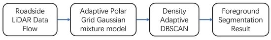
In this section, we elaborate on the segmentation method for roadside LiDAR vehicles on urban roads. We introduce the principle and characteristics of rotating LiDAR first, and then the polar-grid mask and the adaptive polar-grid Gaussian-mixture model is proposed. Finally, a density-adaptive DBSCAN target-clustering method is proposed. Figure 1 shows the schematic block diagram of the proposed method. The three parts of the diagram are the input, the model, and the segmentation. The input of our proposed method is the point-cloud data flow collected by the LiDAR, and the polar grid that is established by the APG-GMM is used to divide the point cloud into foreground and background. Finally, the foreground, such as vehicles, is segmented through density-adaptive DBSCAN.
2.1. Background-Separation Theory Based on Rotation LiDAR
LiDAR is an active sensor that targets an object with laser beams and measures the time for the reflected light to return to the receiver to calculate the precise distance of objects, as is shown in Figure 2. Mechanical-rotation LiDAR installs the laser-emitting unit and the receiving unit on a vertical axis, and it rotates along the vertical axis to collect point-cloud data. Figure 3 shows the schematic diagram of mechanical rotating LiDAR. Laser beams are emitted in a specific order, and they are received by the receiving unit after being reflected by objects or backgrounds. A laser-emitting unit and a receiving unit form a detector module. For LiDAR, 16, 32, 64, or more detector modules are actually installed. Each of the detector modules is represented by a laser ID, and the vertical angle of every module is calibrated in the factory. The detector rotates around the Z axis during the period of rotation (γ) under the control of a motor.
The working principle of the LiDAR sensor is as follows: The laser that is emitted by the semiconductor laser unit is beam-shaped in a detector module and is emitted from the LiDAR window. Part of the laser returns to the LiDAR with the same optical path and is received by the detector module after being reflected on the surface of the object. The LiDAR converts the light signal into electrical signals to calculate the position of the target. The position information of every point includes the laser ID, azimuth, distance, intensity, and timestamp through the processing of the signal by the LiDAR. The motor of the LiDAR sensor rotates 360° to scan the surrounding environment once to form the frame of a LiDAR point cloud.
A ToF ranging method is used to calculate the distance between the LiDAR and the point of the object (). That is, the distance () between the LiDAR and the point () can be calculated as:
where denotes the speed of light, and denotes the time from laser emission to reception. When the LiDAR rotates, a point () can be expressed in a spherical-coordinate system as:
where represents the vertical angle of the corresponding laser-ID detector module.
The motor drives the detector module of the LiDAR to rotate, and so the point clouds of each frame cannot overlap. Moreover, the detector module cannot receive the echo laser when the reflectivity is lower than 10%, which means that the distance exceeds the detection range of the LiDAR. In some cases, the LiDAR cannot return the distance information for all angles, and so the number of point clouds that is returned in each frame is different. Therefore, the point cloud that is collected by LiDAR is not voxel grid data, and it is different from the image.
In addition, roadside LiDAR is usually mounted on traffic poles or roadside tripods. Compared to vehicle LiDAR, the higher installation height reduces the occlusion of the vehicle and is conducive to receiving more information. Figure 4 shows the point cloud collected by the LiDAR at different heights. The higher the erection height, the wider the perception range of the LiDAR, and the more road and vehicle information can be obtained. Vehicle LiDAR is generally installed at the front of the car. The limited installation height of the vehicle LiDAR and vehicle occlusion result in a large blind spot. Since roadside LiDAR is installed on traffic poles at the roadside, the installation height is higher than that of vehicle LiDAR, which makes the field of view wider and reduces the blind spot that is caused by vehicle occlusion.
As is shown in Figure 5, roadside LiDAR data were collected at a bustling intersection for 20 min, and 1000 frames of data were chosen to count the number of foreground and background point clouds. The proportion of foreground point clouds to the total number of point clouds is less than 33%, and the mean ratio of the foreground point is 12.79% in the 1000 frames at bustling urban intersections. It can be seen that filtering the background points from the point cloud can greatly reduce the computational cost of the segmentation of the foreground points, such as vehicles and pedestrians.
2.2. Polar Grid of Background
On the roadside, the environment of the LiDAR sensor is more complicated, and features of the background, such as swaying leaves on the roadside, can easily be mistaken for the foreground. Xu H [31] established multiple subspace cubes in the point-cloud data flow and composed a background map by selecting subspace cubes without vehicles. Wang G [32] proposed a cube-based background-filtering method that uses multiple point-cloud frames to establish a statistical background model to select background frames. A 3D density-statistic-filtering (3D-DSF) [8,33] method was proposed that uses segmented cubes to solve the background-extraction problem. These methods of background-frame establishment all use cube-based grids [34]. However, it becomes difficult to choose the appropriate grid size to create the background model in the case of heavy traffic [30]. Therefore, we propose a polar-grid-based model to segment the background and foreground, which can help us to segment the foreground and background during heavy traffic by using rotating LiDAR.
According to the characteristics of rotating LiDAR, the polar background grid is established with the azimuth and vertical angle so that the points in each frame can be placed in the azimuth and vertical-angle grid. The polar background grid () is:
where is the parameter of each polar grid, and represents the number of vertical-angle grids. This is determined by the number of LiDAR detector modules. represents the number of horizontal-angle grids. The horizontal angle (l) of each polar grid is:
This divides the range of the LiDAR detection into a conical space of . Although the azimuth of the point from the same detector module is different after a period, every point falls into a polar grid with the roadside LiDAR in the center, as is shown in Figure 6.
Because of the characteristics of LiDAR rotational scanning, the rectangular-grid method has a high density of point clouds at close ranges and sparse point clouds at long ranges. The polar grid that is proposed can ensure the same point-cloud density for each grid, which allows us to better model the background.
2.3. Proposed Model: APG-GMM
The traditional Gaussian-mixture model [35,36,37] is used for image background modeling. In our proposed APG-GMM model, each polar grid is an independent random variable. Therefore, a Gaussian model is established independently for each polar grid. These Gaussian distributions can describe the background information. For urban roads, there are various background objects in the polar grid, such as trees, pole-like traffic facilities, and background walls. Therefore, multiple Gaussian distributions are needed to describe the background information in the polar grid. As is shown in Figure 7, there are two background objects, including a tree and a wall, in the polar grid. Echo signals of different background objects are obtained from laser beams in different frames. When the background environment of a polar grid is complex and it involves objects such as trees or pole-like traffic facilities, multiple Gaussian distributions are required to describe the real background situation. On the contrary, only a Gaussian distribution with the highest priority is needed to accurately describe the background when the background environment is simple. When the background changes, we implement the dynamic updating of the background point cloud by updating multiple Gaussian-distribution parameters.
For point in a point-cloud data flow, suppose its distance value at time () is . Gaussian distributions are used to describe these distance values, and the probability density function of is represented by the weighted mixture of Gaussian distributions as follows:
In the formula, , , and are the weight, mean, and covariance matrix of the Gaussian distribution of the Gaussian-mixture model at time (), and the sum of weights is 1. is the probability density function of the Gaussian distribution, which is given by:
According to the above analysis, the algorithm of the APG-GMM in the paper is described below:
Step (1) Initialize the model. Read the first frame of the LiDAR data and input the distance value () of each point as into the corresponding polar grid (). If a polar grid has more than one point, the maximum distance of all points is used as the value () of the polar grid;
Step (2) Set a larger covariance () and a smaller weight () as initial parameters;
Step (3) Update the model parameters. At the frame, we compare with the average of Gaussian distributions, respectively, and select the matching Gaussian distribution according to the following formula:
where is a coefficient. If the relationship between the value of a point and the Gaussian distribution satisfies the above formula, it means that the point matches the Gaussian distribution. The matched Gaussian-distribution parameters are updated according to the following formula:
where is the parameter learning rate, is the custom learning rate, and . The weights of Gaussian distributions are updated as follows:
Step (4) Dynamic updating. The dynamic updating of the background point cloud is accomplished by updating the parameters of the Gaussian distributions on the basis of the polar grid. If the current grid does not match the Gaussian distribution, the mean and variance parameters of the grid deviate greatly from the real background value, and so a new Gaussian distribution is constructed to replace the distribution with the smallest priority. Additionally, the constructed Gaussian distribution uses the parameters that are set in the initialization background and uses the current frame value () as the mean. After the update is completed, the weight of each Gaussian distribution is normalized to maintain the sum of the weights as 1. In order to improve the credibility of the background model, the weights are normalized as follows:
When the parameters of the model of some grids in the polar grid are similar, some Gaussian distributions can be combined. After the model parameters are updated, if the difference between the means of the two Gaussian distributions (m and n) of the same grid is less than the threshold (), the two Gaussian distributions are combined into one. This step can combine similar Gaussian distributions and reduce model redundancy. At the same time, it has better adaptability to sparse swaying trees. The updated method is as follows:
Step (6) Polar grid of background extraction. For each polar grid of the Gaussian distribution, sort the distributions in descending order according to the ratio: . The Gaussian distribution belonging to the background map is judged as follows:
where is the threshold. The polar grid of the background consists of Gaussian models. Foreground segmentation involves background filtering by comparing the point cloud of the current frame to the background model to separate the foreground and background. If the current point does not belong to any one of the Gaussian distributions, the point is a foreground point. This background-segmentation method can be expressed as follows:
where is a certain point, a value of 1 represents a foreground point, and a value of 0 represents a background point.
2.4. Proposed Algorithm: Density-Adaptive DBSCAN for Target Clustering
Density-based spatial clustering of applications with noise (DBSCAN) [38,39] is a density-clustering algorithm that was proposed by Ester et al. This method is applied to the point-cloud clustering of any complex shape, and it does not require a given number of clusters [40]. The parameters of the algorithm are the neighborhood radius () and the threshold () of the number of point clouds in the neighborhood, as is shown in Figure 8. The point-cloud data collected by the rotating LiDAR have the characteristics of high density at a close range and low density at a long range. The DBSCAN algorithm cannot satisfy both close-range high-density point-cloud clustering and long-distance sparse point-cloud clustering. Moreover, the clustering computation load is large when the point-cloud density is large. Therefore, we propose a density-adaptive DBSCAN algorithm for rotating LiDAR.
According to the background point cloud, the random-sample-consensus [40] (RANSAC) method is used to calculate the road plane (), where is the plane normal vector and is the plane parameter. Since both vehicles and pedestrians in the foreground are moving on the road, the foreground 3D point cloud is projected onto the road plane by using the normal vector, as follows:
In the formula, is the foreground point, and is the projection of the onto the plane ().
Considering that the density of the LiDAR point cloud decreases with an increase in the distance (), the neighborhood radius () also increases with an increase in the distance, and the formula is as follows:
where is the coefficient, and is the horizontal angular resolution, which is given by:
where is the number of point clouds acquired by the LiDAR sensor in a frame.
Cluster the points projected onto the road plane. First, calculate the number of points in the point () neighborhood radius (). When the number is greater than the threshold (), the point is called a core point, and the points within its neighborhood radius are clustered. Select other points within the neighborhood radius, recalculate the neighborhood radius of the point, and repeat the above steps for clustering until the number of points within the neighborhood radius of each point is less than the threshold () to complete the clustering of a cluster. When a point does not belong to a certain cluster and the number of points in the neighborhood radius is less than the threshold (), the point cannot form a new cluster. All the points are traversed in turn to complete the clustering of all the points.
Figure 9 shows the flow diagram of the method that is proposed in this paper.
2.5. Evaluating Indexes
We chose the confusion matrix (CM) and the overall accuracy (OA) as the segmentation-accuracy-evaluation metrics to verify the effectiveness of the proposed algorithm.
The confusion matrix (CM) is a specific matrix that is used to visualize the performance of an algorithm. Each column of the matrix represents a class prediction of the classifier for the sample, and each row of the matrix represents the true class to which each version belongs. It appears as a two-row two-column table that consists of false positives, false negatives, true positives, and true negatives. It allows us to analyze more than just accuracy. The evaluation indicators of Precision, Recall, and F1 Score that are extended from the confusion matrix are shown in Formulas (20)–(23).
Overall accuracy (OA) refers to the probability that the classified results are consistent with the type of test data for each random sample. The OA is equal to the sum of correctly classified point clouds divided by the total number of point clouds, as is shown in Formula (24). The number of correctly classified point clouds is distributed diagonally along the confusion matrix, and the total number of point clouds is equal to the sum of the confusion-matrix values.
3. Data Acquisition
In order to verify the algorithm that is proposed in this paper, we used the roadside LiDAR to collect data on objects, such as vehicles on the urban road, and we selected two urban road scenes with different characteristics to obtain the LiDAR data flow.
We used a Velodyne 32-line mechanical rotary LiDAR for the data collection (model: VLP-32 ultra pack). It has a vertical viewing angle of 40 degrees, a horizontal viewing angle of 360 degrees, a horizontal resolution of 0.01°, a sampling frequency of 10 Hz, and a ranging accuracy of ±3 cm. The effective detection range is a 200 m radius. We used a portable tripod as the LiDAR bracket, and we placed the LiDAR at a predetermined location and a preset height to facilitate the data collection. Figure 10 shows the roadside LiDAR that was used in the experiment, and the portable LiDAR tripod.
By referring to the LiDAR manual, the vertical angle of the detector module that corresponds to each laser ID can be obtained, as is shown in Table 1.
Urban roads are generally two-way lanes with heavy traffic and with many vehicles and pedestrians. In addition, the environment at the intersection of urban roads is complex, and traffic congestion will occur when the traffic flow is high. These two scenes are common urban road scenes. Therefore, we selected a typical urban-road-intersection scene and a typical urban road scene for the data collection. The intersection scene is located at the intersection of Xueyuan Road and Chengfu Road, Haidian District, Beijing, China. There are many pedestrians and there is much traffic near the intersection. The background of the intersection scene includes buildings, trees, and pole-like traffic facilities. A total of 4152 LiDAR frames were collected from 16:00 to 16:30 on April 6 in the year 2022. Another scene is the urban road scene, which is located on Xueyuan Road, Haidian District, Beijing, China. There are many vehicles and pedestrians in the scene during the time of heavy traffic. The background environment of the scene includes buildings, overpasses, trees, and pole-like traffic facilities. A total of 4035 LiDAR frames were collected from 17:00 to 17:30 on 7 April in the year 2022. The locations of the two scenes are shown in Figure 11, and the red crosses on the maps indicate the locations of the roadside LiDAR.
The LiDAR data flow was recorded by using Veloview 3.5.0, and a pcap file was generated. In order to quantitatively analyze the classification accuracy of this algorithm, we collected 4152 frames and 4039 frames sequentially as experimental test data in two scenes. Additionally, we manually marked the last 2000 frames for each scene, taking vehicles and pedestrians as the foreground, and other point clouds as the background. The sample-collection time of the two scenes is longer than the period of traffic lights, which can completely collect the data of complex urban roads. Figure 12 shows a frame of point-cloud data collected in the urban road scene. The blue points in Figure 12 are the background points, and the red points are the marked foreground points. The numbers of frames and annotations in the two scenes are shown in Table 2.
4. Experimental Results and Analysis
4.1. Parameter Selection of Polar Grid
The choice of parameters for each polar grid is important for different scenes and the selected LiDAR. A polar grid has two parameters: the number of vertical columns () and the number of horizontal rows (). For the selected LiDAR, according to Table 1, each laser ID corresponds to a column (there is a total of 32 columns), and the angle of each column is the vertical angle, and so the number of vertical columns () can be determined. The number of horizontal rows () of the polar grid is determined by Formula (4). Therefore, the determination of the horizontal angle (l) of each polar grid determines the size of the entire polar grid. If the polar grid is too small, there is no guarantee that each frame has a point in each grid, and this is computationally expensive. If the polar grid is too large, the accuracy of the background segmentation will be reduced. Therefore, we count the number of points in the roadside LiDAR for randomly sampled frames for finding the appropriate polar-grid parameters. Each laser ID rotates 360 degrees to collect up to 1800 points, as is shown in Figure 13. Roadside LiDAR cannot receive echoes from lasers that are emitted upward, which results in fewer point clouds being collected in some laser ID. We chose the value of a 0.2° horizontal angle (). Therefore, the polar grid consists of 32 × 1800 grids, and the horizontal angle of each grid is 0.2°.
4.2. Qualitative Comparison
The experiments to test our proposed algorithm were conducted on a PC with an AMD Ryzen 5 5600H CPU, GTX-1660 GPU, 16 G memory. The experiment for establishing the polar grid was carried out on 2152 frames of scene1, and on 2039 frames of scene2. Next, we performed segmentation experiments on the next 2000 frames and updated the polar grid in each scene. The polar grids that were established in the two scenes are visualized as shown in Figure 14a,b. The generated visualized polar grid can represent the background of the scene, including the collected ground, buildings, trees, and pole-like traffic facilities. The background point clouds of the two divided scenes are shown in Figure 14c,d, and the target-clustering results of the two scenes are shown in Figure 14e,f.
4.3. The Performance of the Proposed Method
4.3.1. Segmentation in the Two Scenes
To demonstrate the superiority of our proposed method, we compared it to other roadside LiDAR segmentation methods, including the 3D-DSF [8,33] method, in the two scenes. We used a confusion matrix to conduct a detailed analysis of the proposed method, and the results are shown in Figure 15. Our method performs better on background segmentation than the 3D-DSF method.
Then, we used the OA as the evaluation metric, and our method obtained the best OA (up to 95.21%); the results are shown in Figure 16.
4.3.2. Segmentation Results at Long Distances
We also performed analyses of the segmentation at longer distances. We chose the intersection scene with a better field of view, and we compared the results with those of 3D-DSF at a distance of 50 m from the LiDAR radius. The performance of our proposed method was analyzed by CM, and the results are shown in Figure 17.
Then, we used the OA as the evaluation metric, and the results are shown in Figure 18. The OA of our method at long distances is up to 93.21%.
Compared with previously proposed methods, such as 3D-DSF, our proposed method has a better segmentation effect on vehicles and pedestrians at long distances in complex urban environments.
5. Discussion
In this study, we investigated an APG-GMM method that is based on the polar grid to improve the foreground-segmentation capability of roadside LiDAR in complex urban road environments. The experimental results show that the proposed method outperforms the 3D-DSF method in terms of the foreground-segmentation accuracy. The proposed method will be discussed in this section for further study.
First, the establishment of the background model affects the accuracy of the foreground segmentation. There are three ways to build the background model: (1) Select frames without the foreground manually [29]. (2) Manually select or construct the background model with traffic information, such as height, in the subregion. (3) Construct the background model with algorithms in the grid automatically. The APG-GMM method that is proposed in this paper automatically constructs the background model from the LiDAR raw point-cloud data, which avoids the selection errors that are caused by selecting background frames or traffic information manually. The statistical construction of point clouds in grids is proven to be effective in 3D-DSF [8]. However, on complex urban roads, the point cloud becomes sparse as the distance increases, and so it is difficult to select appropriate cubes with equal side lengths for constructing the background model. Therefore, a polar grid that is based on the principle of mechanical rotating LiDAR is established in this paper, which has better foreground-segmentation accuracy at different distances, and especially at longer distances, and which has better OA than 3D-DSF. In addition, for the cube-based grid method, the farther the detection distance is, the more grids are constructed. As the detection distance of LiDAR increases in the future, the number of polar grids that are constructed according to polar coordinates does not change, and so there is no increase in the amount of computation. In addition, 3D-DSF marks the point cloud in the grid as foreground or background through threshold learning, and the APG-GMM that is proposed in this paper builds the background model through multiple Gaussian distributions. In the backgrounds of complex urban roads, buildings, trees, streetlights, and other backgrounds appear in a grid. The proposed method has a better background-model-construction ability, and so the OA of the foreground segmentation is better than that of the 3D-DSF in Section 4.
We elaborate on the method of APG-GMM in Section 2.3. In the experiments, we noticed that the GMM-based method is computationally expensive, and that an increase in the number of Gaussian distributions will lead to slower computation. Although we propose a method of combining similar Gaussian distributions in Formulas (12)–(14), this method reduces the number of Gaussian distributions in the polar grid and reduces some of the computational effort. However, considering that the rotation frequency of LiDAR is 10 Hz, and that the background difference between adjacent frames is small, it takes more time to calculate the APG-GMM for each frame. We experimentally tested the method of sampling consecutive frames during the building of the APG-GMM model. We tested three cases where the interval frame numbers were 0 frames, 2 frames, and 4 frames. The OA and the running time are shown in Figure 19. The experimental results show that, when using the APG-GMM, by sampling consecutive frames and selecting an appropriate sampling frequency, the calculation amount can be reduced, and the calculation speed can be improved.
Improving the calculation speed of the roadside LiDAR clustering of vehicles and pedestrians can reduce the delay of the urban roadside system, which is beneficial to the safety of traffic. 3D DBSCAN [8] was used in the object clustering of roadside-LiDAR point clouds on the basis of density statistics. 3D point-cloud clustering is more computationally intensive than 2D image clustering. Therefore, we propose density-adaptive DBSCAN for foreground clustering in Section 2.4. Compared to 3D DBSCAN, we reduce the dimensionality of the point cloud by projecting the 3D point cloud of the foreground point onto the ground. The background can be used to extract the road plane once, and there is no need to calculate the road plane every frame because the road plane is invariant. The method of plane re-clustering can reduce the number of calculations. Since vehicles and pedestrians are located on the road plane, the clustering of the projected point clouds on the ground has little effect on the results. We tested the effect of this method on the clustering speed and the clustering accuracy in our experiments. We compared the clustering time and the OA of traditional 3D DBSCAN and our proposed method of density-adaptive DBSCAN in the intersection scene, as shown in Figure 20. Figure 21 shows the OA of the 3D DBSCAN and the density-adaptive DBSCAN methods on vehicle and pedestrian clustering in two scenes. The experimental results show that the use of post-projection clustering can improve the clustering speed by 13%, without affecting the clustering accuracy.
6. Conclusions
Complex urban road environments pose challenges to the foreground segmentation of roadside LiDAR. A foreground- and background-separation algorithm (named APG-GMM) is established, which is based on a polar grid. The algorithm can automatically construct a polar grid of complex urban roads, segment vehicles and pedestrians from the background by building the APG-GMM in polar grids, improve the accuracy of foreground segmentation, and eliminate the need to select background points manually. For sparse point-cloud backgrounds, such as trees and streetlights, this algorithm also has better background-filtering capabilities. In addition, this paper proposes a distance-adaptive point-cloud density-clustering density-adaptive DBSCAN, which proposes a distance-adaptive neighborhood radius to solve the problem of the density of point clouds collected by mechanical rotating LiDAR becoming sparse as the distance increases, and the clustering speed is improved by the projection method. To verify the effectiveness of the proposed algorithm, we selected two urban road scenes and collected roadside LiDAR data. The experiments were carried out on the collected data to compare the proposed algorithm to the 3D-DSF foreground-segmentation algorithm and 3D DBSCAN clustering methods. The experimental results for these two complex urban road scenes show that our model improved the OA of the foreground and background segmentation, and that the OA of our model is better than that of 3D-DSF in complex urban road scenes. Compared with 3D DBSCAN, our proposed density-adaptive DBSCAN has significantly improved the clustering speed with less loss of accuracy. However, the proposed method is only studied for roadside rotating LiDAR, and no research has been carried out on new semi-solid and pure solid-state LiDAR. This method will be improved to adapt to newer LiDAR in the future.
Author Contributions
L.W. and J.L. contributed equally to the study and are co-first-authors. All authors have read and agreed to the published version of the manuscript.
Funding
This research was funded by the National Foundation of the Fourteenth Five-year Plan (50916040401), the Funding 41419029102 and the Funding 41416040203.
Data Availability Statement
The data in this study are openly and freely available at https://github.com/Yang-630/Velodyne-data (accessed on 14 April 2022).
Conflicts of Interest
The authors declare no conflict of interest.
References
- Qi, L. Research on intelligent transportation system technologies and applications. In Proceedings of the 2008 Workshop on Power Electronics and Intelligent Transportation System, Guangzhou, China, 2–3 August 2008; pp. 529–531. [Google Scholar]
- Dimitrakopoulos, G.; Demestichas, P. Intelligent transportation systems. IEEE Veh. Technol. Mag. 2010, 5, 77–84. [Google Scholar] [CrossRef]
- Lamssaggad, A.; Benamar, N.; Hafid, A.S.; Msahli, M. A survey on the current security landscape of intelligent transportation systems. IEEE Access 2021, 9, 9180–9208. [Google Scholar] [CrossRef]
- Cheng, Z.; Pang, M.-S.; Pavlou, P.A. Mitigating traffic congestion: The role of intelligent transportation systems. Inf. Syst. Res. 2020, 31, 653–674. [Google Scholar] [CrossRef]
- Guerrero-Ibáñez, J.; Zeadally, S.; Contreras-Castillo, J. Sensor technologies for intelligent transportation systems. Sensors 2018, 18, 1212. [Google Scholar] [CrossRef] [Green Version]
- Sahin, O.; Nezafat, R.V.; Cetin, M. Methods for classification of truck trailers using side-fire light detection and ranging (LiDAR) Data. J. Intell. Transp. Syst. 2021, 26, 1–13. [Google Scholar] [CrossRef]
- Lan, J.; Li, J.; Xiang, Y.; Huang, T.; Yin, Y.; Yang, J. Fast automatic target detection system based on a visible image sensor and ripple algorithm. IEEE Sens. J. 2013, 13, 2720–2728. [Google Scholar] [CrossRef]
- Cui, Y.; Xu, H.; Wu, J.; Sun, Y.; Zhao, J. Automatic vehicle tracking with roadside LiDAR data for the connected-vehicles system. IEEE Intell. Syst. 2019, 34, 44–51. [Google Scholar] [CrossRef]
- Zhao, J.; Xu, H.; Liu, H.; Wu, J.; Zheng, Y.; Wu, D. Detection and tracking of pedestrians and vehicles using roadside LiDAR sensors. Transp. Res. Part C Emerg. Technol. 2019, 100, 68–87. [Google Scholar] [CrossRef]
- Castillo, E.; Liang, J.; Zhao, H. Point cloud segmentation and denoising via constrained nonlinear least squares normal estimates. In Innovations for Shape Analysis: Models and Algorithms; Breuß, M., Bruckstein, A., Maragos, P., Eds.; Springer: Berlin/Heidelberg, Germany, 2013; pp. 283–299. [Google Scholar]
- Besl, P.J.; Jain, R.C. Segmentation through variable-order surface fitting. IEEE Trans. Pattern Anal. Mach. Intell. 1988, 10, 167–192. [Google Scholar] [CrossRef] [Green Version]
- Xiao, J.H.; Zhang, J.H.; Adler, B.; Zhang, H.X.; Zhang, J.W. Three-dimensional point cloud plane segmentation in both structured and unstructured environments. Robot. Auton. Syst. 2013, 61, 1641–1652. [Google Scholar] [CrossRef]
- Vo, A.V.; Linh, T.H.; Laefer, D.F.; Bertolotto, M. Octree-based region growing for point cloud segmentation. ISPRS J. Photogramm. 2015, 104, 88–100. [Google Scholar] [CrossRef]
- Fischler, M.A.; Bolles, R.C. Random sample consensus: A paradigm for model fitting with applications to image analysis and automated cartography. Commun. ACM 1981, 24, 381–395. [Google Scholar] [CrossRef]
- Schnabel, R.; Wahl, R.; Klein, R. Efficient RANSAC for point-cloud shape detection. In Computer Graphics Forum; Wiley: Hoboken, NJ, USA, 2007; pp. 214–226. [Google Scholar]
- Chen, D.; Zhang, L.Q.; Mathiopoulos, P.T.; Huang, X.F. A methodology for automated segmentation and reconstruction of urban 3-D buildings from ALS point clouds. IEEE J. Sel. Top. Appl. Earth Obs. Remote Sens. 2014, 7, 4199–4217. [Google Scholar] [CrossRef]
- Rusu, R.B.; Blodow, N.; Beetz, M. Fast point feature histograms (FPFH) for 3D registration. In Proceedings of the 2009 IEEE International Conference on Robotics and Automation, Kobe, Japan, 12–17 May 2009; pp. 3212–3217. [Google Scholar]
- Zhang, J.; Lin, X.; Ning, X. SVM-based classification of segmented airborne LiDAR point clouds in urban areas. Remote Sens. 2013, 5, 3749–3775. [Google Scholar] [CrossRef] [Green Version]
- Lu, X.; Yao, J.; Tu, J.; Li, K.; Li, L.; Liu, Y. Pairwise linkage for point cloud segmentation. ISPRS Ann. Photogramm. Remote Sens. Spat. Inf. Sci. 2016, 3, 201–208. [Google Scholar] [CrossRef] [Green Version]
- Maturana, D.; Scherer, S. VoxNet: A 3D convolutional neural network for real-time object recognition. In Proceedings of the 2015 IEEE/RSJ International Conference on Intelligent Robots and Systems (IROS), Hamburg, Germany, 28 September–2 October 2015; pp. 922–928. [Google Scholar]
- Qi, C.R.; Su, H.; Mo, K.; Guibas, L.J. PointNet: Deep learning on point sets for 3D classification and segmentation. In Proceedings of the IEEE Conference on Computer Vision and Pattern Recognition, Honolulu, HI, USA, 16–21 July 2017; pp. 652–660. [Google Scholar]
- Gao, J.; Lan, J.; Wang, B.; Li, F. SDANet: Spatial deep attention-based for point cloud classification and segmentation. Mach. Learn. 2022, 111, 1327–1348. [Google Scholar] [CrossRef]
- Papazoglou, A.; Ferrari, V. Fast object segmentation in unconstrained video. In Proceedings of the IEEE International Conference on Computer Vision, Sydney, NSW, Australia, 1–8 December 2013; pp. 1777–1784. [Google Scholar]
- Chandrakar, R.; Raja, R.; Miri, R.; Sinha, U.; Kushwaha, A.K.S.; Raja, H. Enhanced the moving object detection and object tracking for traffic surveillance using RBF-FDLNN and CBF algorithm. Expert Syst. Appl. 2022, 191, 1–15. [Google Scholar] [CrossRef]
- Savas, M.F.; Demirel, H.; Erkal, B. Moving object detection using an adaptive background subtraction method based on block-based structure in dynamic scene. Optik 2018, 168, 605–618. [Google Scholar] [CrossRef]
- Jiang, X.Y.; Ma, J.Y.; Xiao, G.B.; Shao, Z.F.; Guo, X.J. A review of multimodal image matching: Methods and applications. Inform. Fusion 2021, 73, 22–71. [Google Scholar] [CrossRef]
- Mertz, C.; Navarro-Serment, L.E.; MacLachlan, R.; Rybski, P.; Steinfeld, A.; Suppe, A.; Urmson, C.; Vandapel, N.; Hebert, M.; Thorpe, C.; et al. Moving object detection with laser scanners. J. Field Robot. 2013, 30, 17–43. [Google Scholar] [CrossRef]
- Wu, J.Q.; Xu, H.; Sun, Y.; Zheng, J.Y.; Yue, R. Automatic background filtering method for roadside LiDAR data. Transport. Res. Rec. 2018, 2672, 106–114. [Google Scholar] [CrossRef]
- Lee, H.; Coifman, B. Side-fire lidar-based vehicle classification. Transport. Res. Rec. 2012, 2308, 173–183. [Google Scholar] [CrossRef]
- Zhang, Y.; Xu, H.; Wu, J. An automatic background filtering method for detection of road users in heavy traffics using roadside 3-D LiDAR sensors with noises. IEEE Sens. J. 2020, 20, 6596–6604. [Google Scholar] [CrossRef]
- Zhang, Z.; Zheng, J.; Xu, H.; Wang, X.; Fan, X.; Chen, R. Automatic background construction and object detection based on roadside LiDAR. IEEE Trans. Intell. Transp. Syst. 2020, 21, 4086–4097. [Google Scholar] [CrossRef]
- Wang, G.; Wu, J.; Xu, T.; Tian, B. 3D vehicle detection with RSU LiDAR for autonomous mine. IEEE Trans. Veh. Technol. 2021, 70, 344–355. [Google Scholar] [CrossRef]
- Wu, J.; Xu, H.; Zheng, J. Automatic background filtering and lane identification with roadside LiDAR data. In Proceedings of the 2017 IEEE 20th International Conference on Intelligent Transportation Systems, Yokohama, Japan, 16–19 October 2017; pp. 1–6. [Google Scholar]
- Asvadi, A.; Premebida, C.; Peixoto, P.; Nunes, U. 3D lidar-based static and moving obstacle detection in driving environments: An approach based on voxels and multi-region ground planes. Robot. Auton. Syst. 2016, 83, 299–311. [Google Scholar] [CrossRef]
- Lee, D.S. Effective Gaussian mixture learning for video background subtraction. IEEE Trans. Pattern Anal. Mach. Intell. 2005, 27, 827–832. [Google Scholar]
- Huang, Z.K.; Chau, K.W. A new image thresholding method based on Gaussian mixture model. Appl. Math. Comput. 2008, 205, 899–907. [Google Scholar] [CrossRef] [Green Version]
- McLachlan, G.J.; Rathnayake, S. On the number of components in a Gaussian mixture model. WIREs Data Min. Knowl. 2014, 4, 341–355. [Google Scholar] [CrossRef]
- Duan, L.; Xu, L.; Guo, F.; Lee, J.; Yan, B.P. A local-density based spatial clustering algorithm with noise. Inform. Syst. 2007, 32, 978–986. [Google Scholar] [CrossRef]
- Schubert, E.; Sander, J.; Ester, M.; Kriegel, H.P.; Xu, X.W. DBSCAN revisited, revisited: Why and how you should (still) use DBSCAN. ACM Trans. Database Syst. 2017, 42, 1–21. [Google Scholar] [CrossRef]
- Wang, B.; Lan, J.; Gao, J. LiDAR filtering in 3D object detection based on improved RANSAC. Remote Sens. 2022, 14, 2110. [Google Scholar] [CrossRef]
Figure 1.
The schematic block diagram of the proposed method.

Figure 2.
LiDAR targeting an object at a certain moment.

Figure 3.
The schematic diagram of mechanical rotating LiDAR.

Figure 4.
Visualization of point clouds collected by LiDAR installed at different heights. (a) Point cloud collected by vehicle LiDAR at a height of 1.5 m. (b) Point cloud collected by roadside LiDAR at a height of 4.5 m.
Figure 4.
Visualization of point clouds collected by LiDAR installed at different heights. (a) Point cloud collected by vehicle LiDAR at a height of 1.5 m. (b) Point cloud collected by roadside LiDAR at a height of 4.5 m.

Figure 5.
The ratio of the total number of foreground point clouds in 1000 frames.

Figure 6.
Schematic diagram of a polar grid.

Figure 7.
Schematic for describing multiple objects with multiple Gaussian distributions in a polar grid.
Figure 7.
Schematic for describing multiple objects with multiple Gaussian distributions in a polar grid.

Figure 8.
Schematic diagram of DBSCAN.

Figure 9.
The flow diagram of the proposed method.

Figure 10.
Roadside LiDAR used in the experiment. (a) Velodyne 32-line LiDAR. (b) Portable tripod with LiDAR mounted on the roadside.
Figure 10.
Roadside LiDAR used in the experiment. (a) Velodyne 32-line LiDAR. (b) Portable tripod with LiDAR mounted on the roadside.

Figure 11.
Two typical urban road scenes and the locations we selected for roadside LiDAR shown in satellite images and maps. (a) The intersection scene and the locations of roadside LiDAR. (b) The urban road scene and the locations of roadside LiDAR.
Figure 11.
Two typical urban road scenes and the locations we selected for roadside LiDAR shown in satellite images and maps. (a) The intersection scene and the locations of roadside LiDAR. (b) The urban road scene and the locations of roadside LiDAR.

Figure 12.
Foreground and background point-cloud data in a frame.

Figure 13.
Foreground and background point-cloud data in a frame. Some lasers with the same laser ID are emitted upward, and the LiDAR do not receive echoes, which results in fewer point clouds being collected.
Figure 13.
Foreground and background point-cloud data in a frame. Some lasers with the same laser ID are emitted upward, and the LiDAR do not receive echoes, which results in fewer point clouds being collected.

Figure 14.
The polar grids established in the two scenes. (a) The visualized polar grid of the urban intersection scene. (b) The visualized polar grid of the urban road scene. (c) The background point clouds of the urban intersection scene. (d) The background point clouds of the urban road scene. (e) The target clustering result of the urban intersection scene. (f) The target clustering result of the urban road scene.

Figure 15.
CM on two scenes using our method and 3D-DSF.

Figure 16.
OA of the two scenes using our method and 3D-DSF.

Figure 17.
CM on two scenes using our method and 3D-DSF at long distances.

Figure 18.
OA of two scenes using our method and 3D-DSF at long distances.

Figure 19.
The performance of our method using different sampling intervals.

Figure 20.
The performance of 3D-clustering and post-projection-clustering methods.

Figure 21.
OA of 3D DBSCAN and density-adaptive DBSCAN methods.


Table 1.
Laser-ID-sequence list of LiDAR.
| Laser ID | Vertical Angle | Laser ID | Vertical Angle |
|---|---|---|---|
| 0 | −25° | 16 | −4.67° |
| 1 | −1° | 17 | 1.67° |
| 2 | −1.67° | 18 | 1° |
| 3 | −15.6° | 19 | −3.67° |
| 4 | −11.3° | 20 | −3.33° |
| 5 | 0° | 21 | 3.33° |
| 6 | −0.667° | 22 | 2.33° |
| 7 | −8.84° | 23 | −2.67° |
| 8 | −7.25° | 24 | −3° |
| 9 | 0.333° | 25 | 7° |
| 10 | −0.333° | 26 | 4.67° |
| 11 | −6.15° | 27 | −2.33° |
| 12 | −5.33° | 28 | −2° |
| 13 | 1.33° | 29 | 15° |
| 14 | 0.667° | 30 | 10.3° |
| 15 | −4° | 31 | −1.33° |
Table 2.
The numbers of frames and annotations in two scenes.
| Scenes | Total frames | Annotated Frames | Number of Foreground Points | Number of Background Points |
|---|---|---|---|---|
| Scene 1 | 4152 | 2000 | 26,196,421 | 96,122,548 |
| Scene 2 | 4039 | 2000 | 9,604,528 | 88,202,041 |
Publisher’s Note: MDPI stays neutral with regard to jurisdictional claims in published maps and institutional affiliations. |
© 2022 by the authors. Licensee MDPI, Basel, Switzerland. This article is an open access article distributed under the terms and conditions of the Creative Commons Attribution (CC BY) license (https://creativecommons.org/licenses/by/4.0/).
Share and Cite
MDPI and ACS Style
Wang, L.; Lan, J. Adaptive Polar-Grid Gaussian-Mixture Model for Foreground Segmentation Using Roadside LiDAR. Remote Sens. 2022, 14, 2522. https://doi.org/10.3390/rs14112522
AMA Style
Wang L, Lan J. Adaptive Polar-Grid Gaussian-Mixture Model for Foreground Segmentation Using Roadside LiDAR. Remote Sensing. 2022; 14(11):2522. https://doi.org/10.3390/rs14112522
Chicago/Turabian StyleWang, Luyang, and Jinhui Lan. 2022. "Adaptive Polar-Grid Gaussian-Mixture Model for Foreground Segmentation Using Roadside LiDAR" Remote Sensing 14, no. 11: 2522. https://doi.org/10.3390/rs14112522
Note that from the first issue of 2016, this journal uses article numbers instead of page numbers. See further details here.