
Particle Swarm Optimization-Based Variational Mode Decomposition for Ground Penetrating Radar Data Denoising
by
 ,
,
Sixin Liu
1,2 ,
,
Yuhan Chen
1,
Chaopeng Luo
2,
Hejun Jiang
2,
Hong Li
2,
Hongqing Li
1 and
Qi Lu
1,* 1
College of Geo-Exploration Science and Technology, Jilin University, No.938 Ximinzhu Street, Changchun 130026, China
2
Science and Technology on Near−Surface Detection Laboratory, Wuxi 214035, China
*
Author to whom correspondence should be addressed.
Remote Sens. 2022, 14(13), 2973; https://doi.org/10.3390/rs14132973
Submission received: 18 May 2022
/
Revised: 18 June 2022
/
Accepted: 19 June 2022
/
Published: 22 June 2022
(This article belongs to the Special Issue Advanced Ground Penetrating Radar Theory and Applications II)
Abstract
:Ground Penetrating Radar (GPR) has become a widely used technology in geophysical prospecting. The Variational Mode Decomposition (VMD) method is a fully non-recursive signal decomposition method with noise robustness for GPR data processing. The VMD algorithm determines the central frequency and bandwidth of each Intrinsic Mode Function (IMF) by iteratively searching for the optimal solution of the variational mode and is capable of adaptively and effectively dividing the signal in the frequency domain into the many IMFs. However, the penalty parameter and the number of IMFs K in VMD processing are determined depending on manual experience, which are important parameters affecting the decomposition results. In this paper, we propose a method to automatically search the parameters and K optimally by Particle Swarm Optimization (PSO) algorithm. Then the signal-to-noise ratio (SNR) and root-mean-square error (RMSE) are used to judge the best superposition of the IMFs for data reconstruction, and the process is data-driven without human subjective intervention. The proposed method is used to process the field data, and the reconstruction data show that this innovative VMD processing can effectively improve the SNR and highlight the target reflections, even some targets not found in pre-processing are also revealed.
1. Introduction
Ground Penetrating Radar (GPR) detects subsurface geological targets by transmitting high-frequency electromagnetic pulses into the ground and receiving the reflected echo from the targets [1,2]. It has been widely used in engineering, environment, and natural resources due to its advantages of rapidity, non−destructivity, high efficiency, and high resolution. However, in the practical geophysical exploration, the following factors will often affect the identification of the underground targets of interest: (i) the electromagnetic wave has stronger energy attenuation in the underground than in the air, (ii) inhomogeneous underground medium makes the electromagnetic wave scattered, (iii) the internal noise of the radar system affects the signal, (iv) other electromagnetic signals in the air will cause interference to the radar wave intercepted by the receiving antenna which is wideband and vulnerable to interference. To better and efficiently detect and identify the subsurface targets, more effective GPR signal processing methods need to be investigated.
The traditional time−frequency analysis methods are limited by the time−frequency resolution when dealing with GPR signals, which are nonlinear and non-stationary [1]. In 1998, Huang et al. combined empirical mode decomposition (EMD) with the Hilbert transform and proposed Hilbert−Huang Transform (HHT), which was able to effectively analyze the nonlinear and non-stationary signals compared with traditional methods [3]. EMD is an adaptive decomposition method that can handle random non−stationary through-wall radar signals to suppress low−frequency noise [4]. To reduce GPR random noise, Ostoori et al. introduced pursuing denoising based EMD denoising method; their results showed that EMD combined with basis pursuit denoising (BPD) provides satisfactory outputs due to the sifting process compared to the time-domain implementation of the BPD method on both synthetic and real examples [5]. Then, to overcome the shortcomings of the EMD method, Wu and Huang proposed the Ensemble empirical mode decomposition (EEMD) method [6], improving the mode-mixing phenomenon. Chen and Jeng proposed an alternative data processing procedure to enhance the signal/noise (S/N) ratio of GPR data, which is achieved by performing the logarithmic transform in conjunction with the EEMD and allows them to extract the signal components from noisy GPR data efficiently [7]. Complete Ensemble Empirical Mode Decomposition (CEEMD) was proposed by Torres, which better solved the problem that the EEMD reconstructed signal includes residual noise and different realizations of signal plus noise may produce a different number of modes [8]. Manataki et al. combined CEEMD and predictive deconvolution on several GPR survey lines to examine its capability to suppress both coherent and random noise, and the obtained results are promising. They found that CEEMD improved the response from deeper levels, while the predictive deconvolution removes coherent noise and partially suppresses multiple reflections [9]. Li et al. compared the time and frequency analysis with HHT to test the results of different methods, including EMD, EEMD, and CEEMD, and they found that CEEMD promised higher spectral–spatial resolution than the EMD and EEMD methods in GPR signal denoising and target extraction, with complete and a numerically negligible error [10]. Although researchers have continuously improved the EMD method, it still suffers from unsatisfactory problems, such as the absence of a rigorous mathematical model, the generation of mode−mixing phenomenon, and noise sensitivity.
Variational Mode Decomposition (VMD) algorithm was first proposed by Dragomiretskiy and Zosso [11], which decomposed the signal into non−recursive, variational modes with good noise robustness. Authors who study the application of the VMD method usually compare the application results of VMD with EMD series methods. In this regard, Zhang et al. applied the VMD method to GPR data processing, and both experimental and field-measured data showed that VMD−derived IMFs are sparser and match better with the signal’s intrinsic properties than those derived from EMD denoising processing [12]. Xu and Lei also applied the VMD method to GPR signals with non-stationary characteristics and found that the VMD method was effective in removing noise from the GPR signal in a strong noise background and VMD was better at overcoming the influences of mode aliasing and endpoint effects compared to the traditional methods like EMD and EEMD [13]. He et al. proposed a novel joint time−frequency analysis (JTFA) method based on the VMD for GPR data processing and verified that VMD outperforms the EMD, EEMD, and CEEMD in signal decomposition robustness and anti−noise ability by the synthetic signals, and the real−world field data [14]. The VMD algorithm determines the central frequency and bandwidth of each IMF component by iteratively searching for the optimal solution of the variational mode and can adaptively divide the signal in the frequency domain into several IMFs. VMD method has been successfully applied in many fields, but there is always a problem that puzzles users. The problem is that both the penalty parameter and the number of IMFs need to be predetermined by manual experience, which are two parameters that directly affect the VMD processing results.
To reduce the impact of the manual judgment on the processing results, a Particle Swarm Optimization (PSO) [15,16] constrained VMD denoising method is proposed in this paper. First, we calculate an average trace from a GPR profile, which the PSO algorithm uses to explore the best combination of parameters for the VMD algorithm. Next, the GPR profile data are processed trace by trace to generate several IMFs. Then the choice of different IMFs for final data reconstruction is based on the signal−to−noise ratio (SNR) and root mean square error (RMSE) calculation. Finally, field GPR data are processed by the proposed method, and the results show that the method can sufficiently suppress the noise and interference in the GPR profile and better reveal the effective signal from the targets.
2. Principles and Methods
2.1. A Brief Review of the VMD Algorithm
In the VMD algorithm, an IMF is defined as an amplitude-frequency modulation (AM−FM) signal based on the modulation criterion,
where is the phase of and ; is the instantaneous amplitude of and ; is the instantaneous frequency of and . The rate of change of and is slower than that of the phase , i.e., over a sufficiently long time horizon , is approximated as a harmonic signal with amplitude and frequency .
According to Carson’s Rule, the newly defined IMF bandwidth is estimated to be:
where is the maximum deviation of the instantaneous frequency; is the offset rate of the instantaneous frequency; is the highest frequency of the envelope .
The VMD algorithm continuously updates the central frequency and bandwidth of each IMF component iteratively in the process of solving the variational mode, and finally, the adaptive segmentation of the signal frequency band can be completed according to the frequency characteristics of the signal to obtain several narrowband IMFs. Assuming that the original signal is decomposed into K IMFs by VMD, the corresponding constrained variational mode expression is as follows:
here, are K IMFs decomposed by the VMD method, is the central angular frequency of each IMF component , is the partial derivative of the function of time, is the Dirac function, is an imaginary unit, and indicates convolution.
To solve the optimal solution of the above constrained variational problem, the quadratic penalty function term and the Lagrange multiplier operator are introduced, resulting in the extended Lagrange expression.
where is the penalty parameter, which is generally set to a positive number large enough to ensure the reconstruction accuracy of the signal. is Lagrange multipliers. A detailed description can be found in the related literature [11,12,13,14].
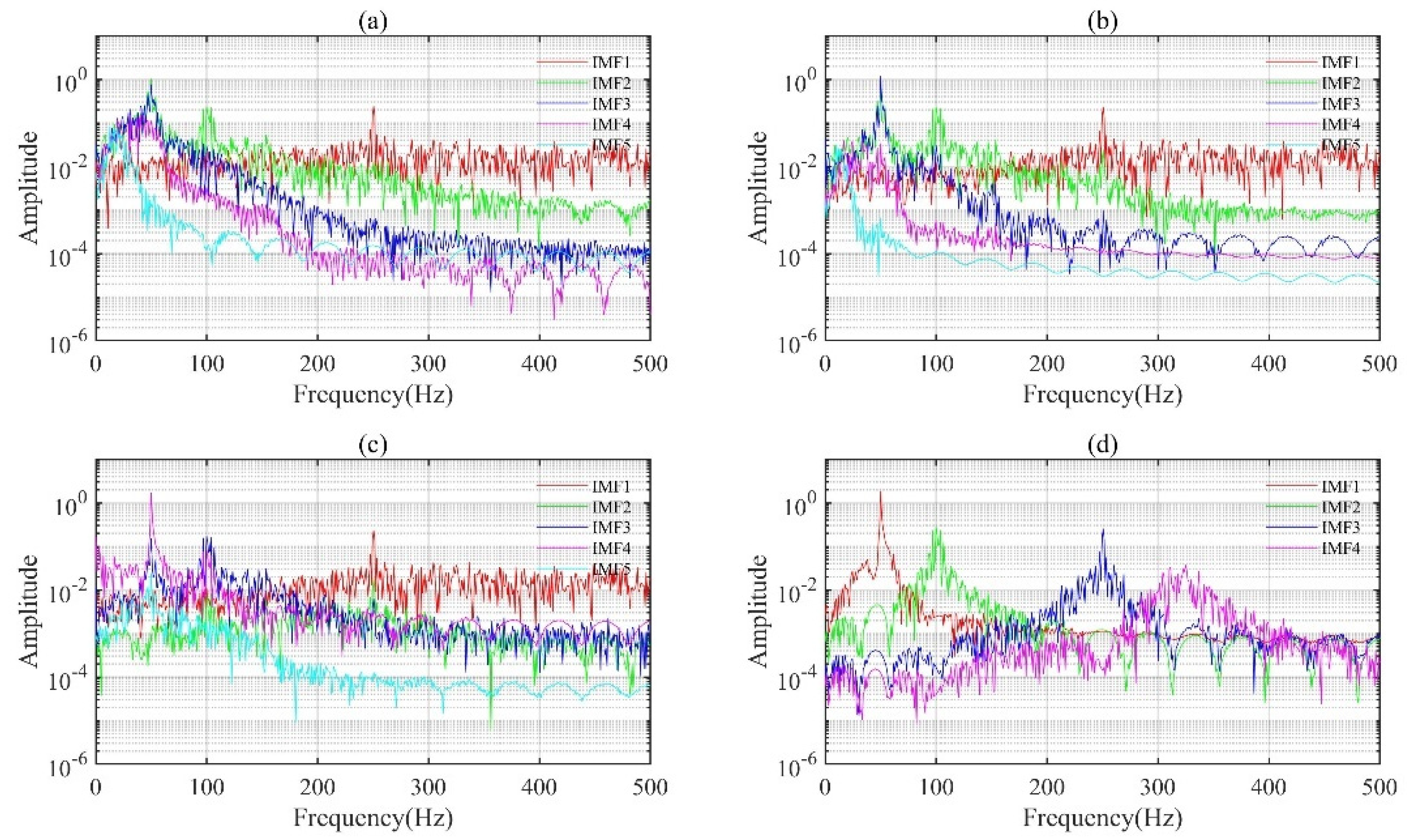
We synthesize a signal by 50 Hz, 100 Hz, 250 Hz sinusoidal waves, and Gaussian white noise. Then the synthesized signal is decomposed by EMD, EEMD, CEEMD, and VMD, respectively. The four decomposed IMFs are shown in the frequency domain in Figure 1. It can be seen clearly in Figure 1d that the VMD algorithm decomposes the frequency components of 50 Hz, 100 Hz, and 250 Hz into IMF1, IMF2, and IMF3 independently, which overcomes the mode−mixing problem. Compared with IMFs from VMD, more IMFs are decomposed by EMD, EEMD, and CEEMD methods, which show overlapped frequency ranges to some extent, as shown in Figure 1a–c.
2.2. The Optimization Algorithm for VMD Parameters α and K Based on PSO
Normally, the VMD algorithm decomposes the signal by manually pre−determining the number of IMFs K and the value of the penalty parameter . The smaller the value of is, the wider the bandwidths of the resulting IMFs are; the larger the value of K is, the narrower the bandwidths of the IMFs are. It is very important to determine these two parameters quickly and accurately as they affect the decomposition results directly. We apply the PSO algorithm to search the values of K and automatically in VMD processing.
The idea of the PSO algorithm originated from the foraging behavior of a flock of birds, where the flock finds the optimal destination by sharing information collectively [15]. Imagine a scenario in which a flock of birds randomly searches for food in a forest and they want to find the location with the largest amount of food. All the birds can only sense the approximate direction of the food, but they do not know exactly where the food is. Each bird searches in the direction it decides, and during the search, it records the location of the largest amount of food it has ever found and shares the location and amount of food with other birds so that all the birds can know where the largest amount of food is at present. During this process, each bird adjusts its search direction according to the location of the largest amount of food in its memory and records from the current flock. After a period of searching, the flock can find out the location of the largest amount of food in the forest, i.e., the global optimal solution is obtained.
The PSO algorithm first randomly initializes the particle swarm in a given space, and each particle has a fitness value corresponding to the objective function being optimized. Each particle decides the distance and direction of flight based on its individual experience and the experience of its neighbors so that the particle swarm searches for the optimal solution in the solution space from generation to generation with the current optimally located particles.
Let the population consisting of M particles in a D−dimensional space be , the position of the first particle is . The individual optimal position of each particle during the flight is , where the individual optimal position at which the first particle is , i.e., the individual local extremes. The optimal position of the g−th particle throughout the flight is , i.e., the population global extremum. The i−th particle travels at the speed of . The velocity and position of each particle flight are updated continuously and iteratively by the two extremums:
where ; ; are inertia weights; is the number of current iterations; are the acceleration constant; is a random number.
In this paper, we use the envelope entropy as the fitness function [17]. The smaller the envelope entropy is, the better the fitting is. The envelope entropy is calculated by
where signal is obtained from the signal by Hilbert transform, and is the normalized form of the envelope signal . can represent the sparsity of the original signal quantitatively. The smaller the value of is, the sparser the signal is, and the less noise it contains. Conversely, the larger the value of is, the weaker the signal sparsity is, and the more noise it contains.
After a certain is selected, are obtained through VMD decomposition. Then the value of each IMF component is calculated separately, and the smallest value among them is found as the local minimum entropy value. The is used as the fitness function, and the local minimal value is used as the search target.
The best search process in the VMD algorithm is summarized as follows:
(1) determine the initial parameters of the PSO and the envelope entropy as the fitness function;
(2) generate the positions of particles randomly in some particle populations and their velocities of movement;
(3) process the signal by VMD at different positions and calculate of the corresponding for each particle position;
(4) update individual local extremes and population global extremes through comparison of the magnitude of ;
(5) update the velocity and position of particles;
(6) loop the steps (3)−(5), then end the loop when the number of iterations reaches a threshold and outputs the best particle position .
To check the validity of the method, as an example, we synthesize a signal by Equation (7), including cosine signals of 5 Hz, 20 Hz, 40 Hz, 60 Hz, 80 Hz, 100 Hz, and 120 Hz, respectively.
The synthetic signal is decomposed by VMD, whose parameters are determined automatically by the PSO algorithm. The initial parameters of the PSO algorithm were set as follows: evolutionary generation of 10, the population size of 10, inertia weight of 1.5, and acceleration constant of 1.5 and 1.0, respectively. In the PSO algorithm, the inertia weight coefficient determines how much of the last iteration speed is retained. Choosing 1.5 as inertia weight is because a larger one can give the algorithm strong global search ability. The acceleration constant determines the size of the particle learning amount for the optimal position, and the optimal range of the acceleration constant is determined from 0.5 to 2.5 by the Benchmark function set.
The initial positions of the particles and their entropy value are shown in Figure 2a, where the color shows the entropy value. The minimum value of the local minimal entropy value 6.152145 appears in the 5th generation, as shown in Figure 2b, and the optimal combination of parameters obtained by the optimization search is , as shown in Figure 2c, which is marked in a red circle. The parameter-optimized VMD yields seven IMFs, whose waveforms are shown in Figure 3a−g and corresponding spectra in Figure 3h−n, respectively. IMFs 1−7 correspond to the frequency components of 5 Hz, 80 Hz, 120 Hz, 100 Hz, 60 Hz, 20 Hz, and 40 Hz, respectively. The synthetic example proves the effectiveness of PSO-based parameter−optimized VMD.
2.3. The Proposed GPR Data Denoising Method
As effective signal denoising and reconstruction method, VMD still suffers the problem of manually selecting the parameters like K . Based on the above study, a PSO-based VMD denoising method for the GPR profile is proposed here. The specific implementation steps are as follows when this method is applied to the real field data.
(1) We first pre−process GPR data using conventional methods like time-zero correction, direct current (DC) component removal, gain or automatic gain control (AGC), band-pass filtering et al., which can be selected on a case-by-case basis.
(2) Then the average trace of GPR data is obtained, for which the PSO algorithm is used to search for the best combination of parameters in the VMD.
(3) Next, the GPR data are decomposed trace by trace using VMD, and K IMFs from each trace are obtained. Therefore, the original GPR profile generates K profiles of IMF with different features.
(4) The last step is data reconstruction which is to select the useful IMF profiles for superposition so that the target signal is revealed by removing the useless IMFs which represent noise. How can we determine which IMFs are useful? Similarly, we abandon manual experience judgment and propose a gauging method based on SNR and RMSE.
The SNR and RMSE are calculated as follows:
where is the noise-containing signal, is the signal after noise reduction, N is the number of sampling points, and M is the number of traces. The higher SNR indicates that the more effective information is contained in the signal with a better noise reduction effect. RMSE is a measure of the deviation of the noise reduction signal from the mean value of the original data. The smaller the root mean square error is, the better the noise reduction effect is.
3. Application
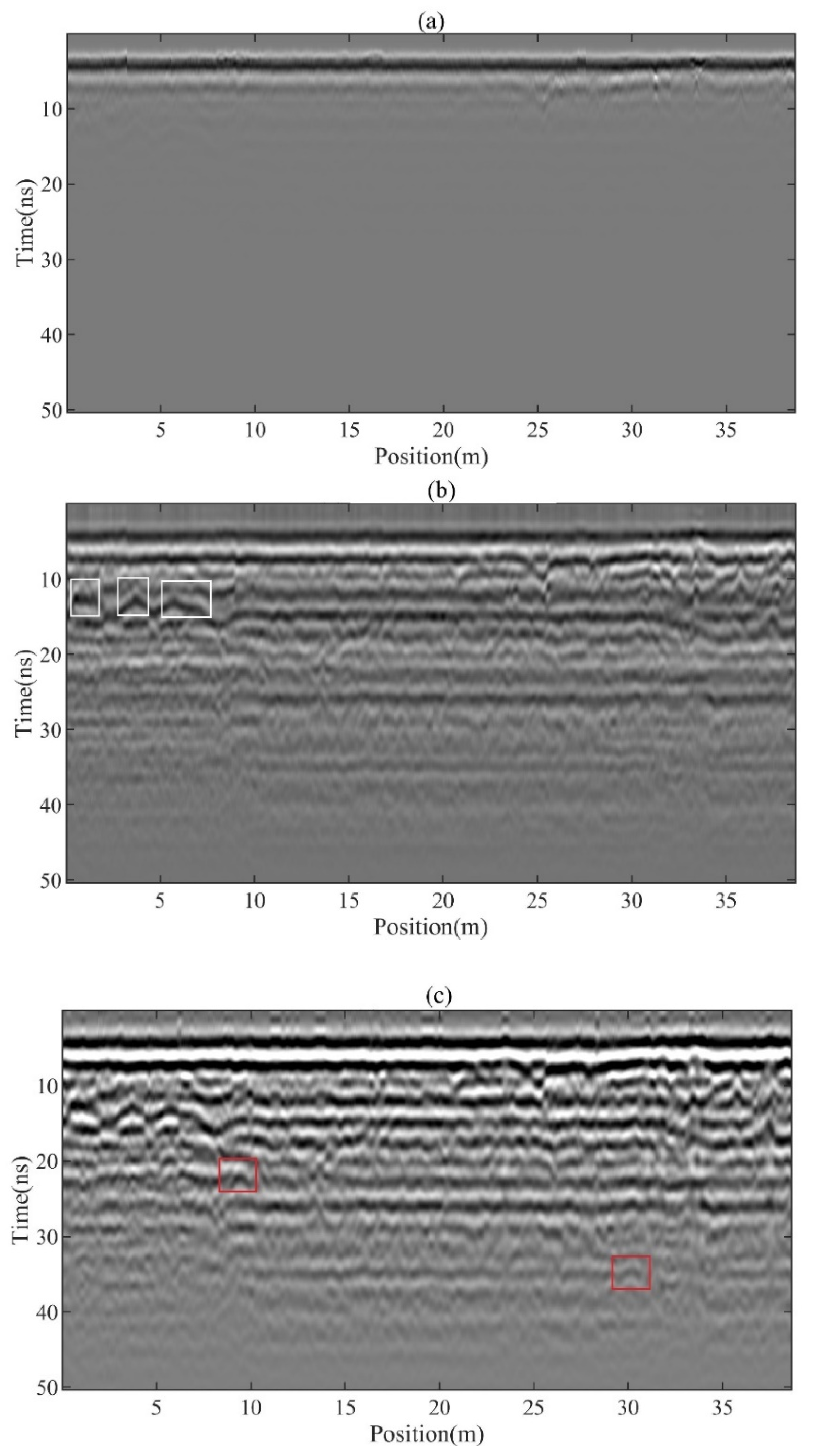
Figure 4a shows field data collected by a GPR system from MALA, Sweden, on the campus of Jilin Jianzhu University. Using the antenna with the central frequency of 500 MHz, a total of 782 traces are collected and there are 668 sampling points in each trace. The time step and the distance step are 0.0754 ns and 0.0494 m, respectively. It is difficult to find targets from the raw data shown in Figure 4a. Then the raw data are pre-processed with DC component removal, AGC, band−pass filtering, and moving average, while the related parameters are set as follows: (2) AGC window width is 10 ns, (2) the frequency band in band-pass filtering is between 99−550 MHz, (3) the number of points in moving average is 5. The pre−processed profile is shown in Figure 4b, from which it can be seen that the anomaly target signal is highlighted. There are three obvious stratigraphic interfaces at 15 ns, 25 ns, and 35 ns, respectively, and three point-like reflection events from underground pipes marked by white boxes at a position of 2 m around 12 ns, a position of 4 m around 12 ns, and a position of 5 m around 12 ns. However, the radar profile still contains some noise. The RMSE and SNR of the pre-processed data are 93.0751 and 7.5400 × 10³, respectively.
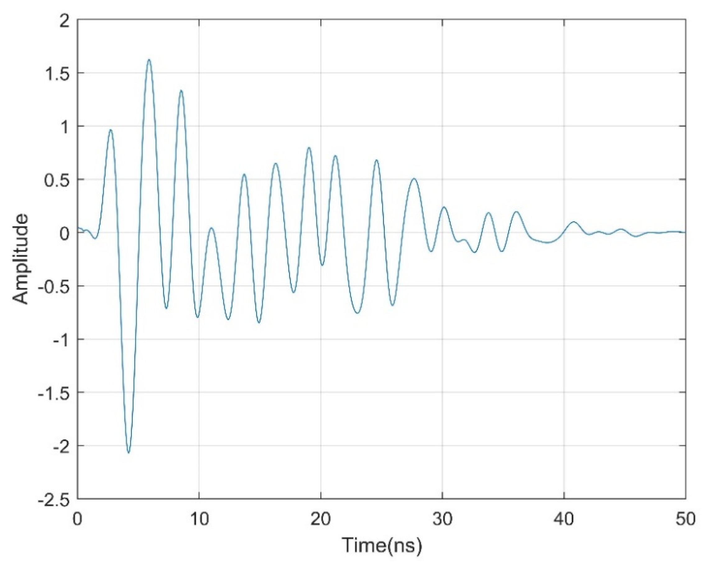
Figure 5 shows the average trace of the radar profile in Figure 4b, which is searched by the PSO algorithm for the best combination parameters . The determination of by PSO is shown in Figure 6. Figure 6a shows the initial position of the particles, and Figure 6b shows the change process of the local minimal entropy value with the number of generations of population evolution in the particle swarm optimization search process. The minimum value of the local minimum entropy value of 5.9981 appears in the 7th generation, and the optimal combination of parameters = [6, 2161]. Figure 6c shows the particle population distribution after evolution; the solid circle is the distribution of each particle, the color represents the entropy value, while the empty red circle marks the final selected point, corresponding to the optimal parameters.
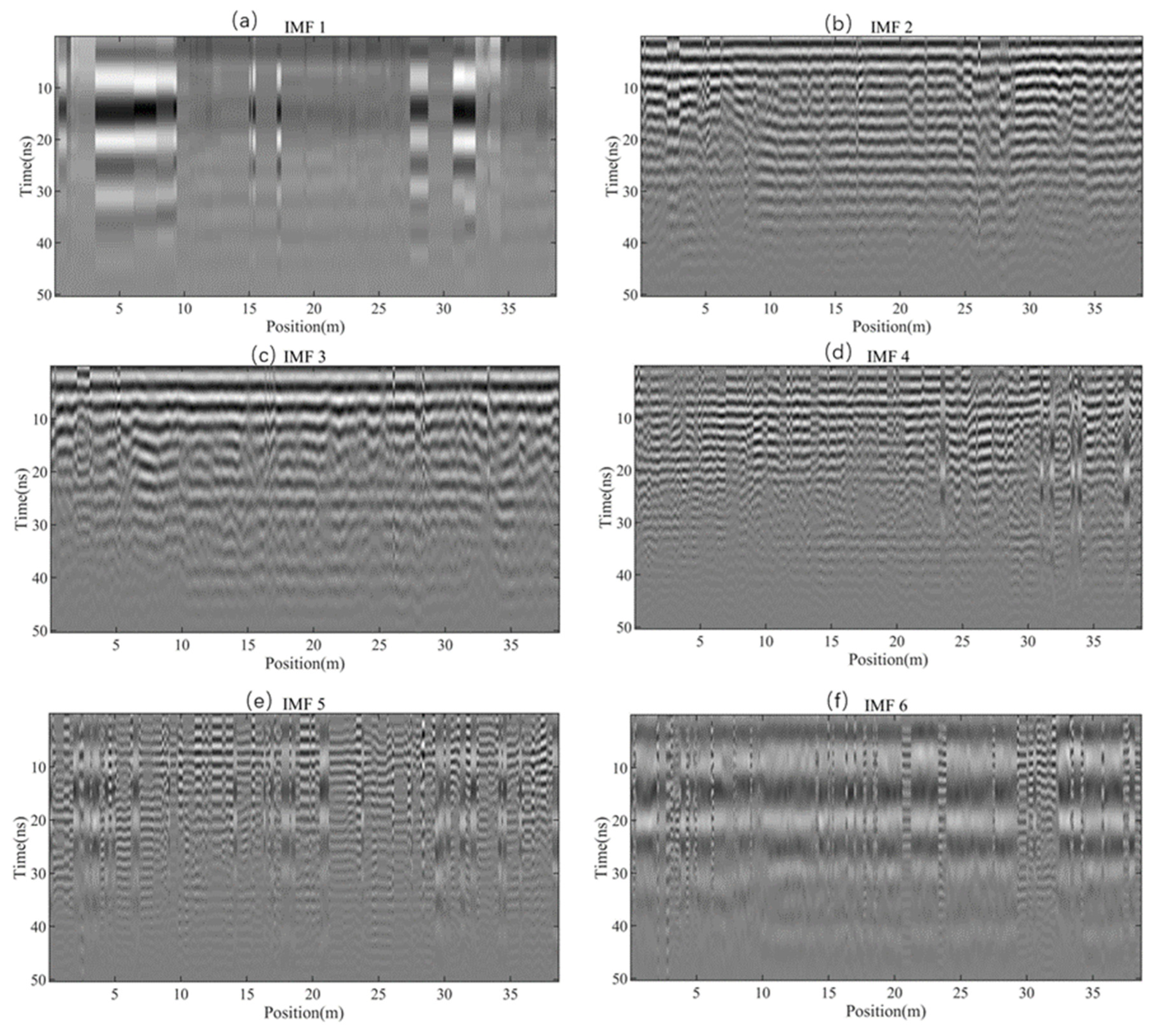
We use the optimal parameter for VMD processing. Figure 7 shows the 6 IMFs obtained after VMD decomposition, where IMFs 1 and 6 show low−frequency components, while IMFs 2, 3, 4, and 5 show relatively high−frequency components. By observing these 6 IMF profiles, it is intuitively difficult to judge which ones should be selected for data reconstruction. Our judgment is based on SNR and RMSE after superposition of different IMF profiles. The SNR and RMSE for superposition from different IMF profiles are calculated respectively according to Equations (8) and (9), and the results of the SNR and RMSE are listed in Table 1. From the values of SNR and RMSE, it can be seen that the smallest RMSE, 84.2721, and the largest SNR, 4.4886 × 10³ correspond to the combination of IMFs 2, 3, 4, which is selected as the best superposition, and the other combinations are also significantly better than the combination including IMF5 or IMF6. The reconstructed profile of the superposition of IMFs 2, 3, and 4 are shown in Figure 4c. Compared with the pre-processed data, the reconstructed data shows larger SNR and smaller RMSE. From Figure 4c, it can be clearly seen that the three point−like reflection events and the stratigraphic interfaces. Besides these, two point−like reflection events from underground pipes are revealed at a position of 30 m around 35 ns, and a position of 10 m around 20 ns, which are marked by red boxes.
The purpose of the investigation is to find unknown underground pipelines for further land use. According to Figure 4c, we described the stratigraphic distribution and the location of pipelines, which is shown in Figure 8. Four layers interpreted are artificial fill for plant growth, constructive waste, unknown material, and the original soil, respectively. Five pipelines are located in red circles. The discontinuities of two bottom layer interfaces can be found between 30 to 35 m.
4. Conclusions
Compared with EMD, EEMD, and CEEMD, VMD can obtain sparser and band-limited IMFs, which better match the intrinsic characteristics of signals. The number of IMFs, K, and penalty parameters, , are the key parameters that directly affect the decomposition results of VMD, but the determination of their values relies on manual judgment. In this paper, we proposed a method to automatically search K and by the PSO algorithm used in VMD processing to reduce uncertainty due to subjective judgment. We test the method by a synthetic signal, which shows that it can find K and quickly and accurately. Similarly, to select IMFs for data reconstruction without manual judgment, we then propose a judgment method based on SNR and RMSE; that is, to find those IMFs, their superposition gives the maximum SNR and minimum RMSE. We show the utility of this process of automatic parameter search and data reconstruction on field data. The noises are suppressed and targets are identified clearly in reconstructed data. The proposed method of automatic judgment overcomes the deficiency of relying on manual experience and suppresses noise effectively without reducing efficiency. In the future, we will further improve the optimal combination algorithm of IMFs to increase efficiency.
Author Contributions
Conceptualization, S.L. and Q.L.; methodology, S.L., C.L. and Q.L.; Formal analysis, Y.C., H.J. and H.L. (Hongqing Li); data curation, H.L. (Hong Li) and C.L.; writing—original draft preparation, S.L., Y.C. and Q.L.; writing—review and editing, S.L. and Q.L.; funding acquisition, S.L. and C.L. All authors have read and agreed to the published version of the manuscript.
Funding
This research was funded by Science and Technology on Near−Surface Detection Laboratory under Grant 6142414200606.
Conflicts of Interest
The authors declare no conflict of interest.
References
- Jol, H. Ground Penetrating Radar: Theory and Applications; Elsevier Science: Amsterdam, The Netherlands, 2009. [Google Scholar]
- Daniels, D.J. Ground Penetrating Radar, 2nd ed.; The Institution of Engineering and Technology: London, UK, 2004. [Google Scholar]
- Huang, N.; Shen, Z.; Long, S.; Wu, M.; Shih, H.; Zheng, Q.; Yen, N.; Tung, C.; Liu, H. The empirical mode decomposition and the Hilbert spectrum for nonlinear and non-stationary time series analysis. Proc. Math. Phys. Eng. Sci. 1998, 454, 903–995. [Google Scholar] [CrossRef]
- Song, E.; Liu, S.; Lu, Q.; Wang, X.; He, R. A moving target detection method based on Kalman filter and EMD for Through-Wall Radar. In Proceedings of the CGS/SEG International Conference, Qingdao, China, 17–20 April, 2017. [Google Scholar]
- Ostoori, R.; Goudarzi, A.; Oskooi, B. GPR random noise reduction using BPD and EMD. J. Geophys. Eng. 2018, 15, 347–353. [Google Scholar] [CrossRef]
- Wu, Z.; Huang, N. Ensemble empirical mode decomposition: A noise-assisted data analysis method. Adv. Adapt. Data Anal. 2009, 1, 11–41. [Google Scholar] [CrossRef]
- Chen, C.; Jeng, Y. Nonlinear data processing method for the signal enhancement of GPR data. J. Appl. Geophys. 2011, 75, 113–123. [Google Scholar] [CrossRef]
- Torres, M.E.; Colominas, M.A.; Schlotthauer, C.; Flandrin, P. A complete ensemble empirical mode decomposition with adaptive noise. In Proceedings of the IEEE International Conference on Acoustics Speech and Signal Processing (ICASSP), Prague, Czech Republic, 22–27 May 2011; pp. 4144–4147. [Google Scholar]
- Manataki, M.; Sarris, A.; Vafidis, A. Combining CEEMD and Predictive Deconvolution for the Suppression of Multiple Reflections and Coherent Noise in GPR Signals. In Proceedings of the 8th International Workshop on Advanced Ground Penetrating Radar (IWAGPR), Florence, Italy, 7–10 July 2015. [Google Scholar]
- Li, J.; Liu, C.; Zeng, Z.; Chen, L. GPR Signal Denoising and Target Extraction with the CEEMD Method. IEEE Geosci. Remote Sens. Lett. 2015, 12, 1615–1619. [Google Scholar]
- Dragomiretskiy, K.; Zosso, D. Variational Mode Decomposition. IEEE Trans. Signal Processing 2014, 62, 531–544. [Google Scholar] [CrossRef]
- Zhang, X.B.; Nilot, E.; Feng, X.; Ren, Q.C.; Zhang, Z.J. IMF-Slices for GPR Data Processing Using Variational Mode Decomposition Method. Remote Sens. 2018, 10, 476. [Google Scholar] [CrossRef] [Green Version]
- Xu, J.; Lei, B. Data Interpretation Technology of GPR Survey Based on Variational Mode Decomposition. Appl. Sci. 2019, 9, 2017. [Google Scholar] [CrossRef] [Green Version]
- He, W.; Hao, T.; Je, H.; Zheng, Q.; Lin, K. Joint time-frequency analysis of ground penetrating radar data based on variational mode decomposition. J. Appl. Geophys. 2020, 181, 104146. [Google Scholar] [CrossRef]
- Kennedy, J.; Elberhart, R. Particle swarm optimization. In Proceedings of the IEEE International Conference on Neural Networks, Perth, Australia, 27 November–1 December 1995; pp. 1942–1948. [Google Scholar]
- Mezura-Montes, E.; Coello Coello, C.A. Constraint-handling in nature-inspired numerical optimization: Past, present and future. Swarm Evol. Comput. 2011, 1, 173–194. [Google Scholar] [CrossRef]
- Tang, G.; Wang, X. Parameter optimized Variational Mode Decomposition method with application to incipient fault diagnosis of rolling bearing. J. Xi’an Jiaotong Univ. 2015, 49, 73–81. [Google Scholar]
Figure 1.
The frequency spectrums of different IMFs after decomposition by different methods: (a) EMD, (b) EEMD, (c) CEEMD, and (d) VMD.
Figure 1.
The frequency spectrums of different IMFs after decomposition by different methods: (a) EMD, (b) EEMD, (c) CEEMD, and (d) VMD.

Figure 2.
Determination of the optimal combination of by PSO for the synthetic signal. (a) Initial position of the particles, (b) The change of local minimum entropy value with PSO evolution, and (c) the final position of the particles with the optimum value is marked in the red circle.
Figure 2.
Determination of the optimal combination of by PSO for the synthetic signal. (a) Initial position of the particles, (b) The change of local minimum entropy value with PSO evolution, and (c) the final position of the particles with the optimum value is marked in the red circle.

Figure 3.
The decomposed IMFs (a–g) and their corresponding spectra (h–n) by PSO based parameter-optimized VMD for the synthetic signal.
Figure 3.
The decomposed IMFs (a–g) and their corresponding spectra (h–n) by PSO based parameter-optimized VMD for the synthetic signal.

Figure 4.
The comparison of GPR profile of different steps: (a) raw data, (b) after pre-processing, and (c) after VMD reconstruction.
Figure 4.
The comparison of GPR profile of different steps: (a) raw data, (b) after pre-processing, and (c) after VMD reconstruction.

Figure 5.
The averaged trace from pre−processing GPR data.

Figure 6.
Determination of the optimal combination of by PSO for the average trace in Figure 5. (a) Initial position of the ten particles, (b) The change of local minimum entropy value with population evolution generation, (c) the final position of the particles with the optimum value is marked in the red circle.

Figure 7.
IMFs after VMD decomposition: (a–f) show IMF1−IMF6, respectively.

Figure 8.
Interpretation for Figure 4c. Four layers are described and the locations of five pipelines are marked by red circles.
Figure 8.
Interpretation for Figure 4c. Four layers are described and the locations of five pipelines are marked by red circles.


Table 1.
RMSE and SNR of different IMFs combinations.
| No. | IMFs | RMSE | SNR | Note |
|---|---|---|---|---|
| 1 | 1-6 | 94.3715 | 2.7131 × 10³ | |
| 2 | 1-5 | 92.9000 | 2.9594 × 10³ | |
| 3 | 2-6 | 91.0887 | 3.2669 × 10³ | |
| 4 | 2, 3, 4, 5 | 88.5110 | 3.7170 × 10³ | |
| 5 | 2, 3, 4 | 84.2721 | 4.4886 × 10³ | Selected |
| 6 | 3, 4, 5 | 93.8490 | 2.8074 × 10³ | |
| 7 | 2, 4, 5 | 92.2973 | 3.0711 × 10³ | |
| 8 | 2, 3, 5 | 86.5641 | 4.0683 × 10³ |
Publisher’s Note: MDPI stays neutral with regard to jurisdictional claims in published maps and institutional affiliations. |
© 2022 by the authors. Licensee MDPI, Basel, Switzerland. This article is an open access article distributed under the terms and conditions of the Creative Commons Attribution (CC BY) license (https://creativecommons.org/licenses/by/4.0/).
Share and Cite
MDPI and ACS Style
Liu, S.; Chen, Y.; Luo, C.; Jiang, H.; Li, H.; Li, H.; Lu, Q. Particle Swarm Optimization-Based Variational Mode Decomposition for Ground Penetrating Radar Data Denoising. Remote Sens. 2022, 14, 2973. https://doi.org/10.3390/rs14132973
AMA Style
Liu S, Chen Y, Luo C, Jiang H, Li H, Li H, Lu Q. Particle Swarm Optimization-Based Variational Mode Decomposition for Ground Penetrating Radar Data Denoising. Remote Sensing. 2022; 14(13):2973. https://doi.org/10.3390/rs14132973
Chicago/Turabian StyleLiu, Sixin, Yuhan Chen, Chaopeng Luo, Hejun Jiang, Hong Li, Hongqing Li, and Qi Lu. 2022. "Particle Swarm Optimization-Based Variational Mode Decomposition for Ground Penetrating Radar Data Denoising" Remote Sensing 14, no. 13: 2973. https://doi.org/10.3390/rs14132973
Note that from the first issue of 2016, this journal uses article numbers instead of page numbers. See further details here.