
Deformation Monitoring of Tailings Reservoir Based on Polarimetric Time Series InSAR: Example of Kafang Tailings Reservoir, China

Key Laboratory of Land Environment and Disaster Monitoring, Ministry of Natural Resources, China University of Mining and Technology, Xuzhou 221116, China
*
Author to whom correspondence should be addressed.
Remote Sens. 2022, 14(15), 3655; https://doi.org/10.3390/rs14153655
Submission received: 30 June 2022
/
Revised: 23 July 2022
/
Accepted: 27 July 2022
/
Published: 29 July 2022
(This article belongs to the Special Issue Distributed Spaceborne SAR: Systems, Algorithms, and Applications)
Abstract
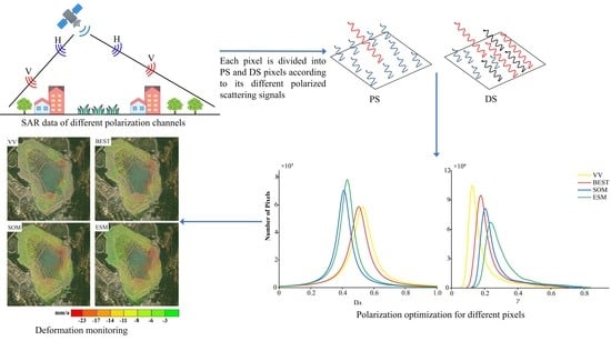
:Safe operation of tailings reservoirs is essential to protect downstream life and property, but current monitoring methods are inadequate in scale and refinement, and most reservoirs are built in low coherence areas far from cities. Use of polarization data to monitor deformation may improve area coherence and thus point selection density. With the example of the Kafang tailings reservoir and dual-polarization Sentinel-1 data from 9 August 2020 to 24 May 2021, homogeneous points of different polarization channels were identified with the hypothesis test of the confidence interval method. Results were fused, and BEST, sub-optimum scattering mechanism (SOM), and equal scattering mechanism (ESM) methods were used to optimize phase quality of persistent scatterer (PS) and distributed scatterer (DS) pixels and obtain more detailed deformation information on the area with time series processing. The fusion of homogeneous point sets obtained from different polarization intensity data increased the number of homogeneous points, which was 3.86% and 8.45% higher than that of VH and VV polarization images, respectively. The three polarization optimization methods improved point selection density. Compared with the VV polarization image, the high coherence point density increased by 1.83 (BEST), 3.66 (SOM), and 5.76 (ESM) times, whereas it increased by 1.17 (BEST), 1.84 (SOM), and 2.04 (ESM) times in the tailings reservoir. The consistency and reliability of different methods were good. By comparing the monitoring results of the three methods using polarization data, the hypothesis test of the confidence interval (HTCI) algorithm, and the polarization optimization method will effectively increase the point selection number of the study area, and the ESM method can show the deformation of tailings area more comprehensively. Monitoring indicated deformation of the tailings reservoir tended to diffuse outward from the area with the largest deformation and was relatively stable.
1. Introduction
Tremendous amounts of tailings which cannot be reused and cleaned in the short term usually accumulate in tailings reservoirs. According to incomplete statistics, global production exceeds 10 billion tonnes of tailings per year [1], and with development of the mining industry, tailings output is expected to increase further. However, accumulations of tailings have high gravitational potential energy [2]. When an accidental dam break occurs, debris flows form easily and seriously damage the environment surrounding a mining area. In the past decade, several accidental dam breaks of tailings reservoirs have occurred worldwide. For example, in 2008, the dam holding the Xinta mine tailings reservoir in Xiangfen County, Shanxi Province, China, broke, and the resulting debris flow instantly flooded the downstream, causing 281 deaths and 33 injuries [3]. In 2014, the Canadian Matt Poligin tailings reservoir accident dumped approximately 25 billion liters of tailings into Polly Lake, Bonzi Creek, and Quesnel Lake, seriously damaging the local environment [4]. In 2019, Vale’s tailings reservoir in Brumadinho City, Brazil collapsed, and approximately 12 million cubic meters of tailings poured into the Paraopeba River, causing more than 240 deaths and unknown economic losses [5]. Therefore, it is particularly important to monitor deformation of tailings reservoirs as well as surrounding surfaces.
In most current research, the level, total station, global navigation satellite system, and sensors are used to obtain the deformation of some points on a tailings reservoir. However, it is difficult to obtain high-precision and fine-scale deformation monitoring of tailings reservoirs with high efficiency. With the development of time series interferometric synthetic aperture (InSAR) technology, persistent scatterers InSAR (PS-InSAR) [6], small baseline subset InSAR (SBAS-InSAR) [7], and temporary coherent point InSAR (TCP-InSAR) [8] have been widely used to monitor various types of surface deformation. Iannacone et al. [9] used Sentinel-1 satellite images with differential InSAR (D-InSAR) and Multi-Temporal InSAR to monitor the deformation of a tailings reservoir in Chile and found 80 mm of deformation from October 2014 to January 2018. Gamma et al. [10] used PS-InSAR and SBAS to monitor deformation of the Brumadinho tailings reservoir and analyzed the causes of deformation in combination with local precipitation data. Mazzanti et al. [11] used D-InSAR to monitor deformation of the Zelazny Most tailings reservoir and found a maximum deformation rate of −30 mm/year. The authors used relevant literature to analyze causes of deformation. Although previous studies demonstrated approaches to improve deformation monitoring of tailings reservoirs, it is impossible to obtain more comprehensive and detailed information on deformation of tailings reservoirs because of insufficient density of monitoring points.
Both traditional time series InSAR and distributed scatterers InSAR (DS-InSAR) [12] use only the intensity and phase information of SAR images, and the polarization information is often ignored. Because different ground objects reflect different radar electromagnetic waves, single polarization can only indicate the reflection information of some ground objects. Therefore, fusion of different polarization information can increase the amount of surface information obtained. Applying fused polarization information to monitor time series surfaces and man-made structures can increase the density of monitoring points and obtain more detailed deformation information. Navarro et al. [13] showed that using polarimetric capabilities improves the selection density and phase quality of stable pixels in PS-InSAR. Iglesias et al. [14] used amplitude dispersion () and coherence () as the phase quality metric, and three different polarization optimization methods were used to monitor landslides and deformation in Barcelona City. Sadeghi et al. [15] proposed a method to increase the number of PS points using time coherence polarization optimization of PS points in a polarimetric Stanford method for persistent scatterers (PolStaMPS) technology, which successfully applied polarization information to surface deformation monitoring of the Tehran Basin. Mullissa et al. [16] proposed a polarization time series method based on distributed targets and found that the method could significantly increase the point selection density in the monitoring area, with the increase nearly eight times higher than that with the single-polarization channel. Zhao et al. [17] employed the amplitude dispersion index (PolPSI-ADI) and coherence (PolPSI-COH) as the phase quality metric and took adaptive optimization strategies for different kinds of SAR pixels (PolPSI-AOS) to conduct experiments based on dual polarization Sentinel data in Beijing, Fukang, and Xinjiang and XiaoLangDi, respectively, which are three areas with different land cover, and described in detail the advantages and disadvantages of each according to the comparison results.
However, tailings reservoirs are mostly built far from cities, and therefore, loss of coherence can easily occur in SAR images. As a result, there is relatively low point selection density in a traditional time series InSAR method, which affects the accuracy and detail of deformation monitoring. Therefore, to obtain more detailed deformation information on a tailings reservoir, polarization information was introduced into the processing of time series InSAR data, and PS and DS pixels were combined in this study. The approach will provide a new level of technical support for the safe operation of tailings reservoirs.
After the introduction, the Section 2 of the paper introduces the research area. The Section 3 introduces the basic principles of the homogeneous point identification method and the three polarization optimization methods of BEST, SOM, and ESM. In the Section 4, optimization results are evaluated, and monitoring results of a tailings reservoir are analyzed. The Section 5 and Section 6 are discussion and conclusions, respectively.
2. Experimental Area and Data
2.1. Experimental Area
The mining industry has a long history in Gejiu City, Yunnan Province, China, that began more than 2000 years ago [18]. The region is rich in mineral resources, and discovered reserves of tin, copper, zinc, and other ores are estimated at 6.5 Mt. In particular, reserves of tin are as high as 0.9 Mt, accounting for approximately 33.3% of total tin reserves in China [19]. The area produces the most tin in China and was the earliest tin production site worldwide [20]. After years of ore mining, many tailings reservoirs have been built in the area. The focus in this paper was the Kafang tailings reservoir with geographic coordinates of – E, – N operated and managed by the Yunxi Kafang branch (Figure 1).
The Kafang tailings reservoir is a flat, third-class tailings reservoir, which is at the junction of the central Yunnan fold belt, Yangzi platform, and Simao block [21]. The reservoir is formed by the merger of Yuanxiniu Pond and Yangmei Mountain and Yueya Pond tailings reservoirs. The mining area covers 913,000 m2, and the design storage capacity is 18.53 million m3. By 2020, 10 million tons of tailings had accumulated in the tailings reservoir [22]. After years of ore mining in the area, a total of eight sub-dams have been built in the Kafang tailings reservoir area to form a circular tailings reservoir. Tailings accumulated in the reservoir are discharged into the tailings reservoir along the crest of the surrounding stacking dams, forming a circular alternating ore drawing mode. In addition, the downstream of the tailings reservoir is adjacent to the plant area of the Kafang branch of the Yunnan Tin Group and Kafang Town. It is a typical “overhead reservoir” [23]. When a dam break accident occurs, the high gravitational potential energy of tailings in a tailings reservoir is converted into kinetic energy, causing a major debris flow disaster with tremendous damage to the environment and people in its path. Therefore, it is vital to realize large-scale, accurate, and reliable deformation monitoring of tailings reservoirs to ensure safe operation.
2.2. Experimental Data
The Sentinel-1 earth observation satellite launched by the European Space Agency Copernicus program provides users with dual-polarization (VV-VH, HH-HV) or single polarization data (HH, VV) free of charge. In this paper, the experimental data were 25 dual-polarization, C-band Sentinel-1 SAR images covering the Kafang tailings reservoir, and the time span was from 9 August 2020 to 24 May 2021. Satellite images adopted terrain observation with progressive scans SAR (TOPSAR) imaging mode, VV-VH polarization, incident angle of 43.98°, and range and azimuth pixel sizes of 2.33 and 13.95 m, respectively, and the image time resolution was 12 days.
In addition, the external digital elevation model used the 30-m resolution Shuttle Radar Topography Mission (SRTM) provided by the National Aeronautics and Space Administration and the National Imagery and Mapping Agency to remove the terrain phase in the interference phase.
3. Method
3.1. Statistically Homogeneous Point (SHP) Identification
Although fast statistically homogeneous pixel selection (FaSHPS) [24] overcomes the problem that the traditional hypothesis test is inefficient in identifying homogeneous points to some extent, the algorithm does not effectively reject nonhomogeneous pixels. Therefore, Jiang et al. [25,26] improved the FaSHPS algorithm on the basis of sample characteristics of homogeneous points and proposed using the intensity mean of homogeneous pixels in the local window to determine a more accurate confidence interval. The HTCI method increases the efficiency of homogeneous point recognition.
Suppose there is a SAR image set () with N scenes subject to a complex circular Gaussian distribution, whose variance is , and the intensity of any pixel in the time dimension follows an exponential distribution:
Under the assumption of a complex circular Gaussian distribution, whether the reference pixel () and the pixel to be estimated () are homogeneous points can be expressed by Equation (2).
where and are the null hypothesis and the alternative hypothesis, respectively. The algorithm first replaces the intensity of the reference pixel with the mean intensity of the reference pixel in the time dimension ().
Because a likelihood ratio test (LRT) can effectively control the first type of error of a hypothesis test, the initial set of homogeneous points of reference pixels can be identified by this method in a small window. Then, under the condition of 2N degrees of freedom, the following Equation (3) can be obtained according to the relation between exponential and chi-square distributions ():
Therefore, when the reference pixel and the pixel to be estimated belong to the homogeneous point, that is, it is true, the ratio of the average intensity of the reference pixel and the pixel to be estimated obeys the F distribution, and its confidence interval is the following:
The initial set of homogeneous points of the reference pixel is obtained by Equation (4), and the average intensity of all homogeneous points in the set is used to replace the average intensity estimation of the reference pixel (). Because SAR image intensity is subject to a gamma distribution, a more accurate confidence interval for homogeneous point recognition can be obtained under a given confidence level using Equation (5):
where is the quantile of gamma distribution, is replaced by the average intensity estimation of the reference pixel, is replaced by the average intensity of the pixel to be estimated, and N is the number of SAR images. When the average intensity of the pixel to be estimated falls within the confidence interval, it is recognized as a homogeneous point. Otherwise, it is a heterogeneous point. This method successfully applies an LRT test to identify homogeneous points. On the basis of controlling the first type of error, the influence of the second type of error on the identification of homogeneous points is reduced.
3.2. Polarimetric Interferometry
Because dual-polarization (VV-VH) Sentinel-1 polarization data were used in this paper, [27] under the condition of backscattering reciprocity, so the scattering matrix can be expressed by Equation (6):
where and are vertical copolar and cross-polar channels, respectively. By using the unitary transformation [28], the scattering matrix can be transformed into the scattering matrix on any elliptic orthogonal basis .
where is transpose operator, and is the transformation matrix. The transformation matrix can be obtained from Equation (8):
where and are the orientation and ellipticity angles of the polarization ellipse, respectively, and is the absolute phase, which is irrelevant from the interferometric point of view and is generally set to 0.
The scattering vector k can be obtained by decomposing the scattering matrix S according to the Pauli basis [29]:
With two different scattering vectors and , the polarimetric SAR interferometry (PolInSAR) vector K can be obtained as follows [29]:
Under the assumption of spatial uniformity and ergodicity, the PolInSAR coherency matrix [30] can be obtained according to Equation (11):
where is the conjugate transpose, and are the coherency matrix of each polarimetric SAR (PolSAR) data set, and and are the PolInSAR coherency matrices. The normalized complex projection vector [31] is used to project the scattering vector as follows:
where is the scattering mechanism, and is the phase relation of the scatterer. Equation (13) is used to project the dual-polarization SAR image as follows:
where is the conjugate transpose, and is the scattering coefficient. When the normalized complex projection vector is determined, the interference phase generated by any two scattering vectors can be obtained by Equation (14) [32].
where arg () is the phase operator.
3.3. Polarimetric Optimization
To apply polarization information to deformation monitoring, BEST, ESM, and SOM polarization optimization methods were used to optimize PS and DS pixels to improve the phase quality, phase unwrapping accuracy, and monitoring point selection density.
3.3.1. BEST
The BEST method is based on the selected polarization channel, and it provides the highest coherence for each pixel of an interferogram [33]. After DS pixels are identified by the HTCI method, on the basis of BEST, the polarization of PS and DS pixels is optimized by using and , respectively.
To prevent phase mutation after polarization optimization, the same polarization channel should be selected for each interferogram, whether PS or DS pixels, to ensure phase stability. For PS and DS pixels, the and of each polarization channel are calculated, respectively, and the phase provided by the polarization channel that provides and is selected as the phase after polarimetric optimization as follows:
where and are the amplitude dispersion of copolar and cross-polarization, respectively, and are the coherence of copolar and cross polarization, respectively, and and are the minimum amplitude dispersion and the maximum coherence, respectively.
3.3.2. ESM
Because the BEST method only selects the phase that provides the minimum amplitude dispersion and the maximum coherence from the polarization channels as the optimized phase, it does not fully use the polarization information. Therefore, to make full use of polarization information in phase optimization, the equal scattering mechanism (ESM) method has been proposed [34].
This ESM method solves the projection vector and obtains the parameters that minimize and maximize the polarization amplitude dispersion () of PS pixels and the polarization average coherence () of DS pixels, respectively, as follows:
where and are the amplitude standard deviation and the mean amplitude of the pixel time series, respectively, makes the polarization amplitude dispersion and average coherence reach the minimum or maximum normalized complex projection vector, respectively, and N and n are the number of images and interferograms, respectively. There are many methods to solve parameters, but the commonly used method is currently exhaustive search polarization optimization [35]. The method traverses the entire polarization space to obtain the optimal projection vector . Because the optimal projection vector is not unique, the phase jump is prevented by Equation (17) as follows:
Physically, there is no time or scattering decoherence for the scatterers.
3.3.3. SOM
Although ESM makes full use of polarization information, it is only tenable under the assumption of polarization stability. Otherwise, abnormal values appear in the polarization optimization process, which render ESM results meaningless. Therefore, to avoid this situation, the sub-optimum scattering mechanism (SOM) method has been proposed [36].
Based on the concept of BEST, all combinations of and are searched to obtain the minimum amplitude dispersion and maximum coherence values, which are regarded as the optimal parameters, according to the following equations:
where and are determined as follows:
where and are the copolar and cross-polar channels under the parameters and , respectively, and is the first and second image, respectively, of the generated interferogram. The optimal parameters and are obtained by the equations in (18), and then the optimized interference phase is obtained. Because the solution space of this method is a subspace of ESM, the SOM method can effectively reduce the occurrence of outliers when polarization is unstable.
The above is the principle of the technology and method used in this paper, and the specific processing process is shown in Figure 2.
4. Experimental Results
According to the basic principle of PS-InSAR, a short spatiotemporal baseline can reduce the effect of SAR image decoherence [6]. In this paper, the image of 12 January 2021 in the center of the time series was selected as the main image, and the other images formed 24 interference pairs with the main image (Figure 3).
4.1. Analysis of Homogenous Point Selection
The selection of homogeneous points is a key step in the processing of polarization time series. Because different ground objects have different scattering mechanisms for electromagnetic waves with different polarization modes, it is difficult to fully identify homogeneous pixels through single polarization channels. Therefore, in this paper, multi-polarization information was used to extract homogenous points. The HTCI algorithm was used to select homogenous points at significance level = 0.05. A small 7 × 7 window was used to select the initial set of homogenous points, and then a large 15 × 15 window was used to determine the final set of homogenous points. The threshold of homogenous points was set to 20 [37]. The homogeneity selection results of VV (Figure 4a) and VH (Figure 4b) different polarization channels were fused as the final homogeneity recognition results (Figure 4c), and pixels were divided into PS and DS pixels according to the homogeneity threshold. Because of the fusion of homogeneous points of different polarization channels, some PS pixels can be easily mistakenly classified as DS pixels. Therefore, in this paper, the amplitude dispersion of each pixel in the DS set under different polarization channels was calculated, and the pixels with a value less than 0.25 [17] were classified as PS pixels.
As shown in Figure 4, in the area of vegetation coverage and tailings reservoir, the number of homogeneous points after fusion increased significantly. In addition, contours of features in the fusion results were more definitive, especially on lakes, roads, and the dam body of the tailings reservoir (areas A, B, and C, respectively; Figure 4), and the characteristics of those features were clearly identified. According to visual interpretation and statistical analysis, the most homogeneous points were identified with VH + VV, which increased the number by 8.45% and 3.86% compared with VV and VH, respectively (Table 1).
To demonstrate the advantages of the fusion method in identifying homogeneous points, three reference points, a, b, and c, were selected in areas A, B, and C (see Figure 4c), respectively, and the window to identify homogeneous points was set to 15 × 15 (Figure 5).
Different ground objects had different scattering characteristics of radar electromagnetic waves, which led to differences in the number of homogeneous points obtained from different polarization intensity image sets (Figure 5). As shown in Figure 5a,b, the proposed method effectively increased the number of homogeneous points selected from the reference pixel, whether in a region with strong or weak scattering intensity. On the exposed road (Figure 5b), the number of homogeneous points with the VH channel was similar to that with the VV channel, but by combining the identification results of the two homogeneous point data sets, the number of homogeneous points in the lower half of the road was effectively supplemented. In the tailings reservoir area (Figure 5c), the method also effectively increased density and accuracy of the selected homogeneous points.
Thus, the method of selecting homogeneous points used in this paper was reasonable and reliable. Next, according to identified homogeneous points, the threshold of homogeneous points was set to divide pixels into PS and DS pixels, and the polarization phase was optimized.
4.2. Polarimetric Optimization
The BEST, SOM, and ESM methods were used to optimize the polarization phase of the PS and DS pixels identified in the previous step. The original VV polarization and the optimized amplitude dispersion and coherence results were determined. Figure 6 shows distribution histograms of amplitude dispersion, and Figure 7 shows distribution histograms of coherence.
Amplitude dispersion was the phase quality index, and BEST, SOM, and ESM were used to optimize the PS pixels (Figure 6). The three methods effectively reduced the amplitude dispersion of PS, although effects of SOM and ESM were better than that of BEST, with ESM having the best effect. To further analyze effects, a local, enlarged view was examined (Figure 6b). Generally, the largest number of pixels with amplitude dispersion in the range of 0 to 0.45 was after ESM optimization, followed by that after SOM and then BEST. Compared with the VV channel, the number of pixels with amplitude dispersion in the range of 0 to 0.3 did not increase significantly after BEST optimization, although the number of pixels increased significantly in the range of 0.3 to 0.45. After SOM and ESM optimization, the number of pixels with amplitude dispersion value less than 0.15 was roughly the same, but in the interval from 0.15 to 0.45, the number of pixels was significantly greater after ESM than after SOM.
With coherence as the quality evaluation index, the three polarization optimization methods were used to optimize the phase of DS pixels (Figure 7). As shown in the coherence histogram in Figure 7a, the BEST, SOM, and ESM methods effectively increased the coherence of DS pixels. When in the range of 0 to 0.4, coherence improved significantly. The best optimization effect was with ESM, and that with SOM was better than that with BEST. To further analyze the optimization effect of a high coherence interval, a local, enlarged figure was examined (Figure 7b). The optimization effect of the three methods in the high coherence interval was the same as that in the low coherence interval. The best effect was with the ESM method, with the highest number of pixels with coherence greater than 0.4. Compared with BEST, the number of pixels in the interval with coherence greater than 0.4 increased significantly with the SOM method. The BEST method significantly increased the coherence of pixels by selecting high-coherence pixels of different polarization channels.
4.3. Deformation Analysis of Tailings Reservoir
Deformation monitoring results of the Kafang tailings reservoir from 9 August 2020 to 24 May 2021 were determined by using the VV channel and three polarization optimization methods (Figure 8). In general, monitoring results with the different methods were similar. A total of 8286 monitoring points were selected using the VV channel, including 1294 monitoring points on the tailings reservoir. A total of 15,184 monitoring points were selected by the BEST method, including 1516 monitoring points on the tailings reservoir, and 30,310 and 47,721 monitoring points were selected by SOM and ESM methods, respectively, with 2384 and 2637 monitoring points, respectively, on the tailings reservoir. The three polarization optimization methods effectively increased point selection density in the region and ensured the accuracy of subsequent phase unwrapping. Compared with the VV channel, the three methods increased the density of monitoring points by 1.83 (BEST), 3.66 (SOM), and 5.76 (ESM) times, whereas on the tailings reservoir, the density of monitoring points increased by 1.17 (BEST), 1.84 (SOM), and 2.04 (ESM) times. With the increases, comprehensive deformation information of the surface and tailings reservoir in the area was displayed. According to the deformation rate diagrams of the tailings reservoir, the monitoring results of each method were relatively consistent. The black rectangle in Figure 8h shows the maximum deformation area of the tailings reservoir. Deformation of the tailings reservoir edge was relatively stable, whereas that in the middle was small. Thus, deformation tended to diffuse from the maximum deformation area to the surrounding area. In conclusion, integrating polarization information increased the density of monitoring points obtained by time series InSAR, covering almost the entire tailings reservoir area, which can provide new technical support for high-precision, all-around, fine monitoring of tailings reservoirs.
To evaluate the reliability of monitoring results with each method, deformation rates of the nearest monitoring points between two algorithms were selected for comparison, and deformation rate correlation diagrams are shown in Figure 9. A total of 8248 nearest neighbors were selected by VV and BEST. Because the monitoring results of different methods were distributed independently, the reliability of different methods could be verified by calculating the correlation coefficient r, with a value between −1 and 1. When the value of r was close to 1, the correlation between two methods was high. The r was 0.81 between the VV and the BEST method. A total of 14,758 closest points were selected between the BEST and SOM methods, and the r value was 0.87, whereas 30,210 closest points were selected between the SOM and ESM methods, and the r value was 0.89. Therefore, with an increase in point selection density, the r value also increased, Thus, the increase in point selection density effectively overcomes the low point selection density of the VV channel in nonurban areas and poor monitoring results and ensures reliability of monitoring the surface deformation of tailings reservoirs by providing more detailed data.
The standard deviation of monitoring points of different methods was calculated using a bootstrapping method [38] (Figure 10). The standard deviation of the VV and BEST methods was large, and thus the monitoring accuracy was low, whereas the standard deviation of SOM and ESM methods was small, and thus the monitoring accuracy was high. Peak values of fitted curves for the VV (Figure 10a) and BEST (Figure 10b) methods were greater than 6 mm/year, and the standard deviation of the average deformation rate was 6.4 (VV) and 6.3 (BEST) mm/year. The standard deviation of deformation rate was mainly in the range of 4 to 10 mm/year, and the number of pixels in that range accounted for 93.1% (VV) and 94.0% (BEST) of the total number. By contrast, peak values of fitted curves of SOM (Figure 10c) and ESM (Figure 10d) methods were less than 6 mm/year, and the standard deviation of the average deformation rate was 5.1 (SOM) and 4.9 (ESM) mm/year. The standard deviation of the deformation rate was mainly in the range of 1 to 10 mm/year, and the number of pixels in that range accounted for 97.0% (SOM) and 98.4% (ESM) of the total. Thus, an increase in the density of monitoring points was conducive to subsequent phase unwrapping, thereby improving the accuracy of deformation monitoring in the study area.
To further analyze the deformation of the tailings reservoir, three profile transects were examined (Figure 11). All three profiles extended from the maximum deformation area of the tailings reservoir in different directions to the dam bottom of the tailings reservoir. The A–A′ profile was from the maximum deformation area along the edge of the reservoir; the B–B′ profile was from the maximum deformation area through the center of the reservoir, and the C–C′ profile was along the maximum deformation direction of the tailings deformation. Along the A–A′ profile (Figure 11a), the monitoring results of the four methods were generally consistent. The deformation rate changed gradually within 670 m from point A and then began to change significantly after 670 m. However, because of the low point selection density of VV channels in the tailings reservoir area, accuracy of subsequent phase unwrapping was poor. Compared with the other three methods, there was a great difference in the deformation rate at less than 300 m from point A. From 475 m to 670 m from point A, the transect passed through the edge of the reservoir, resulting in poor coherence and low point selection density. At distances greater than 700 m from point A, the deformation rate increased continuously, reached the maximum deformation rate at 830 m, and then decreased continuously. Along the B–B′ profile (Figure 11b), changes in deformation rate were generally consistent with those of the A–A′ profile. At less than 400 m from point B, the three polarization optimization methods produced deformation rates that were denser and more consistent than those of the A–A′ profile. However, between 400 m and 630 m from point B, the selected points were sparse, and the consistency of the deformation rate was poor because the transect passed through the reservoir. At distances greater than 660 m from point B, changes in the deformation rate were consistent with those of the A–A′ profile at the maximum deformation rate. Along the C–C′ profile of the maximum deformation of the tailings reservoir, the consistency of SOM and ESM methods was generally better than that in A–A′ and B–B′ profiles. Because of the problem of point selection density, VV channels had many points at less than 265 m from point C, which were different from deformation rates of the other three methods. However, changes in deformation rates with the four methods were consistent. At less than 350 m from point C, deformation rates clearly increased, but from 350 m to 650 m, changes in the deformation rate were more gradual. As the profile passed through the reservoir area, monitoring points were not selected for VV channels, and deformation rates of the monitoring points selected by the BEST method were significantly different from those of the SOM and ESM methods. The difference could be explained because the BEST method did not select enough monitoring points to improve the accuracy of phase unwrapping, which led to large changes in the deformation rate. However, deformation rates of the SOM and ESM methods continued to be highly consistent because of the high density of monitoring points. Where the deformation rate was large, the change trend continued to increase at first and then decreased. In conclusion, the polarization optimization methods effectively increased the point selection density of the tailings reservoir, which solved the problem of insufficient point selection density of VV channels in non-urban areas and improved the precision in subsequent phase unwrapping. Compared with the monitoring results of VV channels, the application of polarization information in the deformation monitoring of tailings reservoirs can provide highly consistent and reliable data to support the safe operation of tailings reservoirs.
5. Discussion
5.1. Analysis of Tailing Pond Deformation Based on Precipitation Data
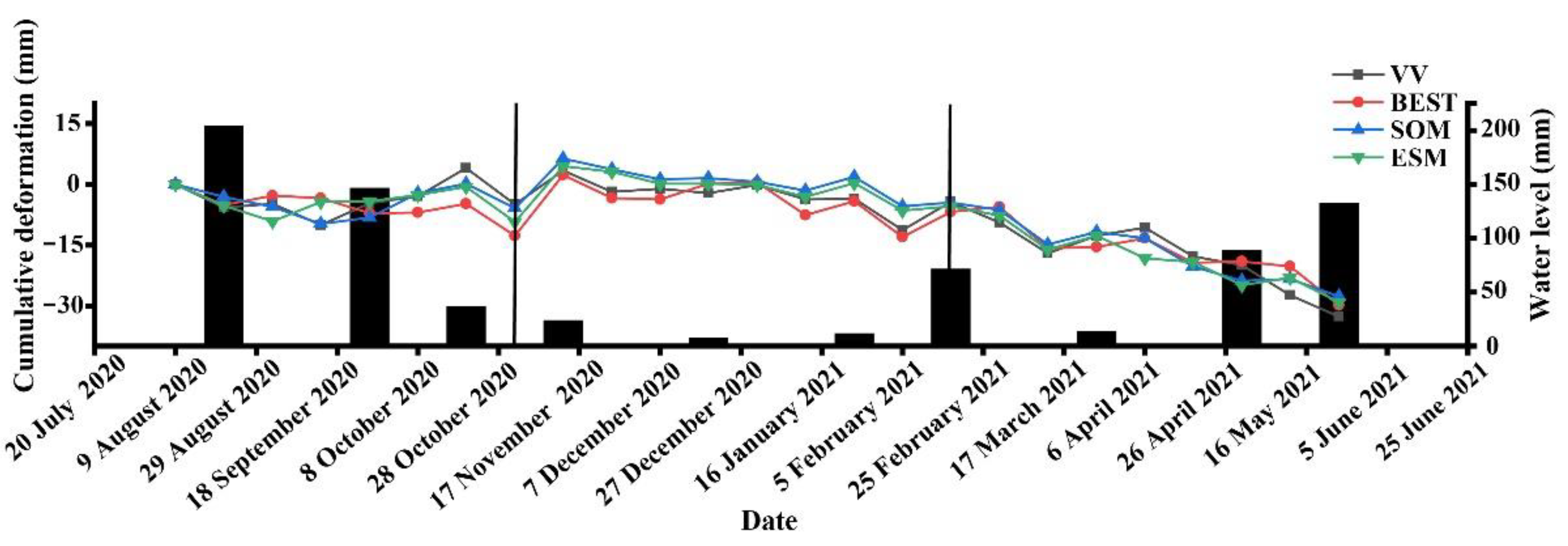
To analyze the accumulated deformation of the tailings reservoir, monitoring points with large accumulated deformation at the same location on the tailings reservoir were selected to examine changes in deformation with time (Figure 12). Changes in accumulated deformation with different methods were similar and consistent. To analyze causes of deformation in the tailings reservoir, local precipitation data were correlated with accumulated deformation (Figure 12). On the basis of experimental results, the deformation of the tailings reservoir was divided into three stages in the study period. The first stage was a settlement stage from 9 August 2020 to 1 November 2020, followed by a slight uplift stage from 1 November 2020 to 17 February 2021, and then a continuous settlement stage from 17 February 2021 to 24 May 2021. From 9 August 2020 to 2 September 2020, because of a large amount of precipitation, the dam body of the tailings reservoir was washed by rainwater, resulting in settlement of the tailings reservoir. Later, also because of a large amount of precipitation, rainwater was recharged, the groundwater level rose, and surface water absorption and expansion led to a slight rise in the tailings reservoir from 2 September 2020 to 20 October 2020. Subsequently, the ponding in the tailings reservoir was discharged through the drainage system, and as a result, the tailings reservoir settled from 20 October 2020 to 1 November 2020. However, from 1 November 2020 to 17 February 2021, when local precipitation decreased significantly and the ground rebounded, the tailings reservoir was less affected by external factors and rose to a certain extent. By contrast, from 17 February 2021 to 24 May 2021, the tailings reservoir continued to settle because of the effect of precipitation.
According to relevant data [23], the deformation of a tailings reservoir is coarse in front of the dam and fine in the pond in the horizontal direction, and there is a serious phenomenon of a fine particle accumulation layer, a cross-layer, and interbedding. In the vertical direction, there is a relation between upper coarse and lower fine, and there are many fan-shaped “sugar core” weak intercalations, showing heterogeneity and anisotropy. In a leaching experiment, first, the tailings swell and rebound. After leaching is stopped for a period of time, the deformation shrinks rapidly and becomes stable. With an increase in leaching time, the deformation gradually tends to zero. Because there are many “sugar core” weak intercalations in tailings reservoirs, monitoring the deformation is essential.
5.2. Calculation Efficiency Analysis
This experiment was conducted on a processor configured with a 5-core Intel (TM) i5-10500 CPU and a 20 GB of RAM computer. The software used was Matlab R2019a. The search step was set to 5°, the experiment was not conducted in parallel, and the GPU was called for processing.
Time required and improvement effect of the three polarization optimization methods were compared (Table 2). The BEST method required the least time, but its improvement effect was not significant. The ESM method required the longest time, but it increased the density of monitoring points in the entire area by 476% and in the tailings reservoir area by 104%. Thus, the optimization effect of the ESM method was substantial. Because the search space of the SOM method was a subspace of the ESM method, its calculation time was shortened by nine hours compared with that with the ESM method. The improvement effect of the SOM method was better than that of the BEST method but inferior to that of the ESM method.
The experimental results showed that additional time was needed to obtain good monitoring results, and as a result, the time spent in optimization could seriously limit the application of this technology in actual production and monitoring. Therefore, to solve this problem, the following aspects can be improved. First, increase the search step of SOM and ESM methods to improve the calculation efficiency and shorten the required time, although this step will inevitably lead to a decline in monitoring results. Second, upgrade computer hardware, configure a higher performance processor, and then parallel the SOM and ESM methods in Matlab and call the GPU for processing, which will help improve the computing efficiency and ensure good monitoring results under the condition that the search step size remains unchanged. Last, use more efficient polarization optimization methods, such as the coherency matrix decomposition (CMD) method [39].
6. Conclusions
In this paper, dual-polarization Sentinel-1 data from 9 August 2020 to 24 May 2021 were acquired. The HTCI algorithm was used to identify the homogeneous points of different polarization channels and fuse them. Pixels were divided into PS and DS pixels, and then three polarization optimization methods (BEST, SOM, and ESM) were used to monitor the deformation of the Kafang tailings reservoir in Gejiu City, Yunnan Province, China. The conclusions were as follows:
- (1)
- Fusing the homogenous points obtained from different polarization channels increased the density of homogenous points, with densities 3.86% and 8.45% higher than that of VH and VV, respectively. The BEST, SOM, and ESM methods were used for polarization optimization. Comparing amplitude dispersion and coherence, the three methods provided significant improvements compared with VV polarization, but the optimization effect was in the order ESM > SOM > BEST.
- (2)
- Deformation monitoring of a tailings reservoir showed that compared with VV polarization, the three optimization methods significantly improved the point selection density. In the image coverage area, the three optimization methods increased the density by 1.83 (BEST), 3.66 (SOM), and 5.76 (ESM) times compared with that with VV polarization, whereas in the tailings reservoir area, density increased by 1.17 (BEST), 1.84 (SOM), and 2.04 (ESM) times.
- (3)
- Correlation coefficients between VV and BEST, BEST and SOM, and SOM and ESM were 0.81, 0.87, and 0.89, respectively, indicating that the calculated deformation rates of the tailings reservoir had a certain reliability. In addition, with the increase in point selection density, SOM and ESM methods effectively reduced the standard deviation of deformation rate, which improved the accuracy of subsequent phase unwrapping.
- (4)
- Although the BEST method increased the point selection density, it only selected the optimal phase on the basis of existing polarization channel data and did not fully use the polarization information. By contrast, the SOM and ESM methods more fully used polarization information to improve the phase quality of pixels by searching the polarization space. However, those two methods needed to use an exhaustive method to search the polarization space, and as a result, the computational efficiency was low. By increasing the step length of the ESPO method, the search times of the whole polarization space will be reduced, and the computational efficiency will be effectively improved, but this means that the monitoring density will decrease. In addition, using parallel computing, calling GPU, or using more efficient CMD methods will effectively solve the problem of low computational efficiency. Therefore, how to improve the computational efficiency of SOM and ESM will be the focus of future research.
Author Contributions
Conceptualization, H.W. and H.F.; methodology, H.W. and X.Z.; software, H.W. and Z.T.; validation, H.W., X.Z. and H.F.; investigation, H.F.; resources, H.F.; writing—original draft preparation, H.W. and H.F.; writing—review and editing, H.W. and H.F.; supervision, H.F.; project administration, H.F.; All authors have read and agreed to the published version of the manuscript.
Funding
This work was supported by the Fundamental Research Funds for the Central Universities under Grant No. 2019XKQYMS23.
Data Availability Statement
Data sharing not applicable.
Acknowledgments
The authors thank the European Space Agency for providing Sentinel-1 data at https://search.asf.alaska.edu/ (accessed on 5 April 2022) and also Jiang Mi for providing the HTCI toolbox.
Conflicts of Interest
The authors declare no conflict of interest.
References
- Adiansyah, J.S.; Rosano, M.; Vink, S.; Keir, G. A framework for a sustainable approach to mine tailings management: Disposal strategies. J. Clean. Prod. 2015, 108, 1050–1062. [Google Scholar] [CrossRef] [Green Version]
- Naeini, M.; Akhtarpour, A. A numerical investigation on hydro-mechanical behaviour of a high centreline tailings dam. S. Afr. Inst. Civil Eng. 2018, 60, 49–60. [Google Scholar] [CrossRef] [Green Version]
- Shan, C.C.; Zhang, Z.D.; Zhong, K.B.; Shi, G.L. Review and summary of handling process of Xiangfen ‘9.8′ extremely major tailings dam break. China Emerg. Manag. 2011, 10, 13–18. [Google Scholar]
- Wu, L.G. Study on Overtopping Dam Failure Mechanism and Protection Measures of Tailings Reservoir. Master’s Thesis, Nanchang University, Nanchang, China, 2021. [Google Scholar]
- Du, Z.Y.; Ge, L.L.; Ng, A.H.M.; Zhu, Q.G.Z.; Horgan, F.G.; Zhang, Q. Risk assessment for tailings dams in Brumadinho of Brazil using InSAR time series approach. Sci. Total Environ. 2020, 717, 137125. [Google Scholar] [CrossRef]
- Ferretti, A.; Prati, C.; Rocca, F. Permanent scatterers in SAR interferometry. IEEE Trans. Geosci. Remote Sens. 2001, 39, 8–20. [Google Scholar] [CrossRef]
- Berardino, P.; Fornaro, G.; Lanari, R.; Sansosti, E. A new algorithm for surface deformation monitoring based on small baseline differential SAR interferograms. IEEE Trans. Geosci. Remote Sens. 2002, 40, 2375–2383. [Google Scholar] [CrossRef] [Green Version]
- Fan, H.D.; Xu, Q.; Hu, Z.; Du, S. Using temporarily coherent point interferometric synthetic aperture radar for land subsidence monitoring in a mining region of western China. J. Appl. Remote Sens. 2017, 11, 026003. [Google Scholar] [CrossRef]
- Iannacone, J.P.; Lato, M.; Troncoso, J.; Perissin, D. InSAR monitoring of active, inactive and abandoned tailings facilities. In Proceedings of the 5th International Seminar on Tailings Management, Santiago, Chile, 11 July 2018; pp. 11–13. [Google Scholar]
- Gamaf, F.; Mura, J.C.; Paradella, W.R.; De Oliveira, C.G. Deformations prior to the Brumadinho dam collapse revealed by Sentinel-1 InSAR data using SBAS and PSI techniques. Remote Sens. 2020, 12, 3664. [Google Scholar] [CrossRef]
- Mazzanti, P.; Antonielli, B.; Sciortino, A.; Scancella, S.; Bozzano, F. Tracking deformation processes at the Legnica Glogow Copper district (Poland) by Satellite InSAR—II: Żelazny Most Tailings Dam. Land 2021, 10, 654. [Google Scholar] [CrossRef]
- Fan, H.D.; Liu, Y.F.; Xu, Y.Z.; Yang, H.L. Surface subsidence monitoring with an improved distributed scatterer interferometric SAR time series method in a filling mining area. Geocarto Int. 2021, 1–23. [Google Scholar] [CrossRef]
- Navarro, V.D.; Lopez, J.M.; Vicente, F. A contribution of polarimetry to satellite differential SAR interferometry: Increasing the number of pixel candidates. IEEE Geosci. Remote Sens. Lett. 2010, 7, 276–280. [Google Scholar] [CrossRef]
- Iglésias, R.; Monells, D.; Fàbregas, X.; Mallorqui, J.J.; Aguasca, A.; Lopez-Martinez, C. Phase quality optimization in polarimetric differential SAR interferometry. IEEE Trans. Geosci. Remote Sens. 2014, 52, 2875–2888. [Google Scholar] [CrossRef]
- Sadeghi, Z.; Zoej, M.J.V.; Hooper, A.; Lopez-Sanchez, J.M. A new polarimetric persistent scatterer interferometry method using temporal coherence optimization. IEEE Trans. Geosci. Remote Sens. 2018, 56, 6547–6555. [Google Scholar] [CrossRef]
- Mullissa, A.; Perissin, D.; Tolpekin, V.; Stein, A. Polarimetry-based distributed scatterer processing method for PSI applications. IEEE Trans. Geosci. Remote Sens. 2018, 56, 3371–3382. [Google Scholar] [CrossRef]
- Zhao, F.; Wang, T.; Zhang, L.X.; Feng, H.; Yan, S.Y.; Fan, H.D.; Xu, D.B.; Wang, Y.J. Polarimetric persistent scatterer interferometry for ground deformation monitoring with VV-VH Sentinel-1 data. Remote Sens. 2022, 14, 309. [Google Scholar] [CrossRef]
- Pan, H.J.; Cheng, Z.Z.; Yang, R.; Zhou, G.H. Geochemical survery and assessment of tailings of the Gejiu tin-polymetallic mining area, Yunnan Province. Chin. J. Geol. Hazard Control. 2015, 42, 1137–1150. [Google Scholar]
- Mao, J.W.; Zhou, Z.H.; Feng, C.Y.; Wang, Y.T.; Zhang, C.G.; Peng, H.J.; Yu, M. A preliminary study of the Triassic large-scale mineralization in China and its geodynamic setting. Geol. China 2012, 39, 1437–1471. [Google Scholar]
- Chen, Y.N.; Li, S.M.; Guo, R.; Yuan, L.W. Study on deformation evolution of sand-covered tailings dam based on time series InSAR. J. Saf. Sci. Technol. 2020, 16, 31–37. [Google Scholar]
- Zhou, M.C.; Chen, Y.H.; Ou, M.X.; Dai, Z.F.; Wang, X.F. Experimental analysis of leaching consolidation on tailings sand. Chin. J. Geol. Hazard Control. 2020, 31, 134–140. [Google Scholar]
- Peng, P.Y.; Wang, W.H. Effect of heavy metal compounds on the micro-aggregate stability in Kafang tailing pond. Agric. Res. Arid. Areas 2020, 38, 215–220. [Google Scholar]
- Wang, X.F. Sedimentary Consoildation Characteristices of Tailings in Kafang Tailings Reservoir and Stability of Tailings Dam. Master’s Thesis, Kunming University of Science and Technology, Kunming, China, 2019. [Google Scholar]
- Jiang, M.; Ding, X.L.; Hanssen, R.F.; Malhotra, R.; Chang, L. Fast statistically homogeneous pixel selection for covariance matrix estimation for multitemporal InSAR. IEEE Trans. Geosci. Remote Sens. 2014, 53, 1213–1224. [Google Scholar] [CrossRef]
- Jiang, M.; Yong, B.; Tian, X.; Malhotra, R.; Hu, R.; Li, Z.W.; Yu, Z.B.; Zhang, X.X. The potential of more accurate InSAR covariance matrix estimation for land cover mapping. ISPRS J. Photogramm. Remote Sens. 2017, 126, 120–128. [Google Scholar] [CrossRef]
- Jiang, M.; Andrea, M.G. Distributed scatterer interferometry with the refinement of spatiotemporal coherence. IEEE Trans. Geosci. Remote Sens. 2020, 58, 3977–3987. [Google Scholar] [CrossRef]
- Kostinski, A.; Boerner, W. On foundations of radar polarimetry. IEEE Trans. Antennas Propag. 1986, 34, 1395–1404. [Google Scholar] [CrossRef]
- Lee, J.S.; Pottier, E. Polarimetric Radar Imaging: From Basics to Applications; CRC: Boca Raton, FL, USA, 2009; pp. 1–398. [Google Scholar]
- Cloude, S.R. Polarisation: Applications in Remote Sensing; Oxford University: New York, NY, USA, 2009. [Google Scholar]
- Cloude, S.R.; Papathanassiou, K.P. Polarimetric SAR interferometry. IEEE Trans. Geosci. Remote Sens. 1998, 36, 1551–1565. [Google Scholar] [CrossRef]
- Cloude, S.R. Wideband radar inversion studies using the entropy-alpha decomposition. Proc. SPIE Int. Soc. Opt. Eng. 1997, 37, 2430–2441. [Google Scholar]
- Chen, S.W.; Wang, X.S.; Sato, M. PolInSAR complex coherence estimation based on covariance matrix similarity test. IEEE Trans. Geosci. Remote Sens. 2012, 50, 4699–4710. [Google Scholar] [CrossRef]
- Pipia, L.; Fabregas, X.; Aguasca, A.; Lopez-Martinez, C.; Duque, S.; Mallorqui, J.J.; Marturia, J. Polarimetric differential SAR interferometry: First results with ground-based measurements. IEEE Geosci. Remote Sens. Lett. 2009, 16, 167–171. [Google Scholar] [CrossRef]
- Neumann, M.; Ferro-Famil, L.; Reigber, A. Multibaseline polarimetric SAR interferometry coherence optimization. IEEE Geosci. Remote Sens. Lett. 2008, 5, 93–97. [Google Scholar] [CrossRef] [Green Version]
- Azadnejad, S.; Maghsoudi, Y.; Perissin, D. Evaluation of polarimetric capabilities of dual polarized Sentinel-1 and TerraSAR-X data to improve the PSInSAR algorithm using amplitude dispersion index optimization. Int. J. Appl. Earth Obs. Geoinf. 2020, 2, 101950. [Google Scholar] [CrossRef]
- Sagues, L.; Lopez-Sanchez, J.; Fortuny, J.; Fabregas, X.; Broquetas, A.; Sieber, A.J. Indoor experiments on polarimetric SAR interferometry. IEEE Trans. Geosci. Remote Sens. 2000, 38, 671–684. [Google Scholar] [CrossRef]
- Ferretti, A.; Fumagalli, A.; Novali, F.; Prati, C.; Rocca, F.; Rucci, A. A new algorithm for processinginterferometric data-stacks SqueeSAR. IEEE Trans. Geosci. Remote Sens. 2011, 49, 3460–3470. [Google Scholar] [CrossRef]
- Efron, B. Bootstrap methods: Another look at the jackknife. Ann. Stat. 1979, 7, 1–26. [Google Scholar] [CrossRef]
- Zhao, F.; Jordi, J.J. Coherency matrix decomposition-based polarimetric persistent scatterer interferometry. IEEE Trans. Geosci. Remote Sens. 2019, 57, 7819–7831. [Google Scholar] [CrossRef] [Green Version]
Figure 1.
Location of the study area: (a) map of Yunnan, China; (b) location of the study area in Yunnan Province; (c) satellite image of the study area and tailings reservoir.
Figure 1.
Location of the study area: (a) map of Yunnan, China; (b) location of the study area in Yunnan Province; (c) satellite image of the study area and tailings reservoir.
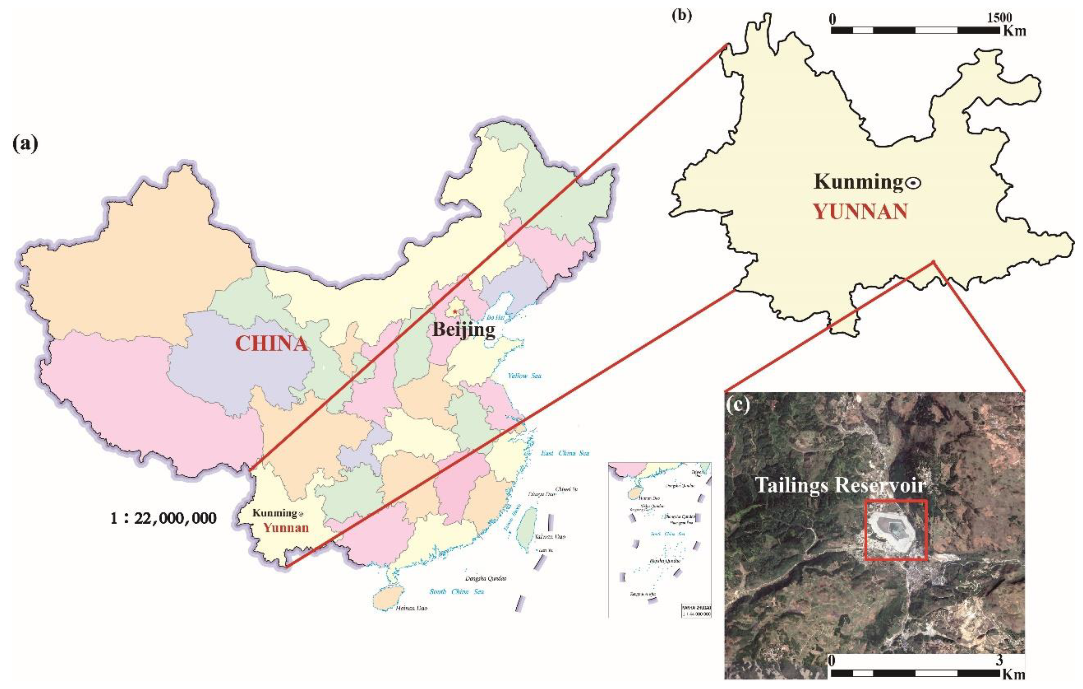
Figure 2.
Flowchart of data processing.

Figure 3.
Temporal and perpendicular baseline graph of the generated interferogram stack. Red and green dots represent primary and secondary SAR images forming the interferograms, respectively.
Figure 3.
Temporal and perpendicular baseline graph of the generated interferogram stack. Red and green dots represent primary and secondary SAR images forming the interferograms, respectively.
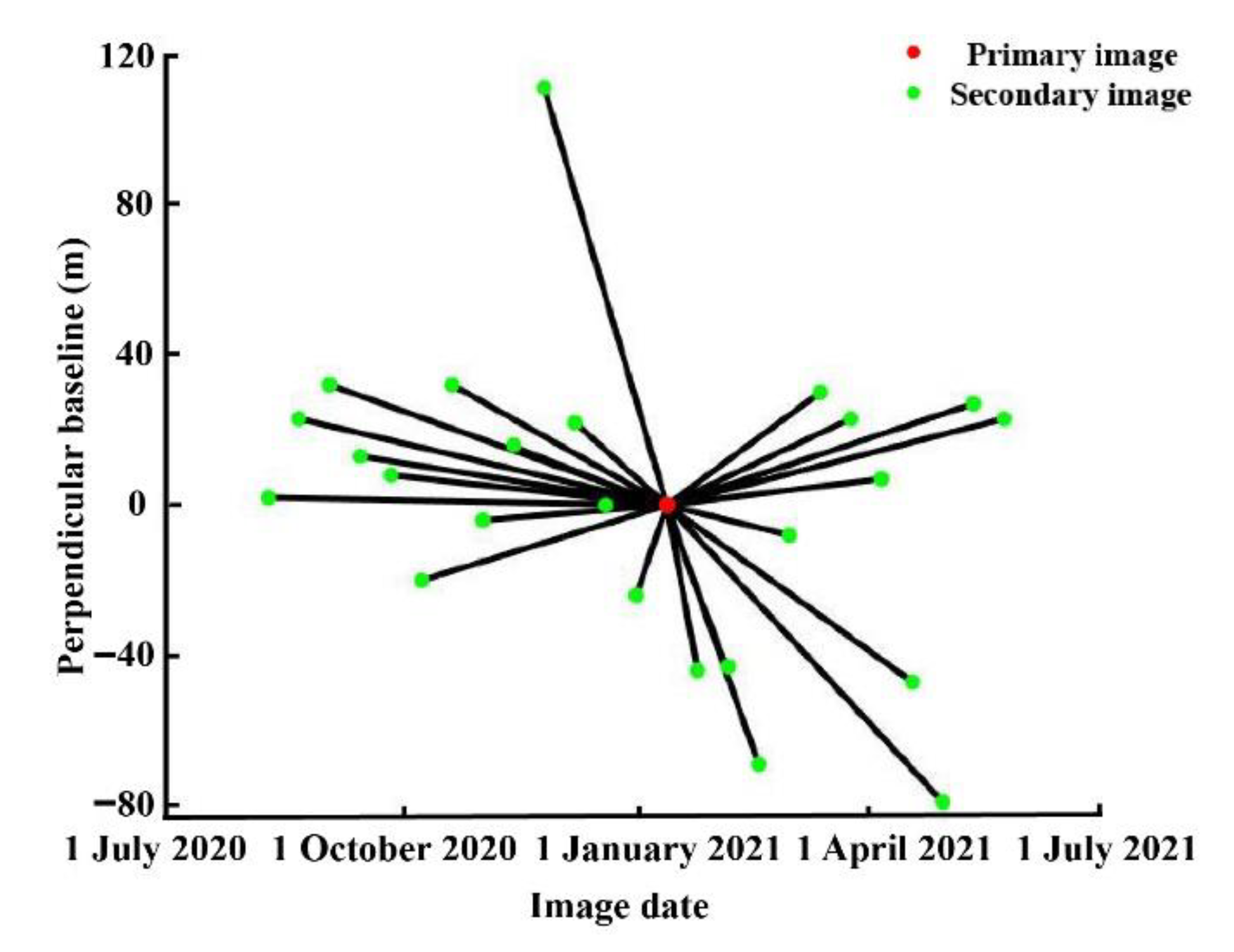
Figure 4.
Number of homogeneous pixels selected by different polarimetric channels: (a) VV polarimetric; (b) VH polarimetric; and (c) VV + VH polarimetric channels. Red rectangles A, B, and C represent the selected special area, respectively. The chromaticity bar on the right indicates the number of selected homogeneous points.
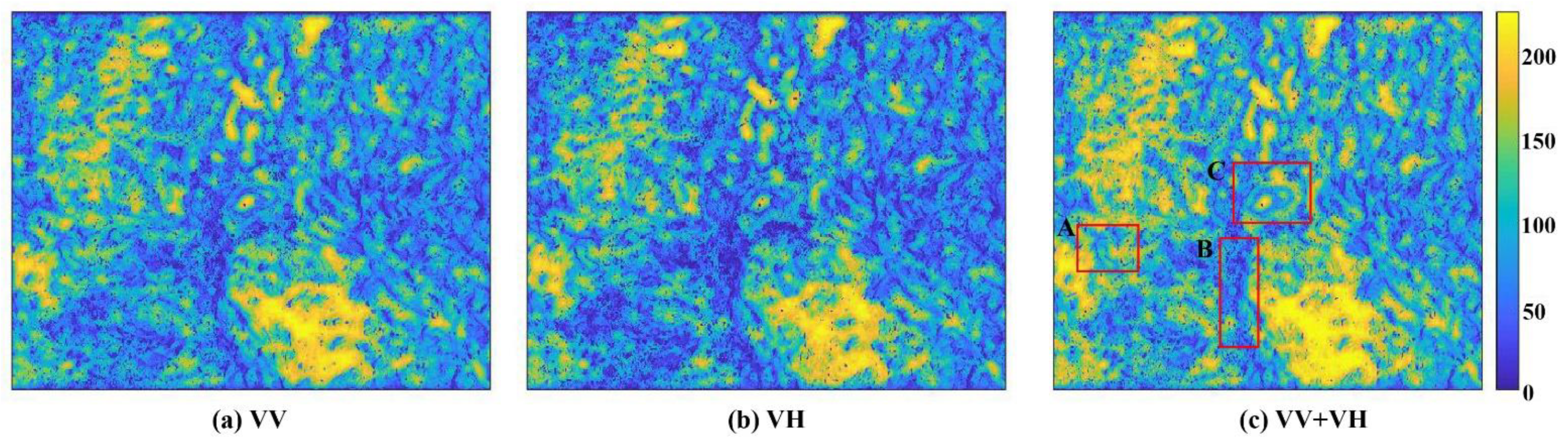
Figure 5.
Schematic diagram of homogeneous point recognition of different targets. Red is the reference point, and green is the identified homogeneous point. In the left figure, (a), (b), and (c) represent the selected feature points, respectively.
Figure 5.
Schematic diagram of homogeneous point recognition of different targets. Red is the reference point, and green is the identified homogeneous point. In the left figure, (a), (b), and (c) represent the selected feature points, respectively.
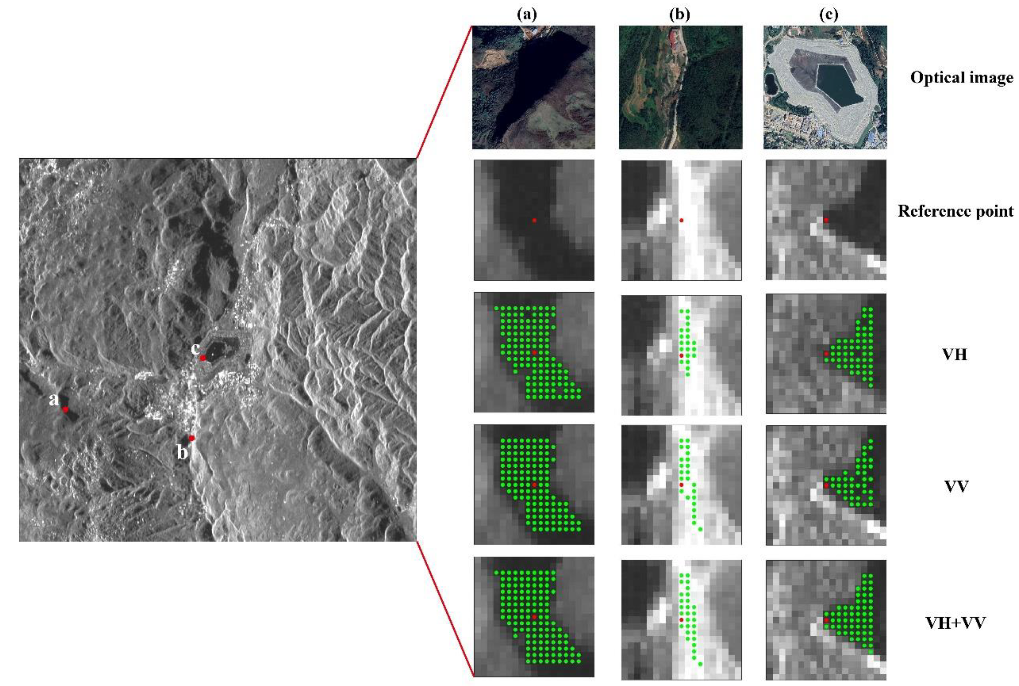
Figure 6.
(a) Amplitude dispersion index () histograms, with (b) a detailed zoom of the black rectangle in (a).
Figure 6.
(a) Amplitude dispersion index () histograms, with (b) a detailed zoom of the black rectangle in (a).
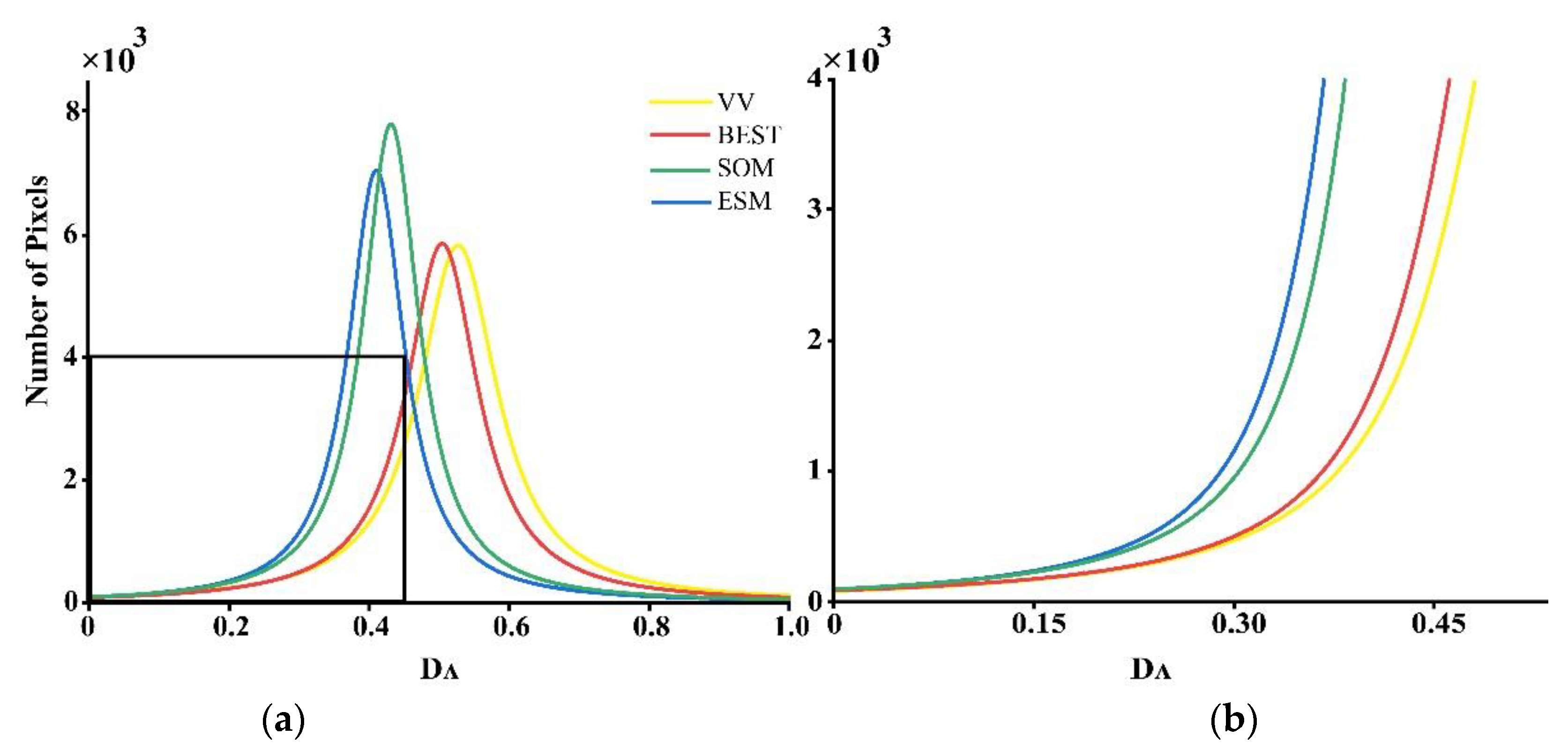
Figure 7.
(a) Mean coherence index () histograms, with (b) a detailed zoom of the black rectangle in (a).
Figure 7.
(a) Mean coherence index () histograms, with (b) a detailed zoom of the black rectangle in (a).
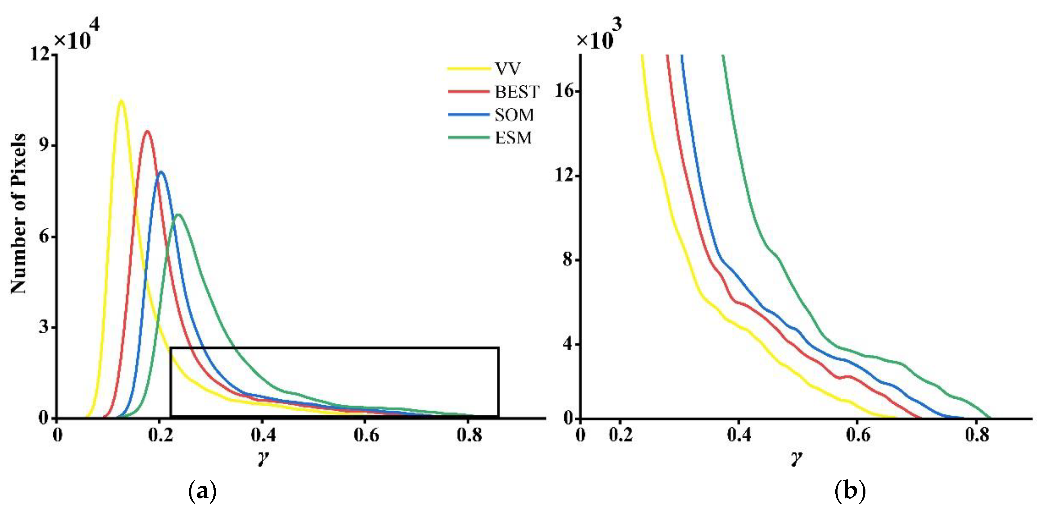
Figure 8.
Monitoring results of deformation rate of a tailings reservoir: (a), (b), (c), and (d) represent deformation rate results of VV, BEST, SOM, and ESM methods, respectively; (e), (f), (g), and (h) represent deformation rate results of VV, BEST, SOM, and ESM methods in red rectangular areas. The number and () in the upper left corner indicate the number of highly coherent points selected and percentage increase by different methods w.r.t that of the VV channel.
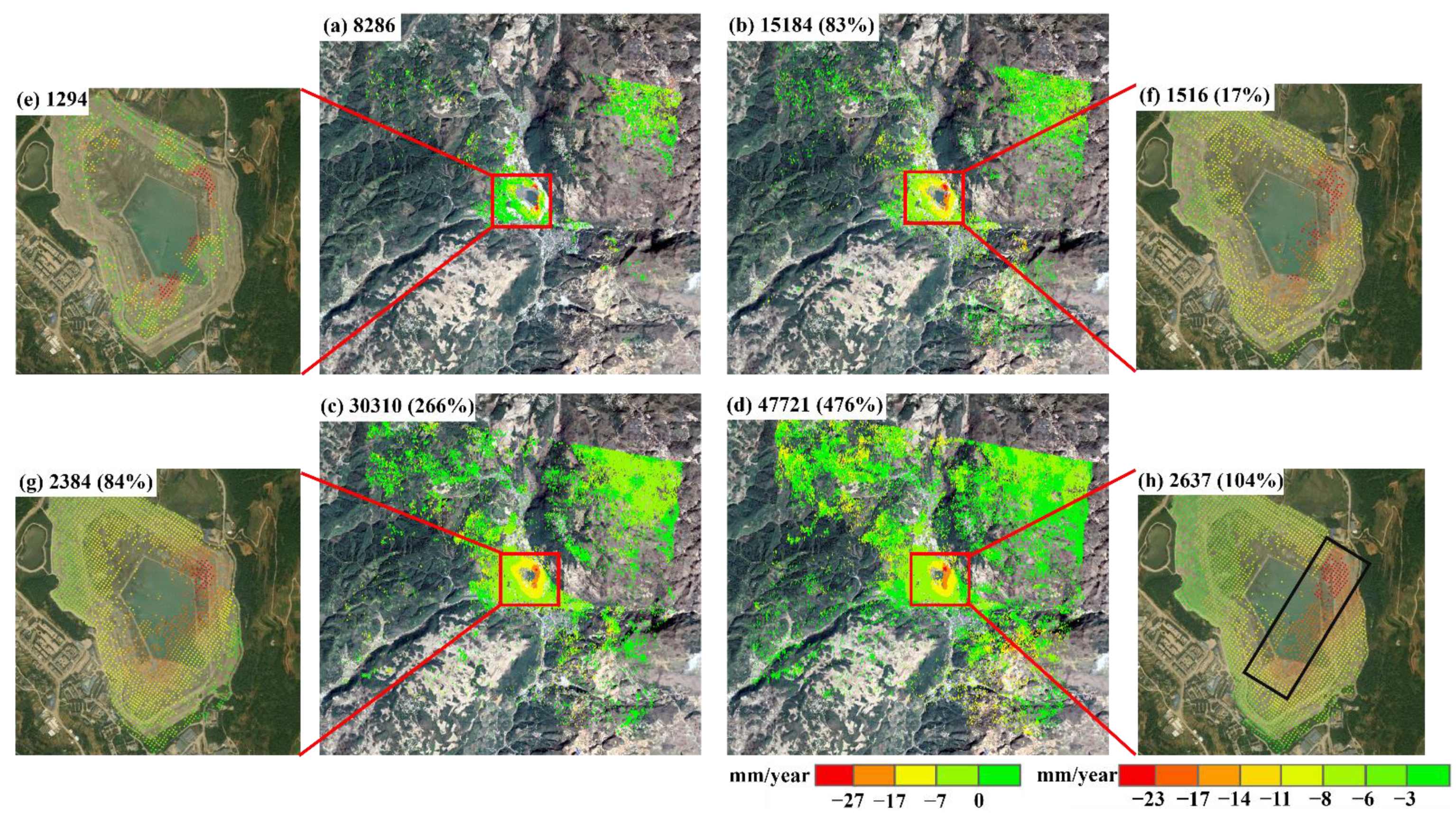
Figure 9.
The scatter diagram of completely coincident points deformation rates for: (a) VV–BEST; (b) BEST–SOM; and (c) SOM–ESM methods.
Figure 9.
The scatter diagram of completely coincident points deformation rates for: (a) VV–BEST; (b) BEST–SOM; and (c) SOM–ESM methods.
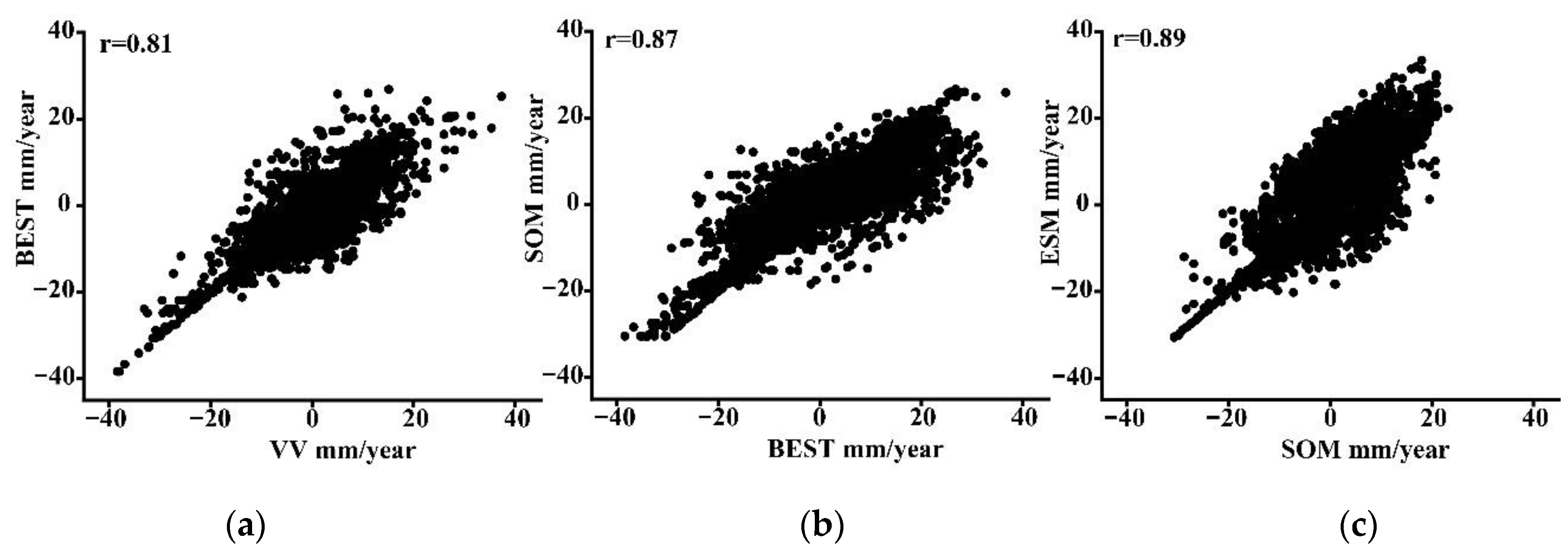
Figure 10.
Histograms of standard deviation of deformation rate derived from: (a) VV; (b) BEST; (c) SOM; and (d) ESM methods.
Figure 10.
Histograms of standard deviation of deformation rate derived from: (a) VV; (b) BEST; (c) SOM; and (d) ESM methods.
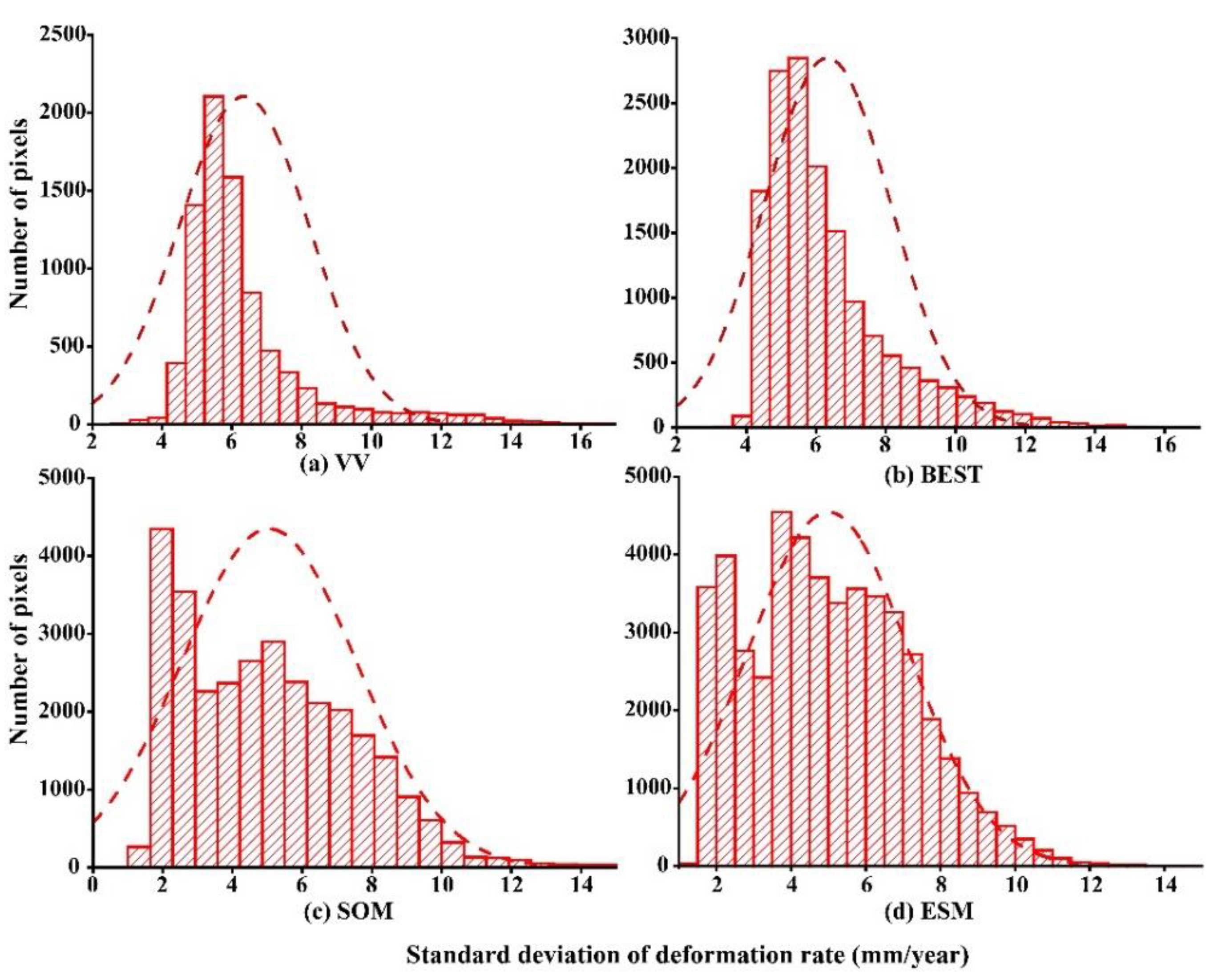
Figure 11.
Profiles of deformation rate of a tailings reservoir. Transects: (a) A–A′; (b) B–B′; and (c) C–C′.
Figure 11.
Profiles of deformation rate of a tailings reservoir. Transects: (a) A–A′; (b) B–B′; and (c) C–C′.
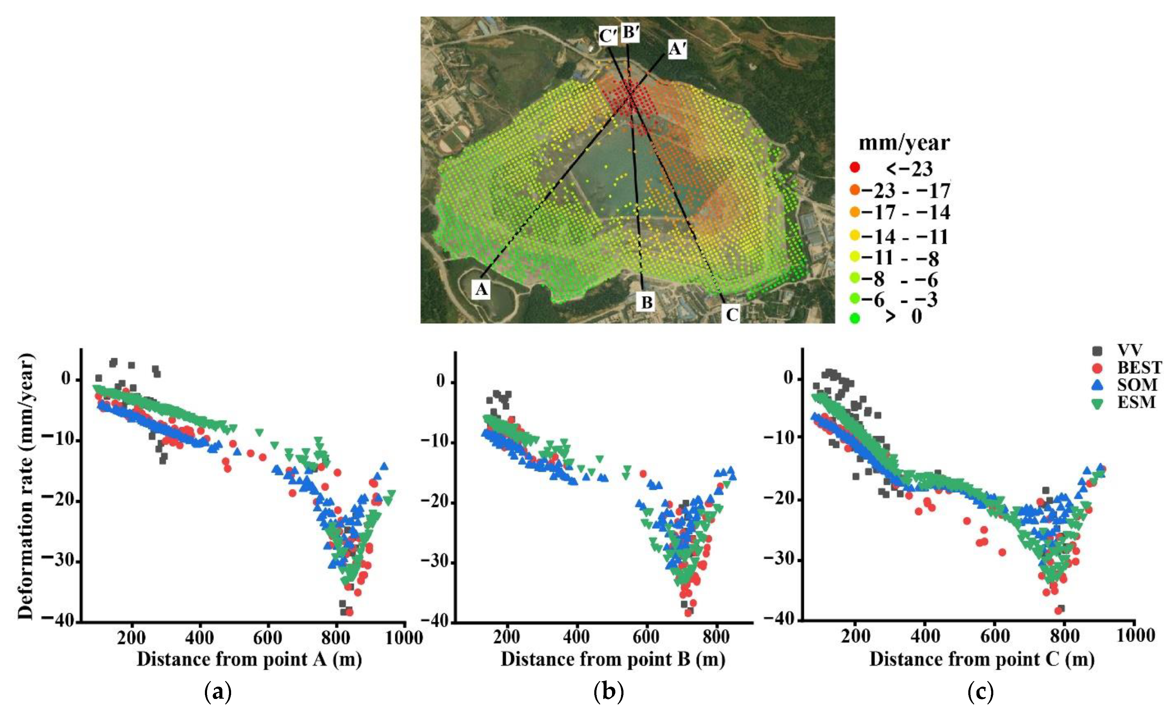
Figure 12.
Correlation diagram between time series deformation and precipitation of monitoring points at the same location.
Figure 12.
Correlation diagram between time series deformation and precipitation of monitoring points at the same location.

Table 1.
Comparison of SHP recognition results.
| Polarization | Mean Value | SHP > 20 | Improvement (%) |
|---|---|---|---|
| VH | 74 | 225,142 | 3.86 |
| VV | 68 | 215,618 | 8.45 |
| VH + VV | 89 | 233,831 |
SHP represents statistically homogeneous pixel. Polarization and Improvement represent different polarization channels and the percentage of increase of VH + VV compared with SHP of single polarization channels, respectively.
Table 2.
Polarimetric optimization computation time of PolPSI techniques.
| Method | Time (h) | Improvement | Test Site |
|---|---|---|---|
| BEST | 1.5 | 83% (17%) | Kafang (500 × 2500) |
| SOM | 28 | 266% (84%) | |
| ESM | 37 | 476% (104%) |
Method represents the polarization optimization method used. Time represents the time required for different methods. Improvement, and () represent the percentage of increase in high coherence points in the whole study area and the tailings reservoir area w.r.t. that of VV channel, respectively. Test site represents the study area, and () represent the size of the image.
Publisher’s Note: MDPI stays neutral with regard to jurisdictional claims in published maps and institutional affiliations. |
© 2022 by the authors. Licensee MDPI, Basel, Switzerland. This article is an open access article distributed under the terms and conditions of the Creative Commons Attribution (CC BY) license (https://creativecommons.org/licenses/by/4.0/).
Share and Cite
MDPI and ACS Style
Wu, H.; Zheng, X.; Fan, H.; Tian, Z. Deformation Monitoring of Tailings Reservoir Based on Polarimetric Time Series InSAR: Example of Kafang Tailings Reservoir, China. Remote Sens. 2022, 14, 3655. https://doi.org/10.3390/rs14153655
AMA Style
Wu H, Zheng X, Fan H, Tian Z. Deformation Monitoring of Tailings Reservoir Based on Polarimetric Time Series InSAR: Example of Kafang Tailings Reservoir, China. Remote Sensing. 2022; 14(15):3655. https://doi.org/10.3390/rs14153655
Chicago/Turabian StyleWu, Hao, Xiangyuan Zheng, Hongdong Fan, and Zeming Tian. 2022. "Deformation Monitoring of Tailings Reservoir Based on Polarimetric Time Series InSAR: Example of Kafang Tailings Reservoir, China" Remote Sensing 14, no. 15: 3655. https://doi.org/10.3390/rs14153655
Note that from the first issue of 2016, this journal uses article numbers instead of page numbers. See further details here.