
Nightlight Intensity Change Surrounding Nature Reserves: A Case Study in Orbroicher Bruch Nature Reserve, Germany


1
Applied Analysis Solutions, 535 McDonald Rd, Winchester, VA 22602, USA
2
Bayer AG, Alfred-Nobel-Str. 50, 40789 Monheim, Germany
*
Author to whom correspondence should be addressed.
Remote Sens. 2022, 14(16), 3876; https://doi.org/10.3390/rs14163876
Submission received: 8 June 2022
/
Revised: 20 July 2022
/
Accepted: 29 July 2022
/
Published: 10 August 2022
(This article belongs to the Special Issue Remote Sensing of Night-Time Light)
Abstract
:Persistent global urbanization has a direct relationship to measurable artificial light at night (ALAN), and the Defense Meteorological Satellite Program has served an important role in monitoring this relationship over time. Recent studies have observed significant declines in insect abundance and populations, and ALAN has been recognized as a contributing factor. We investigated changes in nightlight intensity at various spatial scales surrounding insect traps located in Orbroicher Bruch Nature Reserve, Germany. Using a time series of global nighttime light imagery (1992–2010), we evaluated pixel-level trends through linear regressions and the Mann–Kendall test. Paired with urban land cover delineation, we compared nightlight trends across rural and urban areas. We utilized high-resolution satellite imagery to identify landscape features potentially related to pixel-level trends within areas containing notable change. Approximately 96% of the pixel-level trends had a positive slope, and 22% of pixels experienced statistically significant increases in nightlight intensity. We observed that 80% of the region experienced nightlight intensity increases >1%, concurrent with the observed decline in insect biomass. While it is unclear if these trends extend to other geographic regions, our results highlight the need for future studies to concurrently investigate long-term trends in ALAN and insect population decline across multiple scales, and consider the spatial and temporal overlaps between these patterns.
1. Introduction
A decline in insect abundance and populations has been observed across many regions in recent decades [1,2]. Previous studies measuring insect biomass through insect traps have found significant declines in biomass through long-term, multiyear observations [2,3,4]. Owens et al. [1] suggest that the combination of climate change, habitat loss, chemical pollutants, invasive species, and artificial light at night (ALAN) are key factors driving insect decline. Approximately 30% of vertebrates and 60% of invertebrates across the world are nocturnal [5]. Light is an important factor for many key behavioral and biological processes of insects. They rely on nocturnal light for navigation, avoiding predation, foraging, reproduction, and regulating their biological clocks [1,2], and ALAN has been observed to affect these biological processes (Owens et al., 2020). ALAN has been identified as a factor directly contributing to declines in moth populations and other insects with strong phototactic responses [5,6]. Additionally, ALAN has been observed to influence the community composition of aquatic primary producers [2].
The increases in ALAN have been primarily attributed to human settlements and the process of urbanization. ALAN is widespread and has been increasing over the last decades worldwide at an annual rate of 2–6%, imposing an unprecedented alteration of natural light regimes [2,5]. The impacts of ALAN are not limited to the immediate surroundings of the light source. More remote areas can be affected by light pollution [1,2] through skyglow [7,8], which can reach dozens of kilometers beyond the original source [9,10] and the effects are amplified by overcast skies [11]; therefore, even nature reserves and other protected areas are not always shielded from ALAN pollution [12]. Given the average increasing rate of ALAN worldwide, the effects of ALAN on declining insect populations should be further investigated at local and regional spatial scales [7].
The Defense Meteorological Satellite Program Operational Linescan System (DMSP-OLS) satellites detect low levels of electromagnetic radiation emitted at night at wavelengths within the visible and near-infrared (VNIR) portion of the electromagnetic spectrum, spanning 0.5 nm–0.9 nm [13,14,15]. Documented sources of nightlight emission include city lights, gas flares, and wildfires [13,14,15]. Previous studies have found that nightlight imagery can be used to map urban areas since spatiotemporal patterns in nightlight intensity correspond to patterns in modern human settlements [13,15,16]. Artificial lights at night have also been used to develop indicators of economic productivity [17]. In Europe, trends in ALAN over time captured by DMSP-OLS satellites have been related to specific landscape changes [18]; increases in ALAN have generally been attributed to suburban and industrial development, and decreases related to energy efficiency improvements and periods of economic decline [18].
Increases in ALAN at different scales can impact trophic interactions [19], ecological functions [2,20], and alter biodiversity [20,21]. Some studies have emphasized the need to consider and manage ALAN within protected areas [12,22]. The impacts of ALAN on populations, communities, and ecosystems vary across regions and spatial scales. Previous studies utilizing remotely sensed imagery and landscape ecology concepts have found that ALAN has significantly reduced the areas considered to be suitable habitat (lacking nighttime light pollution) and has negatively impacted biodiversity within natural reserves [12]. ALAN impacting protected nature reserves is a globally observed phenomenon. Fan et al. [23] suggest that biodiversity data should be paired with nightlight satellite imagery to investigate the effects of light pollution and optimize buffer distances surrounding protected areas. The impacts of lighting on ecosystems vary based on the economic and social contexts, suggesting that the optimal buffer distance around protected areas differs for each unique scenario [23,24]. There is not a one-size-fits-all solution for optimizing the configuration of light pollution, anthropogenic structures, and their proximity to nature reserves, presenting the need to consider all relevant factors in landscape planning.
In this study, we investigated changes in nightlight intensity captured by satellite imagery at varying radii (1, 2, and 10 km) surrounding the two insect trap locations in the Orbroicher Bruch Nature Reserve in Germany utilized by Hallmann et al. [4]. First, we tested trends in ALAN between 1992 and 2010, using global nightlight intensity satellite imagery to investigate pixel-level changes using linear regressions and the Mann–Kendall test. Paired with an urban land cover designation from CORINE (2012) and high-resolution satellite imagery, we compared trends of nightlight intensity through time across rural and urban areas. Within areas where we identified significant changes in nightlight intensity, we attributed the specific alterations on the land surface as potential causes or contributing factors to the change using a combination of aerial imagery, historical records, and expert knowledge. By pairing the timeframe of change with specific surface features, we outline a methodology that highlights specific landscape changes to consider as potential contributors to insect decline in future investigations. We present a novel investigation of observed insect decline and nightlight satellite imagery corresponding to the time period and geographic region [4]. These methods have the potential to be further developed and refined to assess the efficacy of nightlight mitigation efforts, identify structures with significant impacts on nightlight pollution, consider the effects of changes from smaller intense light and wider area diffuse light, and further support landscape management decisions in the context of insect conservation.
2. Materials and Methods
2.1. Study Area and Time Period
Within North Rhine-Westfalia, Germany we examined the landscape within a 10 km radius surrounding two insect trap locations (Figure 1) to investigate changes in nightlight intensity between 1992 and 2010. The total area spans roughly 318 km2, and overlaps with 11 municipalities, although the majority of the study area is comprised of Krefeld, Kempen, Rheurdt, Tönisvorst, Kerken, and Neukirchen-Vluyn. The traps are located near Krefeld within Orbroicher Bruch, which is a nature reserve. Nature reserves are a class of protected areas under Germany’s Federal Nature Conservation Act primarily used to facilitate species conservation. Orbroicher Bruch covers roughly 1 km2 of protected forest, wet grasslands, and marshes. The surrounding region is comprised of cropland, forest, grasslands, and urban areas. The population of North Rhine-Westphalia has grown from approximately 17.1 million in 1989 (source) to 17.9 million in 2010 (retrieved from data commons timelines based on Europa.eu, measurement method = Eurostat regional population data). Previous studies using satellite imagery to model land cover have estimated that impervious surfaces from urban development have increased by roughly 30% (1670 km2) between 1985 and 2017 in North Rhine-Westphalia [25].
2.2. Remote Sensing Data (DMSP-OLS Nighttime Lights Time Series)
We gathered a time series of satellite images between 1992 and 2010 of Global Night-Time Light intensity [Version 4] captured by the DMSP-OLS at a 30 arc-second spatial resolution (roughly 1.5 km × 0.9 km at 51.4° N) (Figure 2) (data retrieved from https://ngdc.noaa.gov/eog/dmsp/download V4composites.html, accessed on 20 April 2022). We selected the DMSP-OLS satellite imagery since it provided global data measuring nightlight intensity corresponding to our time period of interest. Images covering the 10 km radius region surrounding the Orbroicher Bruch Nature Reserve were acquired from seven DMSP-OLS satellites (F10, F11, F12, F14, F15, F16, and F18) to capture the full 19-year period. This dataset contains annual, cloud-free composites of light intensity at night and has been processed to remove sunlit images, moonlit images, images containing glare, as well as any light features from the aurora in the Northern hemisphere [15,26]. In years where two annual composites were available because two satellites collected overlapping data, we selected a single composite collected by one satellite for the given year to maintain consistency with the years with only one composite. We selected the stable lights average band within this dataset, which covers cities, towns, and other regions with perpetual light emission; these data are provided in digital numbers and have been filtered for background noise from other sources of VNIR emissions (e.g., gas flares) [15,26]. Since the DMSP-OLS does not have on-board calibration, it is not feasible to compare digital numbers across multiple years without additional processing [27]. Therefore, we performed an intercalibration of DMSP-OLS images using the software GRASS GIS (Version 7.4) based on the coefficients and approach of Wu et al. [27].
2.3. Remote Sensing Trend Analysis
We assessed spatial and temporal trends in nightlight intensity values from the calibrated DMSP-OLS time series at the individual pixel scale to identify significant changes in nightlight intensity over time (Figure 2). To identify trends, we estimated linear regressions on a pixel-level basis and examined the regression slope within each pixel. We selected the Mann–Kendall statistical test for use in this analysis as a non-parametric test for environmental time series data, to measure the direction and strength of monotonic, pixel-level trends. We used R [V 3.4.3] to estimate linear regressions and apply the Mann–Kendall test using the “Kendall” package [V 2.2] [28,29,30,31]. The results from the Mann–Kendall test include Kendall’s tau statistic, which indicates trend strength and direction, as well as a two-sided p-value to determine the statistical significance of the monotonic trends. Kendall’s tau statistic ranges from –1 to 1, where positive or negative values closer to zero are less significant, and values closer to −1 or 1 exhibit stronger trends, with the sign indicating the directionality of the trend.
We applied this methodology to the full time period (1992–2010) as well as the early (1992–1999) and late (2003–2010) time periods we defined to analyze the differences between the beginning and end of the investigation period. For the subset of annual images captured within both the early and late time periods, the median nightlight intensity value was calculated for each pixel. Additionally, we calculated the relative difference between the early and late time periods for each pixel to identify substantial changes in nightlight intensity in areas where values did not fall on the extreme ends of the spectrum. The full time period of interest captured the overall trend, whereas the comparisons between the early and late time periods allowed us to compare regional changes in nightlight intensity.
2.4. Urbanization Analysis
In order to explore potential causes of change in nightlight intensity, we first characterized land use and land cover (LULC) across our study area, since urbanization coincides with increasing nightlight intensity (Figure 2). We utilized the CORINE land cover dataset from 2012 (data retrieved from https://land.copernicus.eu/pan-european/corine-land-cover/clc-2012, accessed on 4 May 2022) to delineate urban and rural areas within the full study area. We selected all areas defined as continuous (1.1.1) and discontinuous urban fabric (1.1.2), construction sites (1.3.3), dump sites (1.3.2), as well as industrial or commercial units (1.2.1) to represent urban land cover. Port areas (1.2.3) and airports (1.2.4) were not present within the study region, while green urban areas (1.4.1) and sport and leisure facilities (1.4.2) were not included in the urban areas we defined since they contain vegetation cover. All areas that did not meet these criteria were classified as rural (i.e., not urban); rural areas included farmland, water, forests, and other land cover classes, although many of these areas may contain sparse or patchy developed areas (human features).
To connect this classification with the nightlights time series imagery, a grid representing the individual pixels of the nightlight’s dataset was intersected with the rural/urban land cover classification, and pixels were designated as urban or rural based on the majority type (≥50% of the given pixel). We summarized the total area of pixels classified as rural and urban across the full study area for 2012. In addition, we compared the pixel-level trends in nightlight intensity (from linear regressions based on the early and late time periods and the Mann-Kendall test across the full study period) between the pixels classified as urban and rural to characterize patterns occurring within these contrasting land cover types.
2.5. Change Attribution
We utilized pixel-level statistics to identify temporal and spatial trends in nightlight intensity indicative of landscape feature changes, and to describe potential agents or features contributing to the pixel-level trend (Figure 2). Within the full time period (1992–2010), we used the Mann–Kendall test to identify pixel-level instances of relative, significant local and regional changes in nightlight intensity within 1, 2, and 10 km radii around the insect trap locations. Within the 1 and 2 km radii, we considered all pixels at each scale, and identified all potentially relevant features that had changed; we chose to examine all surrounding features at these scales due to the effects that direct lighting can have on insect habitats and nature preserves. We also examined the 10 km radius (full study area) to identify regional changes in nightlight intensity; it is important to consider this scale based on the range of insect movement, insect metapopulation dynamics, and because nightlight pollution (indirect effects) can span many kilometers, especially with overcast skies. Within the 10 km radius, we selected two subsets of pixels that met specific criteria to further explore local, feature-based changes. The first group of pixels (ID’s 1–10) had a slope > 0 and R2 > 0.3 based on the linear trend analysis; they also had a relative early to late difference (between 1992–1999 and 2003–2010) > 0 and statistically significant change (α < 0.1). The second group of pixels that was further investigated (ID’s 11–17) had high slope values >0.86. These pixels were not selected based on any level of alpha significance or any particular R2 value.
At each spatial scale considered, we utilized historical aerial imagery to investigate sub-pixel features (Figure 2). Historical imagery collected through the North Rhine-Westphalia aerial photography catalog was provided by the District Government of Cologne, and captured in 1989 (start of the study period) at a 40 × 40 cm spatial resolution and in 2013 (end of the study period) at a 10 × 10 cm spatial resolution. Chronological aerial imagery from Google Earth was also used to supplement the identification of changes that took place during the study period. Features of interest identified via aerial imagery were further verified by incorporating expert knowledge and relevant, supporting documentation (Figure 2). External expert knowledge included a local landscape photographer, Paul Maaßen, and community officials in Krefeld. Identifying specific features that changed based on historical aerial imagery, and supporting these findings with external knowledge and documentation, provided the framework for relating these landscape features to observed trends in nightlight intensity.
While the spatial resolution of the DMSP-OLS time series data is coarser than the landscape features investigated, we also considered that a variety of sub-pixel spatial configurations of landscape features could contribute to the pixel-level trend. For example, a pixel with a one percent increase in nightlight intensity has many potential spatial configurations, as displayed in Figure A1. A single hectare that experienced a 100 percent increase in nightlight intensity, or 20 hectares that experienced a five percent increase in nightlight intensity, are both potential spatial configurations of the generalized pixel-level trend (one percent increase). The variety of sub-pixel spatial configurations responsible for pixel-level trends is an influential factor that was considered throughout the process of evaluating and attributing changes to specific landscape features.
3. Results
3.1. Image (Pre-)Processing
Nightlight intensity values from DMSP-OLS V4 image collections are stored as digital numbers which are the raw values captured at the sensor corresponding to the intensity of reflectance. The original digital numbers range from 1 to 63, from lowest to highest intensity; the stable lights average composites were processed to remove the temporary events causing background noise, and these values were replaced with 0. Areas completely covered by clouds are represented by the value 255. After intercalibration of the images using the invariant region method [27], the digital numbers of the nightlight intensity values are rescaled, as shown in Figure 3 (ranging from 1 to 100+). In both the uncalibrated and calibrated DMSP-OLS time series images, pixel regions with the greatest nightlight intensity (highest values, shown in yellow) generally correspond with urban areas. The areas with the brightest nightlight can be identified in the southeastern portion of the study area in Figure 3b, which geographically corresponds to the areas classified as urban in Figure 1 and Figure 4.
3.2. Nightlight Trend Analysis
3.2.1. Overall Trends
The linear regression estimation and Mann–Kendall test revealed comparable relationships between increasing urbanization and increasing intensity values. Across the full time series (1992–2010, DMSP-OLS), we observed a general increase in nightlight intensity that was more prominent within localized clusters (Figure 5), likely reflecting development and urbanization patterns. Approximately 22% of the region demonstrated statistically significant (α < 0.1) trends in nightlight intensity based on the Mann–Kendall test, and 13.4% of the region had statistically significant trends of increasing or decreasing nightlight intensity over the 19-year period at α < 0.05 (Table A1). Based on the Mann–Kendall tau statistic, many of the statistically significant changes in nightlight intensity were clustered in the northwest of the study area (Figure 5). Decreases in nightlight intensity were only observed in 13 of the 590 (3%) pixels covering the region (also indicated by the Mann–Kendal tau statistic) (Figure 5).
Median nightlight intensity in the early and late time periods are shown in Figure 6 and Figure A2. Between the early and late time periods, the mean pixel-level change in nightlight intensity across the region was an increase of 7%, with a maximum increase of 47% and decrease of −17% (Figure 7). We also evaluated the number of pixels that exceeded varying thresholds (1, 5, 10, and 25%) of nightlight intensity increase between the two time periods. We generally observed that 80% of pixels exceeded the 1% threshold in nightlight intensity between the early and late time periods (Figure 8). A general trend of increasing lighting was observed across the majority of the study area. The pixels that exceeded the 5% and 10% nightlight intensity increase thresholds corresponded with urbanization and varying degrees of new settlement or development (Figure 8). However, only 4% of the study area experienced greater than a 25% increase in nightlight intensity, and this was attributed to intensive land use changes in these areas, with high lighting requirements related to industry and greenhouses (Figure 8). The nightlight intensity thresholds exceeded by a given pixel between the early and late time periods depend on the amount of existing urban development present and the initial observation of intensity in the early time period, implying that change is relative to each pixel (Figure 7). The magnitude of change observed is multifactorial, and we further explored the types of infrastructure and spatial configuration of land use changes corresponding to the observed trends in Section 3.3.
3.2.2. Urban/Rural
Through historical, fine-resolution aerial imagery, we visually identified an increase in urban land cover between 1989 and 2013. Approximately 82% of the region (out of the 590 pixels) was classified as rural, and inversely, 18% of the region was classified as urban in 2012 (Table A2). The predominant categorization across the region (10 km radius) was classified as rural, and overall, we observed a more prominent increase in nightlight intensity within these rural areas compared to urban areas (Figure 9). Most significant changes in nightlight intensity (Mann–Kendall p-values, α < 0.05) were related to increases that occurred within rural areas (Figure 4 and Figure 5). A larger proportion of the study area classified as rural had positive Mann–Kendall tau values and corresponded to statistically significant increases in nightlight intensity (p-values, α < 0.05), while a smaller proportion of urban areas experienced statistically significant increases. Our results from the Mann–Kendall test revealed some pixels with negative tau values, indicating nightlight intensity decreases (3% of the region) corresponding to urban areas.
3.3. Change Attribution
3.3.1. Nightlight Intensity Changes within 1 km and 2 km Radii
The change attribution findings were reported as part of a descriptive analysis, and features were visually identified using historical aerial imagery from 1989 and 2013. Within the 1 km radius and immediate surroundings of the trap locations, there was a minor increase in nightlight intensity; however, the single pixel overlapping the actual trap locations retained relatively low absolute nightlight intensity (Figure A3), as expected, since they are located within a nature reserve. We identified a new farm extension, settlement, and greenhouse within the periphery of the trap, as well as a farm reduction. Within the 2 km radius around the trap locations, the results demonstrate a moderate increase in ALAN during the observation period without any indications of decreases (Figure A4). The increases likely correspond with settlement extensions identified via historical aerial imagery. Within the 2 km radius, we identified five specific features likely contributing to significant increases detected with the Mann–Kendall tau statistic. A new greenhouse complex, three new greenhouse extensions, and a golf course were identified as potential contributors to peripheral increases in nightlight intensity within 2 km of the insect trap locations (Figure A4).
3.3.2. Nightlight Intensity Changes within 10 km Radius–Evaluation Points
Within the full study area (i.e., 10 km radius), in the northwest cluster of statistically significant increases in nightlight intensity (Figure 5 and Figure 7), the primary driver of these significant trends is likely urbanization. Within the significant evaluation points (ID 1–10, criteria outlined in Section 2.5), some specific features identified that are likely responsible for the increases in nightlight intensity include courtyard extensions, nursery extensions, greenhouses, and campsites. Within the non-significant evaluation points that still had a trend slope value greater than 0.86 (ID 11–17), new settlements and growing urban infrastructure were identified via aerial imagery as changes that occurred within the study period that likely contributed to increased nightlight intensity. Additional pixels were investigated using this same framework and significant features or changes were not identified via aerial imagery; only the significant findings are reported here.
Within the 3% of the region that experienced a decrease in nightlight intensity, further investigation suggested that the decreases within some of these areas (urban areas) could be related to decreased consumption (see discussion; Figure A5). Within the city of Krefeld, efforts were made to reduce the number of lights utilized per streetlamp from two to one at night, resulting in a 30% decrease in intensity [32]. Data collected by the City of Krefeld Energy Conservation Program revealed decreasing trends in energy consumption in urban areas from 12.4 million kWh in 1998 to 8 million kWh in 2012 (Figure A5). The temporal patterns in regional nightlight intensity (Figure 10) likely correspond to changes occurring with the Niederberg coal mine, which was opened in 1912 and closed in 2001. Dismantling of the local briquette factory began in 1995 and corresponds to regional decreases in nightlight intensity (Figure 10). In the following years, we identified new residential developments and buildings that correlate with increasing nightlight intensity (Figure 10); the start and end values in the evaluation points time series are similar to the mean difference between the regional medians of the early and late time periods (Figure A2).
4. Discussion
The spatial distribution of nightlight intensity trends resulting from linear regression and the Mann–Kendall test reflect patterns of land use (Figure 4 and Figure 5) where, across the region, nightlight intensity generally increased between 1992 and 2010. The overall increase in nightlight across the region and study period is likely driven by urbanization [5,15,16]. We identified a mean 7% increase in nightlight intensity (and a maximum 47% increase), which is comparable to the trends identified by Sánchez de Miguel et al. [33] across Germany.
Across the various spatial scales investigated (1, 2, and 10 km radii), we identified different trends in nightlight intensity, and a variety of features potentially contributing to those trends; the variance within observations at different spatial scales is a well-documented concept [34]. It is important to evaluate the nightscape of the area surrounding nature reserves since they can significantly degrade habitat quality and have a negative impact on the entire ecosystem [12]. Through the trends in nightlight intensity and historical aerial imagery, we identified a new greenhouse, greenhouse extensions, and golf course within a two-kilometer radius of the insect traps. Considering the significant insect biomass decline found by Hallmann et al. [4] within the Orbroicher Bruch Nature Reserve, it may be valuable to further investigate the contributions to light pollution from the identified features. Additionally, it may be important to consider how these entities may relate to declining insect abundance, and other ecological implications within the nature reserve near these features. Across the full study area (10 km radius), we identified a variety of new urban features constructed between 1992 and 2010 that have likely altered nightlight intensity. We found that approximately 96% of the pixel-level trends had a positive slope (>0, Figure 5), and 22% of the pixels within the region experienced statistically significant increases in nightlight intensity (Table A2). With the majority of the study area experiencing nightlight increases >1%, further investigation may reveal regional effects or implications. The broader trend of increasing nightlight intensity across this region may be important to consider in relation to local insect population decline.
Within a small proportion of the urban area (3% of the region), we identified decreases in nightlight intensity that may be related to improved energy efficiency and/or reduced energy consumption. While we cannot conclusively determine the cause of decreasing trends in nightlight intensity without including ground-level observations or auxiliary data, this observation points to the possible impact that city energy conservation programs could have on ALAN. Energy use could be reduced by introducing new lighting technology while maintaining or increasing the amount of light pollution. Alternatively, energy use could also be reduced by using fewer lights, thus decreasing light pollution. Nightlight intensity over time could potentially serve as one metric that could provide more information to local or regional energy programs to assess their effectiveness or plan future improvements. This could be useful for broader scale management or assessments of light energy efficiency for countries to monitor their collective progress through time. However, these results may be confounded by several factors, including overglow, which is more prominent in urban areas [35], and other limitations of the DMSP-OLS data discussed below.
Attributing specific anthropogenic changes to pixel-level trends in nightlight intensity can help with conservation and landscape planning efforts. This framework has the potential to direct research into which structures cause the most significant increases in nightlight intensity near key insect habitats. It may also be helpful in determining what methods are most effective at decreasing nightlight intensity or the radius that subsequent light pollution spans across surrounding areas. Additionally, this type of investigation may help expand understanding of which types of lights contribute the most pollution, or what energy reduction efforts and policies are most effective. In scenarios without a quantifiable change in nightlight intensity and observed insect decline, the potential effects of temperature [36], chemical/biological pollutants, habitat loss or degradation, invasive species, or other factors should be investigated. In regions with significant nightlight intensity increases and observed insect decline, the outlined methods could be refined and expanded upon to help identify which specific structure(s) may be responsible, and to evaluate the contributions of nightlight. Isolating specific features potentially causing increases in ALAN can guide in situ measurements to further investigate the impacts of luminous flux. Ultimately, this type of investigation may have implications for ALAN mitigation efforts specific to the identified structure(s). Furthermore, the outlined methodology could be refined to assess the effectiveness of nightlight mitigation efforts across broader spatial extents.
There are several factors that have introduced different degrees of uncertainty in this analysis, and it is important to consider their potential implications for the outlined results. The limited significance of pixel-level trends across the majority of the region is likely due to cloud cover, sensor calibration, spatial resolution, the precision of geo-registration, variable sensor gain, overglow, and other known limitations of the DMSP-OLS data detailed by Huang et al. [37]. The coarser spatial resolution of the DMSP-OLS dataset (30 arc-second) is suited for regional analyses, but made it challenging to directly attribute a quantitative change in nightlight intensity to sub-pixel landscape features (identified via fine-resolution aerial imagery); the inferences that can be drawn at the 1 km and 2 km scales surrounding the insect trap locations are limited by the original 5 km spatial resolution of the DMSP-OLS sensors. We selected the DMSP-OLS dataset to investigate the time period corresponding to the study conducted by Hallman et al. [4]. However, it would be preferable to use finer-resolution satellite imagery, when possible. Future studies investigating ALAN during more recent time periods (2012 and onward) should consider utilizing imagery from the Visible Infrared Imaging Radiometer Suite (VIIRS) sensor as a finer-resolution option to navigate the uncertainty of attributing nightlight intensity trends to local features [38]. Specific to the nightlight time series data utilized, the data from 2010 may introduce noise and some uncertainty; however, excluding the 2010 data is unlikely to change the overall directionality of trends across the 19-year study period (Figure 10 and Figure A2). Additionally, the DMSP-OLS dataset only captures the VNIR portion of the electromagnetic spectrum; there may be other light sources emitting in different portions of the spectrum, like blue light from LED or ultraviolet wavelengths, that may influence insect behavior [39,40,41,42]. This should be considered as there may be additional ALAN emissions not captured by the DMSP-OLS satellites that could have negative impacts on different insect species. Furthermore, static satellite images captured within a single timeframe may not represent the full dynamic variation in the light emitted by various structures [39]. The timing of important biological processes of different species implies that impact on individual species may vary based on the timing and composition of ALAN [39,43]. Previous studies investigating aquatic insects have noted that satellite imagery captures light emitted toward the satellite and does not necessarily capture light emitted into a specific habitat or other directions [11]. Luminous flux also varies based on the light composition. It is recommended to pair nightlight remote sensing imagery with ground-level light measurements to monitor insects [7]. Advancements in concepts surrounding calibration and correction of nighttime light imagery are still emerging, and future investigations should consider variability in airglow and additional factors that may influence light emitted upward toward the satellite, as described by Kyba & Coesfeld [44]. Further investigations into the Orbroicher Bruch Nature Reserve should consider using ground-level measurements of light to explore the impacts of ALAN.
5. Conclusions
Our detailed examination of nightlight time series data paired with aerial imagery revealed trends in nightlight intensity that reflected dynamic patterns of specific landscape features that have altered ALAN within the region. Within the 10 km radius surrounding insect traps in Orbroicher Bruch Nature Reserve, Germany, we observed a mean long-term median increase of 7% (and a maximum of 47%) between the early and late time periods we considered, and the majority of the study area experienced nightlight intensity increases greater than 1%. Numerous studies across the world have reported independently on either the patterns of increasing ALAN via satellite imager or observed insect population decline. While it is unclear if the identified trends extend to other geographic regions, our results further highlight the need for future studies to concurrently investigate long-term trends in ALAN and insect decline; ideally, future investigations should span multiple scales and consider the spatial and temporal overlaps between these patterns. This highlights an important gap between regional trends in ALAN and identifying specific local features contributing to these patterns. Ultimately, further development and refinement of these methods has the potential to guide in situ investigations and mitigations of ALAN, and targeting efforts toward the most impactful landscape features could provide an additional strategy to support insect conservation.
Author Contributions
Conceptualization, T.S.; methodology, T.S.; investigation, T.S.; resources, T.S.; data curation, T.S.; writing—original draft preparation, J.L. and C.M.H.; writing—review and editing, J.L., C.M.H. and T.S. All authors have read and agreed to the published version of the manuscript.
Funding
The research has been funded by Bayer AG, Alfred-Nobel-Str. 50, 40789 Monheim, Germany. Bayer Project MEAAL024.
Data Availability Statement
Data are available via corresponding author, including individual time series nightlight intensity measurements of all grid cells, reclassification of urban/rural areas, and codes for analysis. The basic geo information of the state survey of North Rhine-Westphalia is protected by law. Use is only permitted with the permission of the district government of Cologne, department 7 Geobasis NRW. In the case of presentations and copies, the following approval note must be clearly visible: Basic geodata of the municipalities and the state of North Rhine-Westphalia (c) Geobasis NRW, 2017. The right of use only applies to the internal use of the authorized user. The transfer of basic geo information to a contractor for earmarked order processing is permitted. Any use beyond this requires a special contractual arrangement with the district government of Cologne, Department 7 Geobasis NRW. Credit for DMSP-OLS: Image and data processing by NOAA’s National Geophysical Data Center. DMSP data collected by US Air Force Weather Agency. Insect trap locations provided by Hallmann et al. (2017).
Acknowledgments
The authors would like to thank Markus Neteler (Mundialis), Frederik van der Stouwe (knoell Consult), and Fabian Löw (Mundialis) for their guidance and efforts for this work.
Conflicts of Interest
The authors declare the following financial interests/personal relationships which may be considered as potential competing interests: The research has been funded by Bayer AG, Alfred-Nobel-Str. 50, 40789 Monheim, Germany. T.S. is an employee of Bayer Crop Science, a manufacturer of agricultural products. J.L. and C.H. are employees of Applied Analysis Solutions and received compensation for the preparation of manuscript.
Appendix A
Figure A1.
Examples of potential combinations of spatial patterns, area, and intensity changes that could cause a 1% increase in nightlight intensity within the time series trend of a single pixel.
Figure A1.
Examples of potential combinations of spatial patterns, area, and intensity changes that could cause a 1% increase in nightlight intensity within the time series trend of a single pixel.


Table A1.
Significant Mann-Kendall pixel-level trends at varying levels of alpha significance.1.
| MKtau p-Value | Number of Pixels (Out of 590) | Percent of Region of Interest |
|---|---|---|
| α < 0.01 | 18 | 3.1% |
| α < 0.05 | 79 | 13.4% |
| α < 0.10 | 130 | 22% |
Figure A2.
Median nightlight intensity between the early (left) and late (right) time periods across the region, with the late time period showing a general increase in nightlight intensity across the full study area.
Figure A2.
Median nightlight intensity between the early (left) and late (right) time periods across the region, with the late time period showing a general increase in nightlight intensity across the full study area.

Table A2.
Urban land cover delineation across the full study area (10 km radius) based on CORINE 2012 dataset. After resampling the classification to match the DMSP-OLS dataset, “urban” was assigned to any pixel with ≥50% urban cover. The final number of pixels assigned to urban and rural were totaled to estimate the percentage of the study region comprised of urban and rural land cover.
| Land Cover Type | Number of Pixels (Out of 590) | Percent of Region of Interest |
|---|---|---|
| Rural | 484 | 82% |
| Urban | 106 | 18% |
Figure A3.
Mann-Kendall tau statistic values for pixels within a 1 km radius of the insect trap locations in Orbroicher Bruch Nature Preserve, with minimal changes in nightlight intensity occurring within the pixel containing the insect trap locations.
Figure A3.
Mann-Kendall tau statistic values for pixels within a 1 km radius of the insect trap locations in Orbroicher Bruch Nature Preserve, with minimal changes in nightlight intensity occurring within the pixel containing the insect trap locations.

Figure A4.
Grid cells (black lines) represent the pixels that overlapped the 2 km radius around the insect trap locations (red points). Within the 2 km radius, we identified five potential landscape features (yellow points) potentially contributing to increasing nightlight intensity within the pixels they are centered in/adjacent to. These features were not present in the 1989 aerial imagery and were identified as changes in the 2013 imagery (with 2013 imagery shown). These features include a greenhouse complex, three new greenhouse extensions, and a golf course.

Figure A5.
Decreases in nightlight intensity within urban areas where each different colored line represents an individual pixel (a) corresponding with improved energy efficiency based on data collected by the City of Krefeld Energy Conservation Program (b).
Figure A5.
Decreases in nightlight intensity within urban areas where each different colored line represents an individual pixel (a) corresponding with improved energy efficiency based on data collected by the City of Krefeld Energy Conservation Program (b).

References
- Owens, A.C.S.; Cochard, P.; Durrant, J.; Farnworth, B.; Perkin, E.K.; Seymoure, B. Light pollution is a driver of insect declines. Biol. Conserv. 2020, 241, 108259. [Google Scholar] [CrossRef]
- Grubisic, M.; Van Grunsven, R.; Kyba, C.; Manfrin, A.; Hölker, F. Insect declines and agroecosystems: Does light pollution matter? Ann. Appl. Biol. 2018, 173, 180–189. [Google Scholar] [CrossRef]
- Bell, J.R.; Blumgart, D.; Shortall, C.R. Are insects declining and at what rate? An analysis of standardised, systematic catches of aphid and moth abundances across Great Britain. Insect Conserv. Divers. 2020, 13, 115–126. [Google Scholar] [CrossRef] [Green Version]
- Hallmann, C.A.; Sorg, M.; Jongejans, E.; Siepel, H.; Hofland, N.; Schwan, H.; Stenmans, W.; Müller, A.; Sumser, H.; Hörren, T.; et al. More than 75 percent decline over 27 years in total flying insect biomass in protected areas. PLoS ONE 2017, 12, e0185809. [Google Scholar] [CrossRef] [PubMed] [Green Version]
- Hölker, F.; Moss, T.; Griefahn, B.; Kloas, W.; Voigt, C.C.; Henckel, D.; Hänel, A.; Kappeler, P.M.; Völker, S.; Schwope, A.; et al. The Dark Side of Light: A Transdisciplinary Research Agenda for Light Pollution Policy. Ecol. Soc. 2010, 15, 13. [Google Scholar] [CrossRef]
- Langevelde, F.; Braamburg-Annegarn, M.; Huigens, M.E.; Groendijk, R.; Poitevin, O.; Deijk, J.R.; Ellis, W.N.; Grunsven, R.H.A.; Vos, R.; Vos, R.A.; et al. Declines in moth populations stress the need for conserving dark nights. Glob. Chang. Biol. 2018, 24, 925–932. [Google Scholar] [CrossRef]
- Kalinkat, G.; Grubisic, M.; Jechow, A.; Grunsven, R.H.A.; Schroer, S.; Hölker, F. Assessing long-term effects of artificial light at night on insects: What is missing and how to get there. Insect Conserv. Divers. 2021, 14, 260–270. [Google Scholar] [CrossRef]
- Falchi, F.; Cinzano, P.; Duriscoe, D.; Kyba, C.C.M.; Elvidge, C.D.; Baugh, K.; Portnov, B.A.; Rybnikova, N.A.; Furgoni, R. The new world atlas of artificial night sky brightness. Am. Assoc. Adv. Sci. 2016, 2, e1600377. [Google Scholar] [CrossRef] [PubMed] [Green Version]
- Ges, X.; Bará, S.; García-Gil, M.; Zamorano, J.; Ribas, S.J.; Masana, E. Light pollution offshore: Zenithal sky glow measurements in the mediterranean coastal waters. J. Quant. Spectrosc. Radiat. Transf. 2018, 210, 91–100. [Google Scholar] [CrossRef] [Green Version]
- Jechow, A.; Kolláth, Z.; Ribas, S.J.; Spoelstra, H.; Hölker, F.; Kyba, C.C.M. Imaging and mapping the impact of clouds on skyglow with all-sky photometry. In Scientific Reports; Springer Science and Business Media LLC: Berlin, Germany, 2017; Volume 7. [Google Scholar] [CrossRef] [Green Version]
- Jechow, A.; Hölker, F. Snowglow—The Amplification of Skyglow by Snow and Clouds Can Exceed Full Moon Illuminance in Suburban Areas. J. Imaging 2019, 5, 69. [Google Scholar] [CrossRef] [PubMed] [Green Version]
- Marcantonio, M.; Pareeth, S.; Rocchini, D.; Metz, M.; Garzon-Lopez, C.X.; Neteler, M. The integration of Artificial Night-Time Lights in landscape ecology: A remote sensing approach. Ecol. Complex. 2015, 22, 109–120. [Google Scholar] [CrossRef]
- Wei, Y.; Liu, H.; Song, W.; Yu, B.; Xiu, C. Normalization of time series DMSP-OLS nighttime light images for urban growth analysis with Pseudo Invariant Features. Landsc. Urban Plan. 2014, 128, 1–13. [Google Scholar] [CrossRef]
- Elvidge, C.D.; Baugh, K.E.; Dietz, J.B.; Bland, T.; Sutton, P.C.; Kroehl, H.W. Radiance Calibration of DMSP-OLS Low-Light Imaging Data of Human Settlements. Remote Sens. Environ. 1999, 68, 77–88. [Google Scholar] [CrossRef]
- Elvidge, C.D.; Baugh, K.E.; Kihn, E.A.; Kroehl, H.W.; Davis, E.R. Mapping city lights with nighttime data from the DMSP Operational Linescan System. Photogramm. Eng. Remote Sens. 1997, 63, 727–734. [Google Scholar]
- Zhang, Q.; Seto, K.C. Can Night-Time Light Data Identify Typologies of Urbanization? A Global Assessment of Successes and Failures. Remote Sens. 2013, 5, 3476–3494. [Google Scholar] [CrossRef] [Green Version]
- Ghosh, T.; Powell, R.; Elvidge, C.D.; Baugh, K.E.; Sutton, P.C.; Anderson, S. Shedding light on the global distribution of economic activity. Open Geogr. J. 2010, 3, 148–161. Available online: https://ngdc.noaa.gov/eog/dmsp/download_gdp.html (accessed on 15 May 2022).
- Bennie, J.; Davies, T.W.; Duffy, J.P.; Inger, R.; Gaston, K.J. Contrasting trends in light pollution across Europe based on satellite observed night time lights. Sci. Rep. 2014, 4, 3789. [Google Scholar] [CrossRef] [PubMed] [Green Version]
- Miller, C.R.; Barton, B.T.; Zhu, L.; Radeloff, V.C.; Oliver, K.M.; Harmon, J.P.; Ives, A.R. Combined effects of night warming and light pollution on predator–prey interactions. Proc. R. Soc. B Boil. Sci. 2017, 284, 20171195. [Google Scholar] [CrossRef]
- Barentine, J.C. Methods for Assessment and Monitoring of Light Pollution around Ecologically Sensitive Sites. J. Imaging 2019, 5, 54. [Google Scholar] [CrossRef] [Green Version]
- Koen, E.L.; Minnaar, C.; Roever, C.L.; Boyles, J.G. Emerging threat of the 21st century lightscape to global biodiversity. Glob. Chang. Biol. 2018, 24, 2315–2324. [Google Scholar] [CrossRef] [PubMed]
- Longcore, T.; Rich, C. Ecological light pollution. Front. Ecol. Environ. 2004, 2, 191–198. [Google Scholar] [CrossRef]
- Fan, L.; Zhao, J.; Wang, Y.; Ren, Z.; Zhang, H.; Guo, X. Assessment of Night-Time Lighting for Global Terrestrial Protected and Wilderness Areas. Remote Sens. 2019, 11, 2699. [Google Scholar] [CrossRef] [Green Version]
- Gaston, K.J.; Davies, T.W.; Bennie, J.; Hopkins, J. Reducing the ecological consequences of night-time light pollution: Options and developments. J. Appl. Ecol. 2012, 49, 1256–1266. [Google Scholar] [CrossRef] [PubMed] [Green Version]
- Ghazaryan, G.; Rienow, A.; Oldenburg, C.; Thonfeld, F.; Trampnau, B.; Sticksel, S.; Jürgens, C. Monitoring of Urban Sprawl and Densification Processes in Western Germany in the Light of SDG Indicator 11.3.1 Based on an Automated Retrospective Classification Approach. Remote Sens. 2021, 13, 1694. [Google Scholar] [CrossRef]
- Baugh, K.; Elvidge, C.D.; Ghosh, T.; Ziskin, D. Development of a 2009 Stable Lights Product using DMSP-OLS data. Proc. Asia-Pac. Adv. Netw. 2010, 30, 114. [Google Scholar] [CrossRef]
- Wu, J.; He, S.; Peng, J.; Li, W.; Zhong, X. Intercalibration of DMSP-OLS night-time light data by the invariant region method. Int. J. Remote Sens. 2013, 34, 7356–7368. [Google Scholar] [CrossRef]
- R Core Team. R: A Language and Environment for Statistical Computing. Available online: https://www.R-project.org/ (accessed on 18 April 2018).
- McLeod, A.I. Kendall: Kendall Rank Correlation and Mann-Kendall Trend Test. R Package Version 2.2. 2011. Available online: https://CRAN.R-project.org/package=Kendall (accessed on 22 April 2018).
- Kendall, M.G. Rank Correlation Methods, 4th ed.; Charles Griffin: London, UK, 1975. [Google Scholar]
- Mann, H.B. Nonparametric tests against trend. Econometrica 1945, 13, 245. [Google Scholar] [CrossRef]
- NRW. Regional Examination: Preliminary Report by the City of Krefeld in 2014. Available online: http://gpanrw.de/media/1432714191_stadt_krefeld_gesamtbericht_2014_internet.pdf (accessed on 7 June 2022).
- Miguel, A.S.; Bennie, J.; Rosenfeld, E.; Dzurjak, S.; Gaston, K.J. First Estimation of Global Trends in Nocturnal Power Emissions Reveals Acceleration of Light Pollution. Remote Sens. 2021, 13, 3311. [Google Scholar] [CrossRef]
- Levin, S. The Problem of Pattern and Scale in Ecology: The Robert H. MacArthur Award Lecture. Ecology 1992, 73, 1943–1967. [Google Scholar] [CrossRef]
- Bluhm, R.; McCord, G.C. What Can We Learn from Nighttime Lights for Small Geographies? Measurement Errors and Heterogeneous Elasticities. Remote Sens. 2022, 14, 1190. [Google Scholar] [CrossRef]
- Welti, E.A.R.; Zajicek, P.; Frenzel, M.; Ayasse, M.; Bornholdt, T.; Buse, J.; Classen, A.; Dziock, F.; Engelmann, R.A.; Englmeier, J.; et al. Temperature drives variation in flying insect biomass across a German malaise trap network. Insect Conserv. Divers. 2021, 15, 168–180. [Google Scholar] [CrossRef]
- Huang, Q.; Yang, X.; Gao, B.; Yang, Y.; Zhao, Y. Application of DMSP/OLS nighttime light images: A meta-analysis and a systematic literature review. Remote Sens. 2014, 6, 6844–6866. [Google Scholar] [CrossRef] [Green Version]
- Elvidge, C.D.; Baugh, K.E.; Zhizhin, M.; Hsu, F.-C. Why VIIRS Data Are Superior to DMSP for Mapping Nighttime Lights. Proc. Asia-Pac. Adv. Netw. 2013, 35, 62. [Google Scholar] [CrossRef] [Green Version]
- Sordello, R.; Busson, S.; Cornuau, J.H.; Deverchère, P.; Faure, B.; Guetté, A.; Hölker, F.; Kerbiriou, C.; Lengagne, T.; Le Viol, I.; et al. A plea for a worldwide development of dark infrastructure for biodiversity—Practical examples and ways to go forward. Landsc. Urban Plan. 2022, 219, 104332. [Google Scholar] [CrossRef]
- Levin, N.; Kyba, C.C.; Zhang, Q.; de Miguel, A.S.; Román, M.O.; Li, X.; Portnov, B.A.; Molthan, A.L.; Jechow, A.; Miller, S.D.; et al. Remote sensing of night lights: A review and an outlook for the future. Remote Sens. Environ. 2020, 237, 111443. [Google Scholar] [CrossRef]
- Kyba, C.; Garz, S.; Kuechly, H.; de Miguel, A.S.; Zamorano, J.; Fischer, J.; Hölker, F. High-Resolution Imagery of Earth at Night: New Sources, Opportunities and Challenges. Remote Sens. 2014, 7, 1–23. [Google Scholar] [CrossRef] [Green Version]
- Elvidge, C.D.; Keith, D.M.; Tuttle, B.T.; Baugh, K.E. Spectral Identification of Lighting Type and Character. Sensors 2010, 10, 3961–3988. [Google Scholar] [CrossRef]
- Longcore, T.; Rodríguez, A.; Witherington, B.; Penniman, J.F.; Herf, L.; Herf, M. Rapid assessment of lamp spectrum to quantify ecological effects of light at night. J. Exp. Zool. Part A Ecol. Integr. Physiol. 2018, 329, 511–521. [Google Scholar] [CrossRef]
- Kyba, C.C.M.; Coesfeld, J. Satellite Observations Show Reductions in Light Emissions at International Dark Sky Places During 2012–2020. Int. J. Sustain. Light. 2021, 23, 51–57. [Google Scholar] [CrossRef]
Figure 1.
Study area spanning a 10 km radius around insect trap locations near Krefeld in Orbroicher Bruch Nature Reserve in North Rhine-Westphalia, Germany.
Figure 1.
Study area spanning a 10 km radius around insect trap locations near Krefeld in Orbroicher Bruch Nature Reserve in North Rhine-Westphalia, Germany.

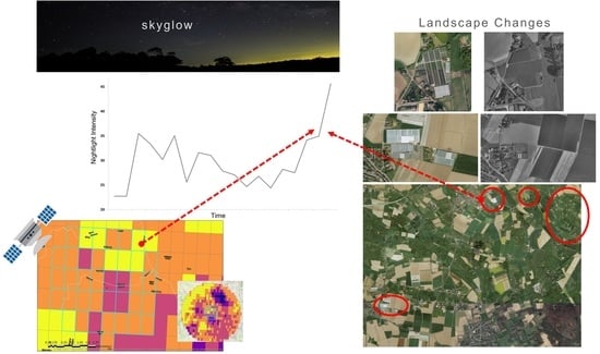
Figure 2.
Methodological workflow for processing DMSP-OLS data, analyzing pixel-level trends using linear regressions and the Mann–Kendall test, and refining the CORINE dataset to reflect urban and rural land cover. Combining the trend analyses with the urban/rural land cover classes served as the basis for investigating temporal and spatial trends at various scales. Further integrating aerial imagery, expert knowledge, and historical records provided a framework for attributing local changes in nightlight intensity to specific landscape features.

Figure 3.
Example of intercalibrated DMSP-OLS intensity data over the study area in the first (a, 1992) and second to last (b, 2009) years of the time series. The southeast portion of the study area (highlighted most in b) corresponds to the highest density urban areas.
Figure 3.
Example of intercalibrated DMSP-OLS intensity data over the study area in the first (a, 1992) and second to last (b, 2009) years of the time series. The southeast portion of the study area (highlighted most in b) corresponds to the highest density urban areas.

Figure 4.
Classification of rural (blue) and urban (transparent) areas based on the 2012 CORINE land cover data within a 10 km buffer around the insect trap locations. Urban classification is based on the reassignment of urban classes from the original CORINE dataset and their spatial relationships to city administrative units. The majority of the study area was classified as rural.

Figure 5.
Mann–Kendall tau statistic across the region for the full time period; values closer to −1 and 1 represent more significant trends and values closer to 0 are less significant. Positive and negative values represent the directionality of monotonic trends.
Figure 5.
Mann–Kendall tau statistic across the region for the full time period; values closer to −1 and 1 represent more significant trends and values closer to 0 are less significant. Positive and negative values represent the directionality of monotonic trends.

Figure 6.
Median nightlight intensity from the early time period (a, 1992–1999) and late time period (b, 2003–2010).
Figure 6.
Median nightlight intensity from the early time period (a, 1992–1999) and late time period (b, 2003–2010).

Figure 7.
The spatial distribution of the relative difference in nightlight intensity for each pixel between the early time period (1992–1999) and late time period (2003–2010) derived through linear trend analysis (a). The distribution (frequency) of the relative difference in nightlight intensity for all pixels is shown below (b), where the mean relative difference (red line) was approximately a 7% increase in nightlight intensity.

Figure 8.
Proportion of pixel increases in nightlight intensity exceeding various percent change thresholds observed between the early (1992–1999) and late (2003–2010) time periods.
Figure 8.
Proportion of pixel increases in nightlight intensity exceeding various percent change thresholds observed between the early (1992–1999) and late (2003–2010) time periods.

Figure 9.
Increases of nightlight intensity across urban (top) and rural (bottom) areas between 1992 and 2010 using Mann–Kendall tau statistic.
Figure 9.
Increases of nightlight intensity across urban (top) and rural (bottom) areas between 1992 and 2010 using Mann–Kendall tau statistic.

Figure 10.
Trends in nightlight intensity examined for evaluation points (pixels) which reflect patterns in land use change, showing decreasing trends in the early time period (1992–1999), and increasing trends in the late time period (2003–2010). Values on the right correspond to individual raster cell IDs.

Publisher’s Note: MDPI stays neutral with regard to jurisdictional claims in published maps and institutional affiliations. |
© 2022 by the authors. Licensee MDPI, Basel, Switzerland. This article is an open access article distributed under the terms and conditions of the Creative Commons Attribution (CC BY) license (https://creativecommons.org/licenses/by/4.0/).
Share and Cite
MDPI and ACS Style
LaRoe, J.; Holmes, C.M.; Schad, T. Nightlight Intensity Change Surrounding Nature Reserves: A Case Study in Orbroicher Bruch Nature Reserve, Germany. Remote Sens. 2022, 14, 3876. https://doi.org/10.3390/rs14163876
AMA Style
LaRoe J, Holmes CM, Schad T. Nightlight Intensity Change Surrounding Nature Reserves: A Case Study in Orbroicher Bruch Nature Reserve, Germany. Remote Sensing. 2022; 14(16):3876. https://doi.org/10.3390/rs14163876
Chicago/Turabian StyleLaRoe, Jillian, Christopher M. Holmes, and Thorsten Schad. 2022. "Nightlight Intensity Change Surrounding Nature Reserves: A Case Study in Orbroicher Bruch Nature Reserve, Germany" Remote Sensing 14, no. 16: 3876. https://doi.org/10.3390/rs14163876
Note that from the first issue of 2016, this journal uses article numbers instead of page numbers. See further details here.