Real-Time Weed Control Application Using a Jetson Nano Edge Device and a Spray Mechanism

Abstract

Portable devices play an essential role where edge computing is necessary and mobility is required (e.g., robots in agriculture within remote-sensing applications). With the increasing applications of deep neural networks (DNNs) and accelerators for edge devices, several methods and applications have been proposed for simultaneous crop and weed detection. Although preliminary studies have investigated the performance of inference time for semantic segmentation of crops and weeds in edge devices, performance degradation has not been evaluated in detail when the required optimization is applied to the model for operation in such edge devices. This paper investigates the relationship between model tuning hyperparameters to improve inference time and its effect on segmentation performance. The study was conducted using semantic segmentation model DeeplabV3 with a MobileNet backbone. Different datasets (Cityscapes, PASCAL and ADE20K) were analyzed for a transfer learning strategy. The results show that, when using a model hyperparameter depth multiplier (DM) of 0.5 and the TensorRT framework, segmentation performance mean intersection over union (mIOU) decreased by 14.7% compared to that of a DM of 1.0 and no TensorRT. However, inference time accelerated dramatically by a factor of 14.8. At an image resolution of $1296\times 966$, segmentation performance of 64% mIOU and inference of 5.9 frames per second (FPS) was achieved in Jetson Nano’s device. With an input image resolution of $513\times 513$, and hyperparameters output stride OS = 32 and DM = 0.5, an inference time of 0.04 s was achieved resulting in 25 FPS. The results presented in this paper provide a deeper insight into how the performance of the semantic segmentation model of crops and weeds degrades when optimization is applied to adapt the model to run on edge devices. Lastly, an application is described for the semantic segmentation of weeds embedded in the edge device (Jetson Nano) and integrated with the robotic orchard. The results show good spraying accuracy and feasibility of the method.

1. Introduction

Weed control is a practice aimed at reducing competition among plants for water and nutrients. Cultivation techniques to control the development of weeds are commonly referred to as soil management. The application of herbicides at the beginning of the vegetative cycle is especially important in weed control because it is one of the critical factors for success [1]. Automatic weed detection is one of the viable solutions for the efficient reduction in or exclusion of chemical products in the field. Studies have focused on modern approaches that automatically analyze and evaluate weeds in images (e.g., crop and weed segmentation).

Edge computing approaches have been proposed where the computation of data is performed locally, as in robots for agriculture. Examples of technical and technological solutions that can benefit from this approach can be found in [2,3,4,5,6,7,8,9,10,11,12]. Furthermore, it is desired to balance accuracy, throughput, and power management, which is essential in various fields such as the Internet of Things (IoT), robotics, autonomous driving, and drone-based surveillance [13]. Most modern computer vision systems for weed control are based on desktop computers (i.e., the computer is heavy, not portable, and must be connected to the power grid) [14,15,16,17,18]. This means that these systems are heavy, expensive, and require much electrical power. These problems render this approach (i.e., desktop-based) impractical for use in small and low-cost orchard robots.

Milioto et al. [14] proposed an encoder–decoder model based on convolutional neural networks (CNNs) for crop and weed segmentation. They used RGB images and produced the excess green, excess red, color index of vegetation extraction, and normalized difference vegetation indices as inputs to the model. The best performance was 59% mean intersection over union (mIOU) on the desktop device, and an inference time of 190 ms on the Jetson TX2. This model is relatively heavy compared to others, being able to perform only 5.2 frames per second (FPS) inferences at an image resolution of $512\times 384$ on the Jetson TX2 device.

McCool et al. [15] implemented a lightweight segmentation model based on deep convolutional neural networks (DCNNs) that could be used in robotic platforms to segment crops and weeds in images. They used a desktop computer with a graphics processing unit (GPU) card for training and inference. The model was trained on the Crop Weed Field Image Dataset (CWFID) with an image resolution of $1296\times 966$, and achieved an accuracy of 93.9% with an inference time of 8.33s using an Inception-v3 backbone.

Khan et al. [16] proposed the CED-NET encoder–decoder semantic segmentation method for crop and weed segmentation. Their model had four networks, where two networks are trained independently for segmenting crops, and the other two for weeds. They claimed that this approach to extract features at different scales provides coarse-to-fine predictions and reduces the number of network parameters. Using a desktop with a GPU, they achieved a performance of 77% mIOU in the CWFID dataset.

Wang et al. [17] implemented an encoder–decoder deep-learning network for pixelwise semantic segmentation of crops and weeds. In addition, three images pre-processing were proposed to improve the model performance. They investigated the model by training and testing in two different datasets: sugar beet and oilseed. The best segmentation performance was 89% mIOU. Using a desktop with a GPU, the inference time for an image with a dimension of $1296\times 966$ was 100 ms.

Fawakherji et al. [18] proposed a deep-learning-based method for crop and weed classification using two different convolutional neural networks (CNNs). The first network performs pixelwise segmentation between vegetation and soil. After segmentation, each plant is classified into crops or weeds using the second network. For the semantic segmentation network, they used the UNet structure with the VGG16 backbone. For the classification network, they used a fine-tuned model of VGG16 that leveraged deep CNN’s object classification capabilities. For training and testing, they used the NVIDIA GTX 1070 GPU and achieved 87% correctly detected crops and 77% correctly detected weeds.

Olsen [19] proposed a real-time weed control system for a mobile robot. The author used a set of deep neural networks to classify nine types of weed images. In the Jetson Nano device, the MobileNetV2 model achieved an inference time of 29.0 ms; the ResNet-50 architecture achieved an inference time of 59.8 ms; the Inception model ran at 91.9 ms; and the VGG16 model achieved an inference speed of 166.3 ms. This work addresses the problem of image classification. That is, the model performs inference on whether weeds are present and which type they are. However, there is no spatial information (location) about the detected weeds in the image, unlike the semantic segmentation model.

Partel et al. [20] developed an innovative sprayer that uses object detector Tiny Yolov3 to distinguish target portulaca plants, sedge weeds, from nontarget pepper plants and precisely spray to the desired location. Using an NVIDIA Jetson TX2 device and an image resolution of $1024\times 256$, it achieved overall precision and recall of 59% and 44%, respectively, and the framework could handle 22 FPS. The experiment was carried out in a simulated field of crops and weeds that did not correspond to the natural environment, which is normally a dense vegetable field.

Using the SegNet encoder–decoder network for semantic segmentation, Abdalla et al. [21] conducted a study on weed segmentation using fine-tuning and data-augmentation techniques. They used SegNet with a VGG16 backbone at an image resolution of $3888\times 5184$, and the model achieved an inference time of 230 ms (i.e., 4.3 FPS) and mIOU of 87% in a desktop computer equipped with a GPU card.

Asad and Bais [22] used the SegNet and UNET semantic segmentation models with VGG16 and ResNet-50, classifying crop and background pixels as one class, and all other vegetation as the second class. At an image resolution of $1440\times 960$, the SegNet model based on ResNet-50 showed the best results with an mIOU of 82%. The experiments were performed on a desktop computer equipped with a GPU card, and the authors did not report the inference time.

Ma et al. [23] used the SegNet semantic segmentation model based on a fully convolutional network with the AlexNet backbone to segment rice seedlings, weeds, and the background. At an image resolution of $912\times 1024$, the model achieved an mIOU of 62% and an inference time of 0.6 s (it could process 1.6 FPS). The experiments were performed on a desktop computer equipped with a GPU card.

Lameski et al. [24] presented a carrot–weed dataset with RGB images of young carrot seedlings. The dataset contains 39 images with the same size of $3264\times 2448$. The dataset consists of 311,620,608 pixels, comprising 26,616,081 pixels of carrot plants, 18,503,308 pixels of weed plants, and 266,501,219 pixels of soil. The authors conducted the initial experiments on the dataset using the SegNet semantic segmentation model and achieved the best accuracy of 0.641 for the segmentation of weeds, plants, and soil. In this work, there is no information about the inference time and the device for training and inference.

Naushad et al. [25] used VGG16 and wide residual networks (WRNs) to classify land use and land cover in RGB band images (at $64\times 64$ resolution) from the EuroSAT dataset. A transfer-learning technique was used to improve the accuracy. The best accuracy was achieved by the WRN model with 99.17%.

Nanni et al. [26] proposed an ensemble method for semantic segmentation combining DeepLabV3, HarDNet-MSEG, and Pyramid Vision Transformers. The model was trained and evaluated on different datasets covering five scenarios: polyp detection, skin detection, leukocyte recognition, environmental microorganism detection, and butterfly recognition. According to the authors, the model provides state-of-the-art results.

Autonomous mobile robots use remote-sensing techniques and technologies for several agricultural tasks such as monitoring, fertilizing, herbicide spraying, or harvesting.

Computer vision applications can run on mobile devices by using deep-learning frameworks (e.g., TensorRT or Tensorflow Lite) and accelerators. For this, some optimization is needed in the original or standard computer-vision models to minimize memory and computational footprints [27]. 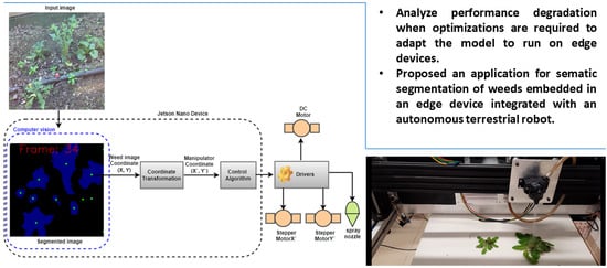Although preliminary studies investigated the inference performance for the semantic segmentation of crops and weeds in mobile edge devices [14,19,20], to the best of our knowledge, no study has been conducted to show the performance degradation (mIOU) when applying the required optimization to the model to operate in such edge devices. The purpose of this study is to:

• Perceive the relationship between the model tuning hyperparameters of the DeeplabV3 semantic segmentation model with MobileNet backbone to improve inference time and its impact on segmentation performance (using the mIOU metric).
• Evaluate the suitability of the Cityscapes, PASCAL, and ADE20K datasets for a transfer-learning strategy in crop and weed segmentation.
• Propose and evaluate a real-time weed control application using a Jetson Nano Edge device and a spray mechanism.

The remainder of this paper is organized as follows. The hardware used to train and infer the model, the dataset used, an explanation of the semantic segmentation model, including the used backbone, the model optimization, and the practical application, are presented in Section 2. The results of the proposed model when applied to the weed datasets and the practical application are presented along with the related analysis and discussion in Section 3. The conclusion of the paper is in Section 4.

2. Materials and Methods

2.1. Resources for Network Training and Deployment

A desktop computer with an Intel Core i7-4790 CPU (3.60 GHz), GeForce RTX 2080 8 GB GPU, 16 GiB RAM, and Ubuntu 18.04 was used for training and obtaining the base model.

A Jetson Nano edge device was used for the deployment. NVIDIA’s Jetson family features a heterogeneous CPU–GPU architecture, small form factor, light weight, and low power consumption, and is one of the most widely used edge device families with accelerators for machine-learning inference. It can run neural networks in parallel for applications such as image classification, object detection, and segmentation (Mittal, 2019). It works with an inserted micro-SD card with the system image.

Table 1. Technical specifications of Jetson Nano.

Item	Spec
AI performance	472 GFLOPs
GPU	128-core NVIDIA
CPU	Quad-Core Arm
Memory	4 GB 64-bit
Power	5 W|10 W

shows the technical specifications of the Jetson Nano Developer Kit.

Figure 1 shows the general outline of this work, starting with the acquisition and preparation of the dataset (Figure 1A). The model was trained to obtain the base models (Figure 1B). Then, the model was optimized (post-training) (Figure 1C). Lastly, the model was deployed on the Jetson Nano device (Figure 1D). The next subsections provide more details.

2.2. Dataset

Two datasets were used in this work: CWFID (Section 2.2.1) and the Weeds dataset (Section 2.2.2). The CWFID was used to investigate how a model degrades when optimization is applied to adapt the model to run in edge devices, and the Weeds dataset was used for the real-time application proposal.

2.2.1. CWFID

The benchmark Crop Weed Field Image Dataset (CWFID) [28] consists of crops (carrots) and weeds. It was used to train and evaluate the models. For each image, a manual annotation (ground truth) per pixel (e.g., green mask for crops, and red mask for weeds) is available for crops and weeds.

Table 2. Scope of the CWFID dataset and split.

Parameter	Value
Number of images	60
Number of labeled plants	494
Number of labeled crop	162
Number of labeled weed	332
Dataset split
Number of training images	42
Number of test images	18

and

Table 3. CWFID dataset pixels information.

Item	Back Ground	Weed Class	Crop Class
Total of pixels	69,580,840	4,322,897	1,212,423
Training pixels	49,922,402	3,093,709	817,137
Test pixels	19,658,438	1,229,188	395,286

summarize the details of the dataset.

2.2.2. Weed Dataset for Real-Time Application

A weed dataset was assembled to train the model for the real-time application experiment. The images were captured using a Sony DSC-RX100M2 camera. A total of 12 RGB images were selected and resized into a resolution of $513\times 513$ (the input size of the pretrained model used for fine tuning). Subsequently, the images were manually labeled. Figure 2 shows two examples of images in the weed dataset for the real-time application experiment. The images are shown at the top, and the respective image, labeled weed (i.e., ground-truth mask), is shown at the bottom.

Table 4. Scope of the weed dataset for the real-time experiment.

Parameter	Value
Number of images	12
Number of labeled weeds	847
Dataset split
Number of training images	10
Number of validation images	2

and

Table 5. Information about the pixels of the weed dataset.

Item	Background	Weed Class
Total of labeled pixels	25,934,802	1,789,998

summarize the weed dataset for the real-time application experiment.

2.3. DeepLab Model and Training

2.3.1. Semantic Segmentation

Semantic segmentation is a dense prediction task that assigns semantic labels to each pixel in an image [29]. Some state-of-the-art models are based on an encoder–decoder network structure, as shown in Figure 3. Encoder–decoder is a group of models that learn to map data from an input space to an output space over a two-level network [30].

Long et al. [29] developed a method for semantic segmentation by adapting a deep-learning classification network to perform dense prediction. A fully convolutional network (FCN) generates coarse output maps with reduced dimensions (i.e., downsampling). The feature maps are brought back to the input size by stacking deconvolutional layers (i.e., upsampling).

An encoder–decoder semantic segmentation model for medical images, U-NET, was developed by Ronneberger et al. [31]. Similarly, in [29], an FCN was used in the encoder part to capture contextual information. In this phase, due to the max-polling operation, the feature maps are contracted. In the decoder, successive expansion is performed using the mirrored structure of the encoder, but upsampling operators replace max polling.

Chen et al. [32] proposed a semantic segmentation model that combines the responses at the last CNN layer with a fully connected conditional random field (CRF). This approach adds more context to the model and helps in locating segment boundaries with better accuracy. In [30] contains the main semantic segmentation strategies.

Defining a network backbone while considering the most important aspects for a particular application is a crucial task. In our study, time is an important aspect, since the application needs to perform inferences in real-time. Another aspect is the lightness of the model, since the hardware is a small, low-cost, and low-power portable device with limited processing power (cores) and memory. Considering these aspects, the MobilenetV2 [33] was selected, as it met these specifications.

In this work, state-of-the-art semantic segmentation model DeepLabV3 [34] was employed with the MobilenetV2 backbone by using the Tensorflow Model Garden (TMG) framework [35] to perform the experiments. The DeelLabV3 was chosen because it is a very versatile model where the Mobilenet backbone could be used for the purposes of this work, such as model shrinking with hyperparameters. Figure 4 illustrates the architecture of the DeepLabV3 model, as originally described.

2.3.2. Network Backbone

In an image segmentation model based on deep learning, the first part consists of a DCNN. Its main goal is to extract features from the input image. This feature extractor is usually referred to as the backbone of the model. In this work, the MobilenetV2 DCNN was used as the backbone. The architecture of MobilinetV2 was customized by adjusting the depth multiplier (DM) and output stride (OS) hyperparameters to achieve the desired performance for the application (i.e., light weight and fast inference time). To optimize the model for light weight, the DM hyperparameter for model shrinkage was adjusted. In particular, the DM hyperparameter affects the number of model input channels for each layer. For example, at DM = 1.0, the model had the original number of input channels; at DM = 0.5, the model had half the number of input channels. In this study, the experiments were conducted with DM = 1.0 and DM = 0.5. In addition, the DeepLabV3 model implements atrous convolution to explicitly control how densely features should be computed rather than using pooling in a fully convolutional network. The OS hyperparameter is the ratio of the size of the input image and the size of the last output feature map in the encoder. Values of 8, 16, and 32 were used for OS to investigate the trade-off between accuracy and inference time, as this hyperparameter affects segmentation accuracy and inference time.

2.3.3. Network Training

Software tools were Python 3.6 with the TensorFlow Deep Learning package and the Tensorflow Model Garden (TMG) framework. Using a fine-tuning strategy is more effective than training deep networks from scratch [36]. In this work, we performed fine tuning as recommended in [36]. TMG provided a fine-tuning strategy to train the last layers of the DeepLabV3 model for a new segmentation dataset. DeepLabV3 was trained on the basis of pretrained models on the Cityscape [37], ADE20k [38], and PASCAL [39] datasets to reduce training time and investigate which of these models provided the best segmentation results. The training configurations were as suggested in [35]. Specifically, ADAM learning rate = 0.001, ADAM momentum = 0.9, ADAM epsilon = $1\times {10}^{-8}$, and base learning rate of 0.0001 were used for 30,000 iterations with a batch size of 2.

2.4. Post-Training Optimization

After training, the TMG framework provided a set of checkpoint files (i.e., the trained model). Then, the checkpoint files were converted into a frozen graph using a tool (script) available in the TMG framework. Then, the frozen graph was converted (optimized) to run on the Tensorflow Real-Time (TensorRT) engine using the TensorRT class converter.

TensorRT is a software development kit (SDK) developed by NVIDIA Corporation to optimize inference time for deep learning on NVIDIA graphics processing units (GPUs) [40]. It works on top of already trained networks by combining layers and optimizing kernel selection to improve latency, output capacity, energy efficiency, and memory consumption [41]. An example of TensorRT optimization is model quantization from 32-bit floating-point numbers to 16-bit (FP16) or 8-bit integers (INT8). In addition, TensorRT performs on an optimized inference engine based on a trained network.

2.5. Model Assessment

2.5.1. Computation Footprint

The metric of floating-point operations (FLOPs) was used to measure the computational complexity of the models, where addition and multiplication were both considered as one FLOP [42]. The number of FLOPs required by the model to perform an inference is an indicator of model latency, which is reflected in the inference time.

2.5.2. Segmentation Performance

The metric used to evaluate pixelwise segmentation performance is (mIOU), defined by Equation (1):

$$\mathrm{mIOU}=\frac{1}{C}\sum _{i=1}^C\frac{T{P}_i}{T{P}_i+F{P}_i+F{N}_i},$$

(1)

where $TP$ stands for true positive, $FP$ stands for false positive, $FN$ stands for false negative, and C is the number of classes.

2.6. Real-Time Application

The semantic segmentation model (computer vision) was integrated into the robotic orchard rover developed by Veiros et al. [43] (Figure 5). The goal of this experiment was to investigate the accuracy and feasibility of the computer-vision framework in conjunction with a mechanism for applying a herbicide spray to weeds. The experiments were conducted in the laboratory.

2.6.1. Mechanism

Figure 6 shows the main components of the Cartesian robotic manipulator for spray applications. Three actuators must be controlled by the output pins of the Jetson Nano device: pressure motor: a DC motor that applies pressure to the herbicide container; manipulator motor: a stepper motor that moves the axis of the Cartesian manipulator; nozzle relay: a relay that opens and closes the spray valve; spray nozzle; Cartesian robot manipulator; herbicide container.

2.6.2. Camera

A Raspberry Pi v2 camera module with a Sony IMX219 8-megapixel sensor was used to capture the video images. Figure 7 shows the camera location embedded on the robotic orchard rover.

2.6.3. Computer Vision and Mechanism Integration

The DeepLabV3 model was trained with the dataset described in Section 2.2.2 for practical application. Training was performed as described in Section 2.3.3, fine tuning on the PASCAL dataset, with hyperparameters OS = 16 and DM = 1.0. Although the dataset consisted of only a few images, each image contained many labeled weeds (see Figure 2). Another fact that allows for training deep learning models with few data is the use of a fine-tuning strategy.

Figure 8 provides a general view of the practical experiment involving integration between the computer vision and the mechanism. The output of the computer-vision model was a segmented image with a set of (X, Y) coordinates (centroid) of each weed (green dots). These coordinates were converted into the manipulator’s Cartesian manipulator coordinates (X’, Y’). The (X’, Y’) coordinates were then fed into the control algorithm that calculated the sequence of movements to position the spray nozzle on the detected weed and execute the spray.

2.6.4. Coordinate Transformation

The spray nozzle was attached to the Cartesian axis of the robot manipulator. The axis was driven by the stepper motorX’ (Figure 8), which was configured to perform one revolution when 1000 pulses are applied. The image output from the computer-vision framework had a resolution of $513\times 513$.

For the spray nozzle to cover the spatial camera view, the stepper motor X’ should receive 4350 steps. This relationship is shown in Figure 9. Given an (X, Y) weed position in the image, the number of pulses (steps) that must be applied to stepper motor X’ for the nozzle to hit the weed position is calculated by Equation (2).

$$Pulses=\frac{4351}{513}\times \mathrm{X},$$

(2)

where X stands for the position of the weed in the image. That means that the coordinate transformation converts the pixel position into the number of pulses (steps).

3. Results and Discussions

This section presents the results of the DeepLabv3 experiments on the semantic segmentation of the WCFID dataset where hyperparameters were set, an optimization framework was applied, and fine tuning was performed.

3.1. Pretrained Models and Fine-Tuning Performance

To investigate how the pretrained models affected segmentation performance for the use case (i.e., crop and weed segmentation), experiments were conducted with the fine-tuning strategy using the Cityscape, ADE20k, and PASCAL datasets.

Table 6. Fine-tuning comparison (mIOU).

Pre-Trained Dataset	OS = 8	OS = 16	OS = 32
PASCAL	75%	72%	66%
ADE20k	76%	74%	68%
Cityscape	78%	74%	68%

shows the results for this experiment in combination with hyperparameters OS and DM = 1.0.

As shown in Table 6, when fine tuned using hyperparameter OS = 8, the Cityscape dataset performed the best with 78% mIOU. However, when using OS = 16 and OS = 32, the performance for fine tuning with Cityscape and ADE20k was the same. OS = 8 gave the best result compared to OS = 16 and OS = 32 because it captured more spatial information from the input. The fine-tuning process uses knowledge gained from pretraining in other datasets. For example, the Cityscape dataset likely had more similarities with plants, e.g., the Vegetation class in the Nature group, which is probably the reason for the best result.

3.2. Model Optimization and Performance Degradation

This experiment investigates the relationship between model optimization (i.e., tuning hyperparameters and applying the TensorRT framework to improve inference time) and segmentation degradation. Although fine tuning with the Cityscape dataset gave the best results, as shown in a previous experiment, fine tuning in this experiment was used for the PASCAL dataset because a pretrained model with DM = 0.5 and DM = 1.0 was only available for the PASCAL dataset [44].

Table 7. Temporal computational cost (in GFLOPs) with different parameterisations.

Optimization	OS = 8	OS = 16	OS = 32
DM = 1.0	81.9	25.1	14.7
DM = 0.5	26.1	7.9	4.4

shows the computational cost of each model measured in giga floating-point operations (GFLOPs). It is clear how much the optimization reduced the computational cost: using hyperparameters DM = 0.5 and OS = 32 in the CNN backbone, the computational cost of the model was reduced from 81.9 to 4.4 GFLOPs. This performance was due to the reduction in convolutional layers in the MobileNet backbone by hyperparameters DM, which shrank the model by a factor of 0.5, and OS.

Table 8. Summary of segmentation performance with respect to different tested parameterisations.

Optimization	OS = 8	OS = 16	OS = 32
DM = 1.0	75%	72%	66%
DM = 1.0 + TensorRT	-	72%	66%
DM = 0.5	73%	68%	64%
DM = 0.5 + TensorRT	-	68%	64%

shows how segmentation performance is affected by optimization to reduce inference time. The best model segmentation performance was 75% mIOU for the model with OS = 8 and DM = 1.0. The worst performance was 64% mIOU for the model with successive and more stringent optimization to improve the inference time, i.e., depth multiplier of 0.5, output stride of 32, and TensorRT. Reducing the model size to achieve fast inference time by using DM = 0.5 and OS = 32 led to a decrease in segmentation accuracy. The model became shallower and lost information about the features of the input image. An important result is also that using the TensorRT framework for enhancement did not affect the segmentation accuracy. TensorRT is an inference-oriented framework whose main purpose is efficient inference. It also supports dynamic graphs, which enables the efficient reuse of memory and improves inference performance [27].

The corresponding segmentation quality results are shown in Figure 10. Segmentation performance (quality) varied with different hyperparameters DM and OS. Comparing the results with the same OS but different DM (i.e., (c) with (h), (d) with (i), and (e) with (j)), the results with DM = 0.5 had more mis-segmentations between crops and weeds than those with DM = 1.0. This result can be explained by the fact that the DM hyperparameter affected the complexity of the model (size). A model with DM = 1.0 was deeper than a model with DM = 0.5.

If we now compare the results with the same DM but different OS (8, 16 and 32), we can see that the results with O = 8 were finer (fine details) than those with OS = 16 and OS = 32. The results with OS = 16 were finer than those of models with OS = 32. This result can be explained by the fact that the OS hyperparameter influenced the sparsity of the input calculation of the model.

Table 9. Inference time performance (s).

Optimization	OS = 8	OS = 16	OS = 32
DM = 1.0	2.51	0.85	0.77
DM = 1.0 + TensorRT	-	0.57	0.31
DM = 0.5	1.19	0.43	0.33
DM = 0.5 + TensorRT	-	0.3	0.17

shows how optimization affected the time of model inference. The best result was 0.17 s using DM = 0.5, OS = 32 and TensorRT. Table 7 shows that this configuration resulted in the smallest model, which reduced the inference time, as expected.

Table 10. Variation in inference time with respect to different parameterisations when compared to the baseline configuration.

Optimization	OS = 8	OS = 16	OS = 32
DM = 1.0	1	3.0	3.3
DM = 1.0 + TensorRT	-	4.4	8.1
DM = 0.5	2.1	5.8	7.6
DM = 0.5 + TensorRT	-	8.4	14.8

and

Table 11. Variations in model performance (mIOU%) with respect to different parameterisations considering the optimal configuration tested.

Optimization	OS = 8	OS = 16	OS = 32
DM = 1.0	0	−4.0	−12.0
DM = 1.0 + TensorRT	-	−4.0	−12.0
DM = 0.5	−3.0	−9.3	−14.7
DM = 0.5 + TensorRT	-	−9.3	−14.7

show the relationship (correlation) between model segmentation performance and inference time. The inference time could be accelerated by a factor of 14.8, while the segmentation performance (mIOU) decreased by 14.7%. With these optimizations and an image resolution of $1296\times 966$, the model could perform segmentation in 5.9 FPS.

In addition, the results were compared with previously published segmentation work in the CWFID dataset. In

Table 12. Comparison of the segmentation performance of other works on the CWFID test dataset. DeepLabV3* (OS = 8 and DM = 1.0) and DeepLabV3** (OS = 32 and DM = 0.5).

Model	Input Size	GPU	Accuracy	mIOU	FPS
Adapted-IV3 [15]	1296 × 966	Titan X	93.9%	-	0.12
CED-Net [16]	1296 × 966	Titan XP	-	77%	-
DeepLabV3*	1296 × 966	Maxwell	-	75%	0.4
DeepLabV3**	1296 × 966	Maxwell	-	64%	5.9

, Maxwell is a very small 128-core GPU integrated into the Jetson Nano developer kit, while Titan X is a standard 3584-cores GPU and Titan XP a 3840-cores GPU board.

For work comparison, Table 12 shows the input size of the image, the GPU capabilities, the segmentation performance of the model in terms of accuracy or mIOU, and the inference performance FPS. Regarding GPU characteristics, our approach (DeepLabV3) uses the Maxwell embedded in the Jetson Nano, which is a portable device. In contrast, the other approaches use GPU cards that function in conjunction with a desktop.

Regarding the segmentation performance of the models, CED-Net and our model could be compared because the value of the results is presented in the same metric (mIOU). CED-Net outperformed our approach (DeepLabV3*) by only 2%.

Inference time performance could be compared between our approach and Adapted-IV3. Our approach (DeepLabV3**) outperformed Adapted-IV3 by about 50 times. The primary key to this performance is the use of the MobileNet backbone in the encoder part of the DeepLabV3 model, since the MobileNet DCNN provides light weight by performing depthwise separable convolutions. Another contribution to this performance was the setting of hyperparameters DM = 0.5 and OS = 32, and the use of the TensorRT framework.

3.3. Image Scale Analysis

In addition, smaller input images were considered to evaluate the inference time under this condition. The experiment was performed by cropping the WCFDI images in their center to a resolution of $513\times 513$.

Table 13. Analysis of inference time with respect to the size of the input (s).

Optimization	OS = 8	OS = 16	OS = 32
DM = 1.0	0.54	0.18	0.12
DM = 1.0 + TensorRT	0.27	0.09	0.07
DM = 0.5	0.54	0.12	0.06
DM = 0.5 + TensorRT	0.27	0.07	0.04

shows these results. For the quality segmentation shown in Figure 11, an inference time of 0.04 s was achieved, corresponding to processing of 25 FPS.

3.4. Real-Time Application

The goal of this experiment was to demonstrate a practical application of the deep-learning-based computer-vision model, its reliability in real-time, and its integration with mechanical control.

After weeds had been detected by the computer-vision model, a series of actuators were controlled in sequence (e.g., the manipulator motor and the spray solenoid valve). The response time of each actuator was considered by setting the required delay time to finish the current step and start the next step.

We simulated a field soil with weeds by manually positioning them in the camera’s field of view. Figure 12 shows the general view of the experiment. The window in which the input image coming from the camera is displayed. The window in which the segmented image is displayed. The area where the weed was placed.

Figure 13 illustrates the test result for a single image of the image acquisition. In (A), an image with two weeds is shown. In (B), two weeds were segmented with a high-quality border corresponding to the image in (A). The green dots in the center of the blue segmented regions are the references (location coordinates) for the Cartesian manipulator, as described in Section 2.6.4. (C) shows the weeds in the field of view of the camera and the spray nozzle.

Figure 14 shows a sequence of four images. The upper-left partial image (Frame: 189) is an image without weeds. The remaining images (frame: 224, frame: 226, and frame: 241) show the image with the weeds (input) and the corresponding segmentation results (output). The blue segmented areas had high shape similarity with the corresponding weed image. The green dots indicating the center of gravity of the weeds are clearly visible in the center of each segmented area. Thus, these results show the good accuracy of the computer-vision model.

The computer-vision model was used in the Jetson Nano device to determine the reference position of the weeds for mechanism control (see Section 2.6.3 and Section 2.6.4). Given a set of weed references, the Cartesian manipulator positioned the nozzle on the particular weed and performed the spraying. Figure 15 shows the exact positioning of the nozzle and the spray.

A video demonstration of the experiment result is available in the data-availability statement at the end of the manuscript.

3.5. Final Discussions

Taken together, these results provide important insights into the semantic segmentation accuracy and inference time performance of crop and weed detection when the necessary optimizations are conducted to the model to run it on edge devices. At the cost of worse segmentation performance, inference time can be dramatically increased, enabling real-time inference. The approach proposed in our study can render the inference time faster than that of the compared models even though it is a portable device, while the others are desktop-based. Compared to an approach with similar hardware and input size [14], our proposed approach performed inference about 5 times faster. DeepLabV3 proved to be a very versatile model for segmentation tasks, since the trade-off between segmentation accuracy and inference time can be controlled by hyperparameters OS and DM.

In addition, fine tuning the model in the Cityscapes, PASCAL, and ADE20K datasets yielded good results. Cityscapes provided the marginally best performance compared to the PASCAL and ADE20K datasets. The results show that, when accuracy requirements are high, fine tuning with the pretrained Cityscape dataset is the best solution. If time inference is a requirement, then the best approach is to fine-tune with the pretrained Cityscape or ADE20k dataset, since both achieved the same accuracy performance. In the latter case, it is recommended to fine-tune with the PASCAL dataset if Cityscape and ADE20k are not available. Real-time application for weed spraying was also accurate and feasible. The segmentation model embedded in the edge device provided all the information (position references) needed to control the mechanism. According to the video demonstration, the mechanism precisely positioned the nozzle at all target weeds and applied the spray.

4. Conclusions

Edge devices play an important role when mobility is required. Computer-vision models running on such devices must be optimized due to the device’s limitations in terms of memory and computation. There are many studies and proposals for the optimization of deep learning models, but there is still a lack of research on how the performance of the models is affected by optimization. Moreover, there are not yet many real-world use cases of computer vision and its interaction with mechanisms in the domain of agriculture.

In this work, the optimization of the semantic segmentation model for weed was investigated, and its effects on inference time and segmentation performance were studied. The procedure can be described by using crop and weed images for training and validating the model; the procedure was applied for training the DeeplabV3 semantic segmentation model with the fine-tuning approach. Model optimization was performed before and after training by selecting different model hyperparameters and applying model quantization. Lastly, the performance of the model was evaluated.

Experimental results show that, by using hyperparameters DM = 0.5 and OS = 32 in the CNN backbone, the computational cost of the model was reduced from 81.9 to 4.4 GFLOPs. On the Jetson Nano device, the best inference time of the model was 0.17 s. Compared to the baseline model (i.e., the model without optimization), the inference time was accelerated by a factor of 14.8, while the segmentation performance (mIOU) was decreased by 14.7%. This result illustrates the potential of the optimizations for building lightweight models that still have good predictive accuracy.

Since the technique of fine tuning is important when only a small amount of training data is available, the effects of fine tuning on pretrained models were investigated. With respect to the PASCAL and ADE20K datasets, Cityscapes achieved the marginally best performance.

An extension of this work is to propose a practical application using the weed segmentation model presented in this study, an edge device, and a spraying mechanism. The results show that the proposed method is feasible, and has good accuracy and potential for weed control.

The limitation of this study was that the Cartesian robot manipulator operates in only one axis, while in practice, the other axis motion is the translational motion performed by the robot wheels. Since the practical application was carried out in a simulated environment (laboratory), the main objective of future work is to develop a complete system to study the performance of weed control in a real agricultural environment.

The results presented in this study demonstrate the potential of using lightweight models and portable edge devices for the real-time semantic segmentation of weeds.

References

1. Simões, M. +Pêssego – Resultados de Apoio à Gestão; Technical Report; Centro Operativo e Tecnológico Hortofrutícola Nacional: Alcobaça, Portugal, 2017. [Google Scholar]
2. Alibabaei, K.; Gaspar, P.D.; Lima, T.M. Modeling evapotranspiration using Encoder-Decoder Model. In Proceedings of the 2020 International Conference on Decision Aid Sciences and Application (DASA), Sakheer, Bahrain, 8–9 November 2020; pp. 132–136. [Google Scholar]
3. Assunção, E.; Diniz, C.; Gaspar, P.D.; Proença, H. Decision-making support system for fruit diseases classification using Deep Learning. In Proceedings of the 2020 International Conference on Decision Aid Sciences and Application (DASA), Sakheer, Bahrain, 8–9 November 2020; pp. 652–656. [Google Scholar]
4. Shanmugam, S.; Assunção, E.; Mesquita, R.; Veiros, A.; Gaspar, P.D. Automated weed detection systems: A review. KnE Eng. 2020, 271–284. Available online: http://3.65.204.3/index.php/KnE-Engineering/article/view/7046 (accessed on 30 July 2022).
5. Cunha, J.; Gaspar, P.D.; Assunção, E.; Mesquita, R. Prediction of the Vigor and Health of Peach Tree Orchard. In Proceedings of the International Conference on Computational Science and Its Applications, Cagliari, Italy, 13–16 September 2021; Springer: Cham, Switzerland, 2021; pp. 541–551. [Google Scholar]
6. Mesquita, R.; Gaspar, P.D. A Novel Path Planning Optimization Algorithm Based on Particle Swarm Optimization for UAVs for Bird Monitoring and Repelling. Processes 2021, 10, 62. [Google Scholar] [CrossRef]
7. Alibabaei, K.; Gaspar, P.D.; Lima, T.M. Modeling soil water content and reference evapotranspiration from climate data using deep learning method. Appl. Sci. 2021, 11, 5029. [Google Scholar] [CrossRef]
8. Alibabaei, K.; Gaspar, P.D.; Lima, T.M. Crop yield estimation using deep learning based on climate big data and irrigation scheduling. Energies 2021, 14, 3004. [Google Scholar] [CrossRef]
9. Alibabaei, K.; Gaspar, P.D.; Lima, T.M.; Campos, R.M.; Girão, I.; Monteiro, J.; Lopes, C.M. A Review of the Challenges of Using Deep Learning Algorithms to Support Decision-Making in Agricultural Activities. Remote Sens. 2022, 14, 638. [Google Scholar] [CrossRef]
10. Alibabaei, K.; Gaspar, P.D.; Assunção, E.; Alirezazadeh, S.; Lima, T.M. Irrigation optimization with a deep reinforcement learning model: Case study on a site in Portugal. Agric. Water Manag. 2022, 263, 107480. [Google Scholar] [CrossRef]
11. Alibabaei, K.; Gaspar, P.D.; Assunção, E.; Alirezazadeh, S.; Lima, T.M.; Soares, V.N.; Caldeira, J.M. Comparison of On-Policy Deep Reinforcement Learning A2C with Off-Policy DQN in Irrigation Optimization: A Case Study at a Site in Portugal. Computers 2022, 11, 104. [Google Scholar] [CrossRef]
12. Alibabaei, K.; Assunção, E.; Gaspar, P.D.; Soares, V.N.; Caldeira, J.M. Real-Time Detection of Vine Trunk for Robot Localization Using Deep Learning Models Developed for Edge TPU Devices. Future Internet 2022, 14, 199. [Google Scholar] [CrossRef]
13. Mittal, S. A Survey on optimized implementation of deep learning models on the NVIDIA Jetson platform. J. Syst. Archit. 2019, 97, 428–442. [Google Scholar] [CrossRef]
14. Milioto, A.; Lottes, P.; Stachniss, C. Real-Time Semantic Segmentation of Crop and Weed for Precision Agriculture Robots Leveraging Background Knowledge in CNNs. In Proceedings of the 2018 IEEE International Conference on Robotics and Automation (ICRA), Brisbane, Australia, 21–25 May 2018; pp. 2229–2235. [Google Scholar] [CrossRef]
15. McCool, C.; Perez, T.; Upcroft, B. Mixtures of Lightweight Deep Convolutional Neural Networks: Applied to Agricultural Robotics. IEEE Robot. Autom. Lett. 2017, 2, 1344–1351. [Google Scholar] [CrossRef]
16. Khan, A.; Ilyas, T.; Umraiz, M.; Mannan, Z.I.; Kim, H. CED-Net: Crops and Weeds Segmentation for Smart Farming Using a Small Cascaded Encoder-Decoder Architecture. Electronics 2020, 9, 1602. [Google Scholar] [CrossRef]
17. Wang, A.; Xu, Y.; Wei, X.; Cui, B. Semantic Segmentation of Crop and Weed using an Encoder-Decoder Network and Image Enhancement Method under Uncontrolled Outdoor Illumination. IEEE Access 2020, 8, 81724–81734. [Google Scholar] [CrossRef]
18. Fawakherji, M.; Youssef, A.; Bloisi, D.; Pretto, A.; Nardi, D. Crop and Weeds Classification for Precision Agriculture Using Context-Independent Pixel-Wise Segmentation. In Proceedings of the 2019 Third IEEE International Conference on Robotic Computing (IRC), Naples, Italy, 25–27 February 2019; pp. 146–152. [Google Scholar] [CrossRef]
19. Olsen, A. Improving the Accuracy of Weed Species Detection for Robotic Weed Control in Complex Real-Time Environments. Ph.D. Thesis, James Cook University, Douglas, Australia, 2020. [Google Scholar]
20. Partel, V.; Charan Kakarla, S.; Ampatzidis, Y. Development and evaluation of a low-cost and smart technology for precision weed management utilizing artificial intelligence. Comput. Electron. Agric. 2019, 157, 339–350. [Google Scholar] [CrossRef]
21. Abdalla, A.; Cen, H.; Wan, L.; Rashid, R.; Weng, H.; Zhou, W.; He, Y. Fine-tuning convolutional neural network with transfer learning for semantic segmentation of ground-level oilseed rape images in a field with high weed pressure. Comput. Electron. Agric. 2019, 167, 105091. [Google Scholar] [CrossRef]
22. Asad, M.H.; Bais, A. Weed detection in canola fields using maximum likelihood classification and deep convolutional neural network. Inf. Process. Agric. 2020, 7, 535–545. [Google Scholar] [CrossRef]
23. Ma, X.; Deng, X.; Qi, L.; Jiang, Y.; Li, H.; Wang, Y.; Xing, X. Fully convolutional network for rice seedling and weed image segmentation at the seedling stage in paddy fields. PLoS ONE 2019, 14, e0215676. [Google Scholar]
24. Lameski, P.; Zdravevski, E.; Trajkovik, V.; Kulakov, A. Weed detection dataset with RGB images taken under variable light conditions. In Proceedings of the International Conference on ICT Innovations, Skopje, Macedonia, 18–23 September 2017; Springer: Cham, Switzerland, 2017; pp. 112–119. [Google Scholar]
25. Naushad, R.; Kaur, T.; Ghaderpour, E. Deep Transfer Learning for Land Use and Land Cover Classification: A Comparative Study. Sensors 2021, 21, 8083. [Google Scholar] [CrossRef] [PubMed]
26. Nanni, L.; Lumini, A.; Loreggia, A.; Formaggio, A.; Cuza, D. An Empirical Study on Ensemble of Segmentation Approaches. Signals 2022, 3, 341–358. [Google Scholar] [CrossRef]
27. Hadidi, R.; Cao, J.; Xie, Y.; Asgari, B.; Krishna, T.; Kim, H. Characterizing the Deployment of Deep Neural Networks on Commercial Edge Devices. In Proceedings of the 2019 IEEE International Symposium on Workload Characterization (IISWC), Orlando, FL, USA, 3–5 November 2019; pp. 35–48. [Google Scholar] [CrossRef]
28. Haug, S.; Ostermann, J. A crop/weed field image dataset for the evaluation of computer vision based precision agriculture tasks. In Proceedings of the European Conference on Computer Vision, Zurich, Switzerland, 6–12 September 2014; Springer: Cham, Switzerland, 2014; pp. 105–116. [Google Scholar]
29. Long, J.; Shelhamer, E.; Darrell, T. Fully convolutional networks for semantic segmentation. In Proceedings of the 2015 IEEE Conference on Computer Vision and Pattern Recognition (CVPR), Boston, MA, USA, 7–12 June 2015; pp. 3431–3440. [Google Scholar] [CrossRef] [Green Version]
30. Minaee, S.; Boykov, Y.Y.; Porikli, F.; Plaza, A.J.; Kehtarnavaz, N.; Terzopoulos, D. Image Segmentation Using Deep Learning: A Survey. IEEE Trans. Pattern Anal. Mach. Intell. 2021, 44, 3523–3542. [Google Scholar] [CrossRef]
31. Ronneberger, O.; Fischer, P.; Brox, T. U-Net: Convolutional Networks for Biomedical Image Segmentation. In Medical Image Computing and Computer-Assisted Intervention (MICCAI); Springer: Cham, Switzerland, 2015; Volume 9351, pp. 234–241. [Google Scholar]
32. Chen, L.C.; Papandreou, G.; Kokkinos, I.; Murphy, K.; Yuille, A.L. SSemantic Image Segmentation with Deep Convolutional Nets and Fully Connected CRFs. arXiv 2016. [Google Scholar] [CrossRef]
33. Sandler, M.; Howard, A.; Zhu, M.; Zhmoginov, A.; Chen, L. MobileNetV2: Inverted Residuals and Linear Bottlenecks. In Proceedings of the 2018 IEEE/CVF Conference on Computer Vision and Pattern Recognition, Salt Lake City, UT, USA, 18–22 June 2018; pp. 4510–4520. [Google Scholar]
34. Chen, L.C.; Zhu, Y.; Papandreou, G.; Schroff, F.; Adam, H. Encoder-Decoder with Atrous Separable Convolution for Semantic Image Segmentation. In Proceedings of the ECCV 2018, Munich, Germany, 8–14 September 2018. [Google Scholar]
35. Chen, C.; Du, X.; Hou, L.; Kim, J.; Li, J.; Li, Y.; Rashwan, A.; Yang, F.; Yu, H. TensorFlow Official Model Garden. 2020. Available online: https://github.com/tensorflow/models/tree/master/official (accessed on 30 July 2022).
36. Chu, B.; Madhavan, V.; Beijbom, O.; Hoffman, J.; Darrell, T. Best Practices for Fine-Tuning Visual Classifiers to New Domains. In Proceedings of the ECCV Workshops 2016, Amsterdam, The Netherlands, 8–10 and 15–16 October 2016. [Google Scholar]
37. Cordts, M.; Omran, M.; Ramos, S.; Rehfeld, T.; Enzweiler, M.; Benenson, R.; Franke, U.; Roth, S.; Schiele, B. The Cityscapes Dataset for Semantic Urban Scene Understanding. In Proceedings of the IEEE Conference on Computer Vision and Pattern Recognition (CVPR), Las Vegas, NV, USA, 27–30 June 2016. [Google Scholar]
38. Zhou, B.; Zhao, H.; Puig, X.; Fidler, S.; Barriuso, A.; Torralba, A. Scene Parsing through ADE20K Dataset. In Proceedings of the IEEE Conference on Computer Vision and Pattern Recognition, Honolulu, HI, USA, 21–26 July 2017. [Google Scholar]
39. Everingham, M.; Van Gool, L.; Williams, C.K.I.; Winn, J.; Zisserman, A. The Pascal Visual Object Classes (VOC) Challenge. Int. J. Comput. Vis. 2010, 88, 303–338. [Google Scholar] [CrossRef] [Green Version]
40. NVIDIA. TensorRT Release Notes. 2021. Available online: https://docs.nvidia.com/deeplearning/tensorrt/release-notes/ (accessed on 30 July 2022).
41. NVIDIA. NVIDIA TensorRT. 2021. Available online: https://developer.nvidia.com/tensorrt (accessed on 30 July 2022).
42. Tang, R.; Adhikari, A.; Lin, J. FLOPs as a Direct Optimization Objective for Learning Sparse Neural Networks. arXiv 2018, arXiv:1811.03060. [Google Scholar]
43. Veiros, A.; Mesquita, R.; Gaspar, P.D.; Simões, M.P. Multitask Robotic rover for agricultural activities (R2A2): A robotic platform for peach culture. In Proceedings of the X International Peach Symposium, Naoussa, Greece, 30 May–3 June 2022. [Google Scholar]
44. Yu, H.; Chen, C.; Du, X.; Li, Y.; Rashwan, A.; Hou, L.; Jin, P.; Yang, F.; Liu, F.; Kim, J.; et al. TensorFlow DeepLab Model Zoo. 2020. Available online: https://github.com/tensorflow/models/blob/master/research/deeplab/g3doc/model_zoo.md/ (accessed on 30 July 2022).
Figure 1. General overview of the model training and inference process carried out in this work. (A) Illustrate the collection and preparation of the dataset. (B) Show the training process to obtain the base models. (C) Show the model optimization. (D) Show the deployment on the Jetson Nano device.
Remotesensing 14 04217 g001
Figure 2. Examples of images in the weed dataset for the real-time application experiment.
Remotesensing 14 04217 g002
Figure 3. General structure of semantic segmentation based on DCNN.
Remotesensing 14 04217 g003
Figure 4. DeepLabV3 model illustration, adapted from [34].
Remotesensing 14 04217 g004
Figure 5. Robotic Rover for agricultural applications: (1) herbicide reservoir; (2) camera; (3) Cartesian robotic manipulator with spray nozzle; (4) control system.
Remotesensing 14 04217 g005
Figure 6. Main components of the robotic rover for weed control. (1) pressure motor: The DC motor that applies pressure to the herbicide container; (2) manipulator motor: The stepper motor that moves the axis of the Cartesian manipulator; (3) nozzle relay: The relay that opens and closes the spray valve; (4) spray nozzle; (5) Cartesian robot manipulator; (6) herbicide container.
Remotesensing 14 04217 g006
Figure 7. Camera location (1) embedded on the robotic orchard rover.
Remotesensing 14 04217 g007
Figure 8. General view of the practical experiment.
Remotesensing 14 04217 g008
Figure 9. Image coordinate and Cartesian robot coordinate.
Remotesensing 14 04217 g009
Figure 10. Qualitative segmentation results for the CWFID dataset. The labels of each subimage, except input and ground truth, denote the optimization used in the model to obtain the segmentation results according to Table 8.
Remotesensing 14 04217 g010
Figure 11. Qualitative segmentation result for input image resolution of 513 × 513 , hyperparameter OS = 32.
Remotesensing 14 04217 g011
Figure 12. General view of the experimental results. (A) is the window in which the input image coming from the camera is displayed. (B) is the window in which the segmented image is displayed. (C) is the area where the weed was placed.
Remotesensing 14 04217 g012
Figure 13. Real-time application result: segmentation of weeds (general view), (A) An image with two weeds is shown; (B), two weeds were segmented with a high-quality border corresponding to the image in (A); (C) shows the weeds in the field of view of the camera and the spray nozzle.
Remotesensing 14 04217 g013
Figure 14. Real-time application result: segmentation of weeds. Details of an image sequence.
Remotesensing 14 04217 g014
Figure 15. Result of real-time application: positioning of nozzle and spray atomization.
Remotesensing 14 04217 g015