Profiling the Planetary Boundary Layer Wind with a StreamLine XR Doppler LiDAR: Comparison to In-Situ Observations and WRF Model Simulations

Abstract

Halo-Photonics StreamLine XR Doppler LiDAR measurements are performed using several scan configurations (Velocity Azimuth Display-VAD and Doppler Beam Swing-DBS) and elevation angles of 60° and 80°. The measurements are compared to wind observations conducted by various in situ instruments (tethered balloon, meteorological mast, and radiosondes). Good agreement is obtained, with R² over 0.90 for wind speed and a standard error ≤ 18.6° for wind direction. The best performance was attained for lower elevation scans (60°), which is consistent with the higher spatial horizontal homogeneity exhibited by lower angle scans. VAD and DBS scans performed almost equally well with slight advantage for VAD in higher altitudes and for DBS for lower altitudes. The boundary layer structure along a diurnal cycle is analyzed by utilizing retrieved backscatter data and wind measurements in conjunction with Weather Research and Forecast (WRF) simulations. The presence of multiple inversions which allow the coexistence of different layers within the studied profile is also verified using data acquired by several radiosondes. Synergic use of LiDAR data with WRF simulations for low SNR regions is demonstrated.

1. Introduction

The atmospheric boundary layer (ABL) is the part of the atmosphere directly influenced by the surface. Winds in the ABL are an essential parameter in various applications such as weather forecasting, transport and aviation, and is a critical parameter in the wind energy industry. An advanced technology available today for measuring the wind profile is a Doppler wind LiDAR (light detection and ranging). This instrument uses a pulsed laser beam and makes use of the principle of optical Doppler shift between the emitted laser beam and backscattered signal obtained from the interaction between light and atmospheric aerosols. The shift in wavelength of the returned pulsed beam is used to determine the Doppler velocity along the line of sight (LOS) [1,2,3].

Some drawbacks of wind LiDAR systems in comparison to in-situ instruments, stem from the fact the directly measured parameter is the radial velocity, and the reconstruction of the three-dimensional velocity vector involves repeating measurements and complex post processing, or alternatively involves more than one instrument [4]. Another limit of LiDAR systems is their dependence on aerosol concentration. When the latter is too low, no radiation will be scattered back, and when it is too high, the emitted and scattered signal are attenuated after a short distance. However, unlike in-situ instruments, which provide observations only in one point in space, the LiDAR provides simultaneous measurements along its LOS, which is very valuable as it gives much more detailed information about the flow, and also allows measurement in places high aloft which are inaccessible for standard in-situ anemometry.

LiDAR is also advantageous in comparison to other remote sensing technologies. Compared to Sodar systems, the LiDAR offers longer ranges (subject to presence of reflectors in the atmosphere) and does not suffer from reflections of close structures like buildings. Having high spatial resolution and compact size, a LiDAR is also an attractive alternative to Radar profilers. Modern LiDAR instruments also provide mobility, simplicity of operation, and flexibility in terms of scan direction and volume. Due to their advantages, in recent decades, Doppler LiDARs have been widely adopted in several real-life applications.

For example, Doppler wind LiDARs are installed in airports to study aircraft-induced vortices and to detect wind shears [5]. In the wind energy industry, they provide a promising alternative to in-situ techniques for wind energy assessment, turbine wake analysis, and turbine control [6]. Doppler LiDARs have also been used in meteorological studies, such as tracking tropical cyclones [7], studying lake and sea breezes [8,9,10] attaining climatology of vertical winds [11] and studying turbulence parameters in the boundary layer [12]. Their ability to measure the backscatter signal makes them a tool for boundary layer measurements of fog [13] and clouds, and for evaluating different features of the ABL [14,15].

Another important use of LiDAR observations is for the improvement of numerical weather prediction (NWP) models [8,16,17]. NWP models are very complex and typically include a wide range of sub-modules such as boundary layer parameterization schemes, cloud microphysics, soil-atmosphere interactions and radiation transfer models. Comparison with LiDAR observations enables understanding the modelled phenomena and improving the correct module for optimal forecasting.

Since Doppler wind LiDARs provide only the wind component of the radial direction, and not the whole wind vector, some data processing based on mathematical manipulations is needed, to solve the whole wind vector out of the partial measured data. These manipulations involve some assumptions regarding wind uniformity, and the ratio of horizontal to vertical wind speed. Various scanning methods are common for performing measurements with Doppler LiDARs, especially the VAD (velocity azimuth display) [18] scan, a scan with fixed elevation and varying azimuth, and the DBS (Doppler beam swing) which is based on a vertical measurement followed by tilted beams in two perpendicular directions [3]. The choice of scanning method and elevation angle may depend upon the topography and surface features. For example, for very unsteady flows, characterizing densely built urban areas, a short scan like DBS might be preferred over longer scans like VAD [19].

The Doppler wind LiDAR we use is the StreamLine XR [Halo-Photonics, Leigh, UK. METEK, Elmshorn, Germany]. Studies focusing on the correlation of Doppler LiDAR wind profile measurements with other measuring technologies are summarized in

Table 1. References comparing wind measurement of Doppler Wind LiDAR and other instrumentation.

Reference	Scanning Type [Mode and Azimuthal Angle °]	Control System	Correlation Values	Site Location and Features	Campaign Period
Päschke et al., 2015 [18]	VAD 75	DWD 482 MGH Radar	RMSE = 0.62 Bias = 0.2	Flat terrain, continental. Rural. Agricultural land use	one year of data with 0.5-h averaging
		Rs92 Radiosondes [Vaisala, Vantaa, Finland]	RMSE = 0.86 Bias = 0.12
Lane et al., 2013 [19]	DBS 75	R3-50 Sonic Anemometer [Gil instruments, Lymington, UK]	RMSE = 1.12 Bias = 0.81	Flat terrain, continental. Densely built urban.	3993 h of data with 1 h averaging
Mariani et al., 2020 [20]	DBS 70	Rs92 Radiosondes [Vaisala]	R2 > 0.81 Bias = 0.46	Multiple site: Mostly Flat terrain. Shoreline. Arctic tundra. Complex mountainous terrain. Rural.	19 months of data
	VAD 70		R2 > 0.89 Bias = 0.27
Newsom et al., 2016 [6]	VAD 60	CSAT3 Sonic anemometer [Campbell Scientific, Logan, UT, USA]	R2 > 0.94	High planes, continental. Rural.	6 weeks
Pearson et al., 2009 [3]	VAD 60 DBS 60	Sonic anemometer, radiosondes and radar wind profiler	Not reported	Flat terrain, continental. Rural	51 days
Santos et al., 2015 [21]	VAD	Sonic and cup anemometers	R2 = 0.97 Bias = 0.21	Sea shore, with prevailing strong sea winds	1 year
Araki et al., 2018 [22]	Not reported	Cup anemometer.	R2 = 0.99 Bias = 0.13	Sea shore. Rural. Flat terrain	1 month
Klass et al., 2015 [23]	VAD 62	Cup anemometer [Thies Clima, Gottingen, Germany]; Ultrasonic anemometer [Thies Clima]	R2 = 0.99 Bias 0.11	Complex terrain, forested.	160 days
Knoop et al., 2021 [24]	VAD 60	Cup anemometer and wind vanes	R2 ≥ 0.99 Bias ≤ 0.08	Flat terrain. Rural. Continental.	2 years
Cañadillas et al., 2011 [25]	VAD	Cup and sonic anemometers	R2 > 0.99	Off-shore platform	1 year

. These studies used scan configurations with elevation angles up to 75° and averaging times in the range of 10–60 min. As seen in Table 1, the correlation values are usually high. All studies agree that both DBS and VAD scans provide a good estimation of wind speed and direction.

The current research describes measurements designed to compare the StreamLine XR Doppler LiDAR observations to measurements with different methods, during a field campaign that took place in the northern area of Israel during September 2020. The novelty of the current study stems from the following elements:

• The campaign involves the simultaneous operation of several independent technologies. Beside the Doppler LiDAR itself, a tethered balloon, a multilevel 100 m meteorological mast and radiosonde measurements were used. This significantly enhances the evaluation of the LiDAR performance.
• Past in-situ measurements for the evaluation of LiDAR performance of high altitudes were based solely on radiosondes, which have limitations in terms of temporal and spatial continuity and coverage. Here, for the first time, continuous in-situ wind measurements, supported by a tethered balloon, are used for the evaluation of high-altitude LiDAR performance.
• A downside of this approach is the relatively short time period, and hence narrow range of atmospheric conditions, covered in this campaign. This results from the high cost and technical difficulty involved in operating a tethered balloon system for long time periods. Nevertheless, it should be noted that the synoptic conditions prevailing during the short campaign period represents the summer season in Israel which enables extending our conclusions to a complete seasonal period. This point will be further discussed in the method section.
• Extracting horizontal wind components from LiDAR measurements involves applying scans with a certain elevation angle. Choosing the appropriate angle is important. On one hand, the larger the angle (LOS closer to zenith), the more realistic is the assumption of horizontal homogeneity. On the other hand, smaller angles allow the radial component, directly measured by the instrument, to include more of the horizontal wind component. Here, this issue is addressed by applying all measurements using two distinct elevation angles of 60° and 80°.
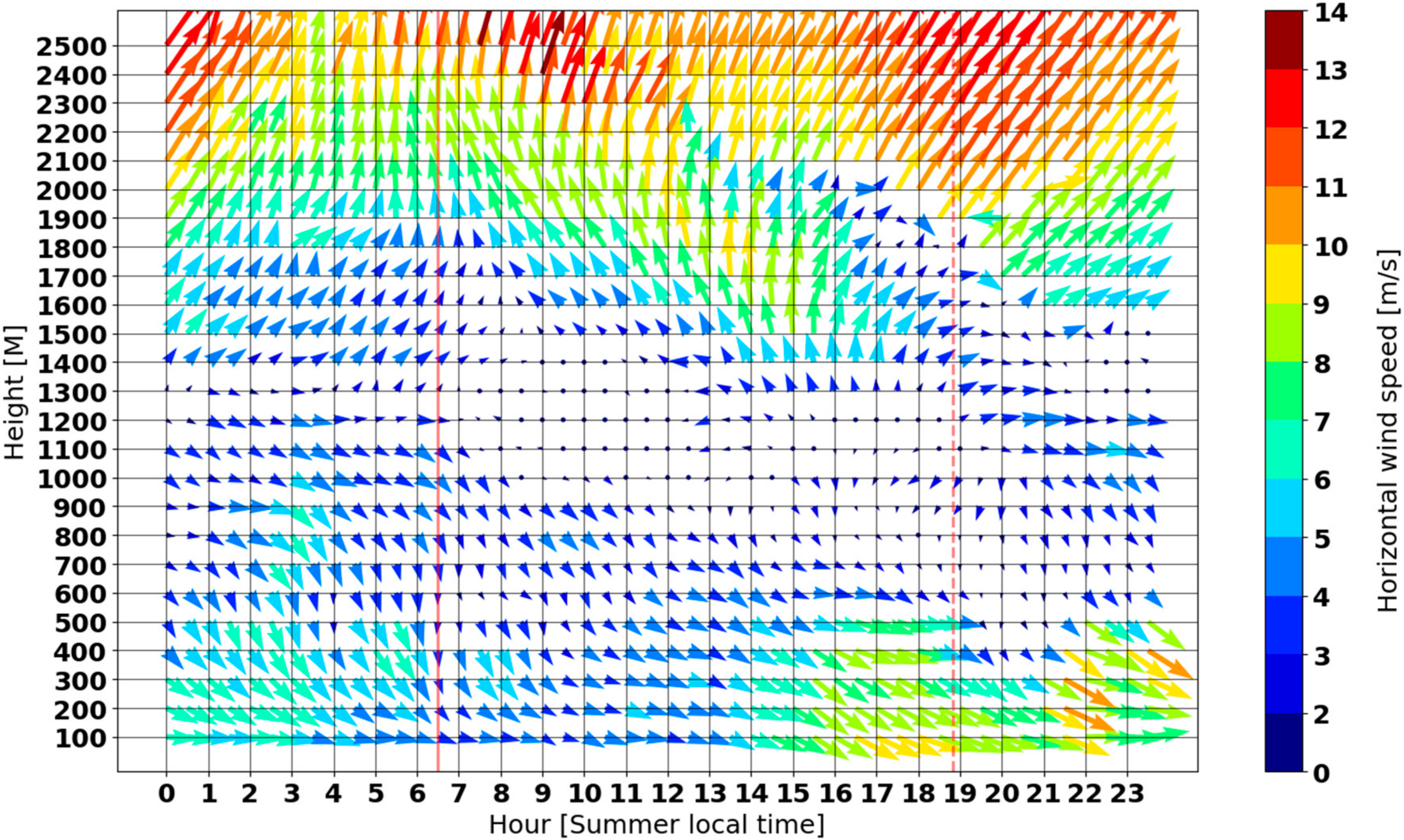
• The measurement technologies applied for the validation of the LiDAR are limited in their spatial coverage. Here, the validation procedure is enhanced by utilizing high resolution wind and temperature fields, produced by the meso-scale numerical weather prediction model WRF, which are compared to the LiDAR measurements.
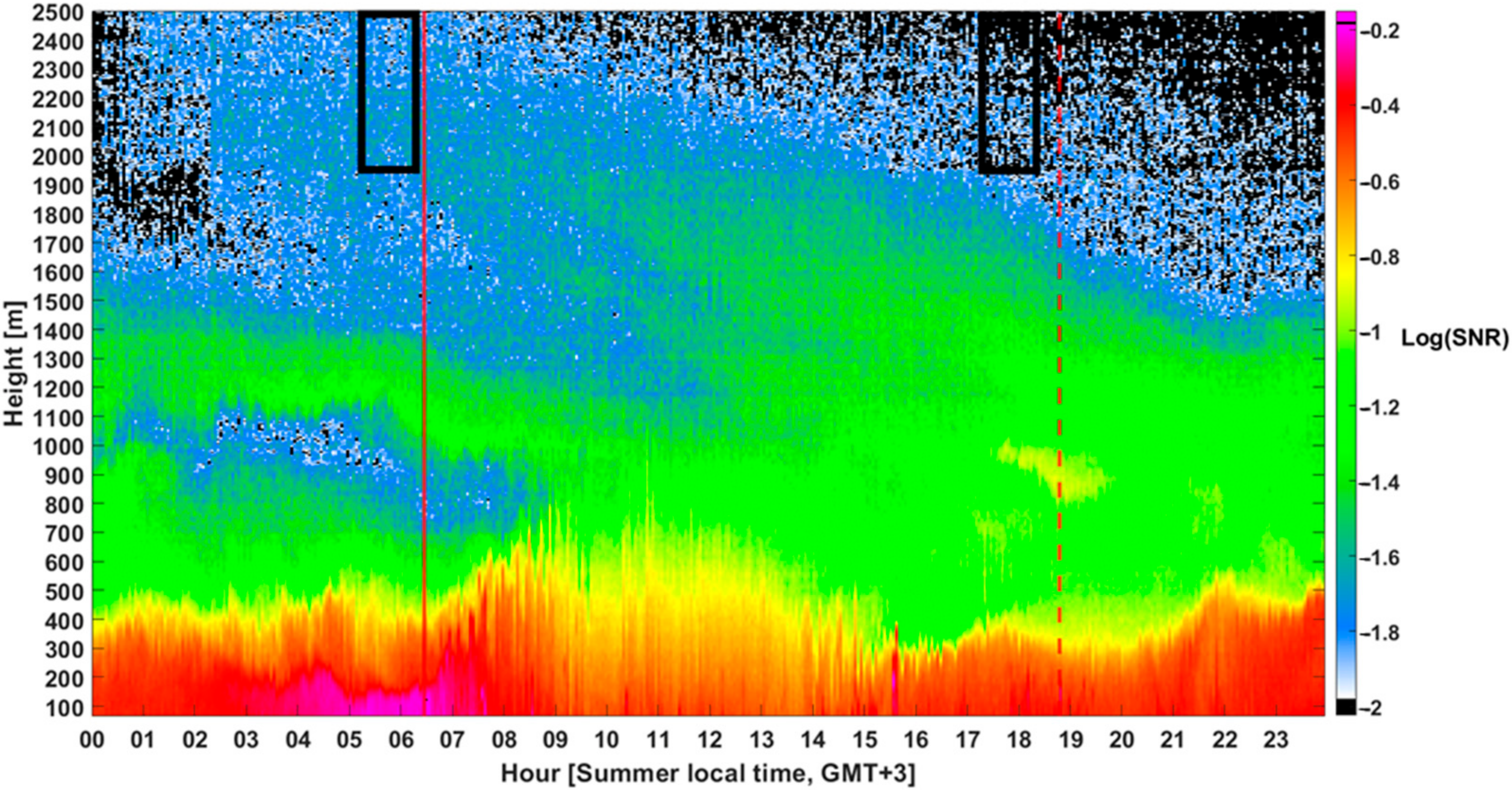
• A synergetic approach for the simultaneous application of LiDAR measurements and WRF predictions is shown. The LiDAR signal-to-noise ratio (SNR) depends upon the concentration of aerosols in the boundary layer, which can be too low for altitudes above the ABL. Model predictions also involve intrinsic uncertainty. Here, the atmospheric profile is studied using a combination of the two, which allows complementarity.

2. The Field Campaign: Location, Instrumentation and Models

Our field campaign took place in an open rural area near a fixed meteorological mast between the dates 13–15 September 2020. The location lies within the Jezreel valley, connecting the Mediterranean shores north of the Carmel ridge with the Jordan valley. the valley is bounded from south and north by low hills of up to 400 m above sea level. This topographic location leads to a channeling of westerly winds from the Mediterranean, and thus, the site is considerably affected by the sea breeze. The nearest town is located 8 km to the northwest, and the land use is mostly agricultural with low crops. The LiDAR, tethered balloon, and radiosonde launching point were located 550 m from the mast, and 29 m lower than its ground level, see site map in Figure 1. The site height is 88 m above sea level.

The Israel summer is characterized by persistence of synoptic weather patterns and by Mediterranean sea-land breeze development in the mesoscale [26,27]. During the summer (extending from June to September, included), the so-called Persian trough is the dominating synoptic regime at the surface characterized by north-westerly to westerly flow that is superimposed on Mediterranean sea breeze during daytime [28,29]. At upper levels subsidence dominates leading to the characteristic Mediterranean climate during the summer, exempt of precipitation [30]. Our measurements took place under Persian trough conditions according to reanalysis maps from ERA5 [31] and the development of the Mediterranean sea breeze. Therefore, insights from these measurements period are representative of the entire summer season.

The four wind measurement instruments are shown in Figure 2 and described in the following. It should be noted that, except for the LiDAR, all instruments measure only the horizontal wind components.

The source of atmospheric aerosols needed for LiDAR backscatter varies with height and wind direction. Westerly winds from the sea carry particulate matter (PM) from anthropogenic sources (industry and mobile) found in the Haifa metropolitan area and salt aerosol from sea spray. Dust of local and meso-scale sources can also be found [32].

2.1. Halo-Photonics StreamLine XR Doppler LiDAR

The StreamLine XR, Figure 2a, is a Doppler LiDAR system with a pulse length of 310 ns associated with a maximal resolution of 1.5 m along LOS. The LiDAR has a full scan range, from the horizon to the zenith operated with mirrors. The maximum range of this specific Lidar due to physical and processing limitations is ~12 km, though at large elevation angles the range will be limited to ~1–3 km due to insufficient aerosol concentration aloft, which is needed for backscatter of the signal.

Table 2. StreamLine XR LiDAR technical specifications.

Specification	Value
Pulse sampling frequency	100 MHz
Laser Wavelength	1550 nm
Laser Rap. Rate	10 KHz
Laser pulse length (FWHM)	310 ns
Output power (average)	400 mW
Average beam opening	60 $\mathsf{\mu }$rad
Scanner Elevation range	−3°–+90°
Scanner angle resolution	0.2 mRad
Scanner angular speed	1020 mRad/s
Wind velocity range	$38 {\mathrm{ms}}^{-1}$
Wind velocity precision	$0.04 {\mathrm{ms}}^{-1}$
Minimal range for measurements	30–40 m
Maximal range for measurements	6000–12,000 m
Range resolution System Dimensions in m (W × L × H)	1.5 m 0.6 m × 0.5 m × 0.4 m

presents the physical attributes of this system.

2.2. Tethered Balloon

The Vaisala Tethered balloon system, see Figure 2b, consisted of a variable number (2–5) of TTS111 tetheresondes mounted to the cable anchoring the balloon. The tetheresondes include a cup anemometer, which measures wind speed, a vane measuring wind direction, and sensors measuring altitude, pressure, and temperature with a variable sampling time ranging from 10 s to 1 min per each sonde. During this study, the tetheresondes were mounted between 150 m to 900 m in increments of about 100 m. Data availability was partial due to communication problems. Hence, the acquired data included 2–5 tetheresondes at a time. The resolution of wind speed measurements is 0.1 ms⁻¹, minimal wind velocity is about 0.5 ms⁻¹ and the uncertainty of wind speed is around 0.2 ms⁻¹ [33,34]. The resolution of direction measurement is 1°. It is important to note that some uncertainty, uncharacterized by the technical specifications of the tetheresonde itself, stems from the fact the cable typically forms a slanted orientation due to the wind force exerted on the balloon. Thus, the tethersondes are not necessarily located right above the LiDAR. Considering an operational wind speed threshold of 12 ms⁻¹ and the operation heights not higher than 1000 m the horizontal drift is no more than 150 m.

2.3. Meteorological Mast

The meteorological mast, shown in Figure 2c, is owned by “EDF Renewables Israel” and “Blue Sky Energy” and operated by “NextCom”. Two pairs of cup anemometers (Thies Clima, “First Class” Advanced, part num. 4.3351.00.100 [35]) mounted on perpendicular horizontal booms measure horizontal wind speed at heights of 60 and 80 m above the ground (89 m and 109 m above the LiDAR’s location). Wind direction is measured by Two vane sensors (Thies Clima, “First Class” Advanced, part num. 4.3351.10.400 [35]) at 45 m and 75 m (74 m and 104 m above LiDAR’s location). The uncertainty of velocity measurements is 1% of the measured value (minimum of 0.2 ms⁻¹) and the starting threshold is 0.3 ms⁻¹. For the campaign purposes, 10 min averaged data were used. The mutual difference between the cup anemometers in a pair was lower than 0.2 ms⁻¹ and did not exceed 2.5% of the pair average. Thus, the pair average was regarded for the comparison.

2.4. Radiosondes

A total of 18 Radiosondes (M10 Meteomodem, Ury, France)(see Figure 2d) were launched during the campaign, usually four launches throughout the day and two during the night. The Radiosondes provided the meteorological parameters of the atmosphere, including temperature, pressure, and relative humidity up to altitudes of ~30 km for about an hour and a half. The sampling frequency is 1 s and the balloon vertical speed is 4–6 ms⁻¹. The accuracy of velocity measurements is 0.15 ms⁻¹ and the resolution of direction is 1°. For the temperature and the relative humidity, accuracy is 0.3 °C and 3%, respectively. Typical radiosonde trajectories are seen in Appendix A in Figure A2.

2.5. WRF Model

The WRF model is one of the most advanced mesoscale numerical weather prediction models available, designed to serve both operational forecasting and atmospheric research. Prognostic variables include horizontal and vertical wind components, various microphysical quantities, potential temperature, geopotential, and surface pressure. WRF has a nesting grid capability that allows zooming into a sub-region with high horizontal resolution by generating a series of higher resolution child grids within coarser parent grids. WRF includes a complete suite of physics schemes that account for the important atmospheric and land-surface physics. Several different formulations are available for each of these schemes, used to define the model topography and other static surface fields. For a complete description of the WRF modeling system, see, e.g., ref. [36].

We use the WRF model (version 4.0) with the Advanced Research WRF (ARW) solver for the simulations. We ran a two-way 3-nested domains configuration. The three domains with horizontal grid sizes of 13.5, 4.5 and 1.5 km are shown in Appendix A, Figure A1. The model configuration including vertical grid, physical parameterizations, numerical options and initialization time was chosen as in the reference runs in [37]. The ERA5 global reanalysis [31] was used for initial and boundary conditions.

WRF model has been widely used to simulate and forecast the boundary layer conditions and in particular the vertical profile of the horizontal wind [37,38,39,40]. In all of the cited cases the model reproduced the shape of horizontal wind profile satisfactorily when compared to observations. In particular, Fovell and Gallagher [40] published a thorough verification of short-term WRF-forecasts profiles of horizontal winds within the PBL up to 1 km above ground level using radiosoundings over the continental USA. Their results show WRF wind-speed positive biases along the profile within the range ~0.5–1.2 ms⁻¹.

3. Methods

3.1. Comparison of Doppler LiDAR Relative to Other Measurement Techniques

The Doppler LiDAR StreamLine XR was operated in three scan methods. To allow flexibility, the scan methods presented in this work were three procedures that were written in-house. These procedures were a “stare” scan in the vertical direction, a VAD scan with 24 beams and a DBS scan with 3 beams: vertical LOS, north LOS with a fixed elevation and east LOS with the same elevation. To study the sensitivity to elevation angle, scans were operated in two elevation angles of 60° and 80°.

The LiDAR was configured to operate with a gate length of 12 points (a corresponding gate length of 18 m) with an overlapping sequence that produced a measurement spatial resolution of 1.5 m along LOS. Above the mixing layer, the returned signal diminishes quickly due to the rapid decline of aerosol concentration. The in-situ measurements of other instrumentation were conducted at altitudes under 1000 m. For this reason, and as a consequence of the LiDAR’s limitations in measuring in low aerosol density, the number of gates was limited to 3840 with an overlapping 18-m gate length, resulting in a maximum altitude measurement of 5764 m. The radial velocity is measured by averaging 10,000 pulses per ray.

The advised SNR+1 threshold is ~1.015. However, in order to increase data availability, we applied a technique [1,3,41,42], which relates the SNR to its measurement precision, following which SNR threshold value of 0.0095 was selected. Details of the process are described in Appendix C.

A scanning operation procedure was built to perform six different scans automatically. This program was operated continuously with a cycle time of ~5 min, as follows:

• A DBS scan at 60° with 3 beams and a duration of 14 s. (referred to as “DBS 60”).
• A VAD scan at 60° with 24 beams and a duration of 36 s. (referred to as “VAD 60”).
• A DBS scan at 80° with 3 beams and a duration of 14 s (referred to as “DBS 80”).
• A VAD scan at 80° with 24 beams and a duration of 36 s (referred to as “VAD 80”).
• A VAD scan at 75° with 6 beams and a duration of 6 s.
• A stare scan at 90° and processing with a duration of ~1:30 min.

Extraction of wind components u, v, and w was performed similarly to the methods presented in [18] and [1] (Our methods and equations are presented in Appendix B). The extraction is performed under the assumption the winds are uniform along each horizontal cross section of the scan volume. In order to get an estimation of wind uniformity, each wind speed measurement was compared to a sinusoidal wave (see the method presented by Smalikho and Banakh [43]), where high correlation indicates wind uniformity. It is important to note that this check is performed with the assumption that the vertical component contribution is negligible.

The different instruments differ in their sampling rates. Therefore, an averaging time interval is introduced in order to have a common time base for comparison. A 30-min averaging time interval was selected, which compromises an adequate number of samples in each interval with the requirement of flow persistence.

Heights of LiDAR data for comparison were selected to optimally match the location of the different in-situ sensors. This is not trivial for the tethered balloon sensors, which do not, in general, keep a constant altitude. Ascent and descent of the balloon takes time during which the height of the sensors keeps changing. Furthermore, even in its full rise position, the balloon drifts in the wind direction, which affects the orientation of the cable and alters the heights of the sensors. To enable comparison to LiDAR data, the heights of each sensor were averaged over each 30 min time period to yield a single representative height. For cases in which the absolute median deviation of a sensor height throughout the averaging period was larger than 15 m, the measurements for that period were disregarded.

Agreement of LiDAR observations with each of the corresponding instruments was assessed differently for wind speed and for wind direction. In the latter case, the agreement was statistically expressed by calculating the average difference (Bias)

$$\mathrm{Bias}=\frac{1}{\mathrm{N}}{{\displaystyle \sum }}_{\mathrm{i}=1}^{\mathrm{N}}{\mathrm{d}}_{\mathrm{i}},$$

(1)

and its standard deviation (STD)

$$\mathrm{STD}=\sqrt{\frac{1}{\mathrm{N}}{{\displaystyle \sum }}_{\mathrm{i}=1}^{\mathrm{N}}{({\mathrm{d}}_{\mathrm{i}}-\mathrm{Bias})}^2}.$$

(2)

${\mathrm{d}}_{\mathrm{i}}={\mathrm{L}}_{\mathrm{i}}-{\mathrm{C}}_{\mathrm{i}}$ is the mutual difference for time period $\mathrm{i}$ between the wind direction measured by the LiDAR, ${\mathrm{L}}_{\mathrm{i}}$ and measured by the corresponding instrument, ${\mathrm{C}}_{\mathrm{i}}$. Circular periodicity is taken into account by altering ${\mathrm{d}}_{\mathrm{i}}$ according to

$${\mathrm{d}}_{\mathrm{i}}=\{\begin{array}{cc}{\mathrm{d}}_{\mathrm{i}}-360\hfill & {\mathrm{d}}_{\mathrm{i}}>180\\ {\mathrm{d}}_{\mathrm{i}}+360\hfill & {\mathrm{d}}_{\mathrm{i}}<-180\end{array},$$

(3)

For wind speed, agreement was statistically estimated by goodness of fit (R²) and by the bias of a linear regression.

3.2. ABL Structure Analysis

Heat, momentum, moisture and PM are vertically transported across the boundary layer by means of turbulence which is typically induced by velocity and temperature gradients between the surface and the adjacent atmospheric flow. The mixed layer (ML) is defined as the lower part of the ABL, in which active turbulence leads to efficient vertical mixing and redistribution. The ML height (MLH) which is the top boundary of the ML, is characterized by a decrease in turbulence intensity and PM concentration [44]. Estimating the MLH and studying its dynamics is important for the study of atmospheric pollutants which are diluted more efficiently as the ML deepens [45].

Often, typically during daytime, the MLH is related to an elevated temperature inversion layer, inhibiting vertical motion and turbulence. By inhibiting vertical momentum exchange, an inversion layer decouples different layers in the atmosphere, potentially allowing the coexistence of different flow regimes in each layer.

LiDAR measurements are used to assess the MLH and the existence of temperature inversions in different ways:

• The 30 min standard deviation of vertical velocities as a function of height, ${\sigma }_w\left(z\right)$, gives a direct indication of vertical turbulent intensity [14,15]. Following Park et al. [15], the height where ${\sigma }_w\left(z\right)$ drops below 0.2 ms⁻¹ is identified as the MLH.
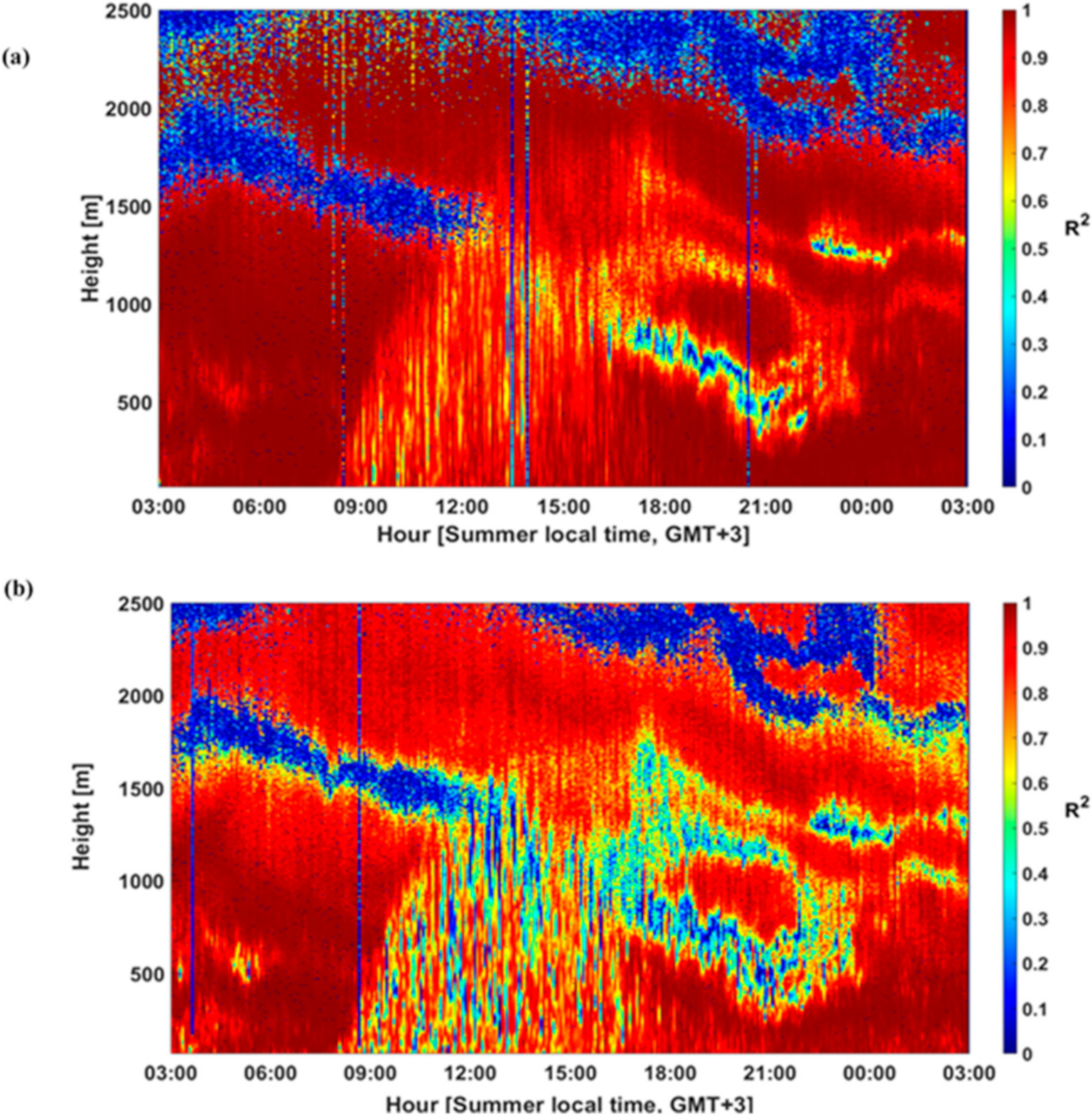
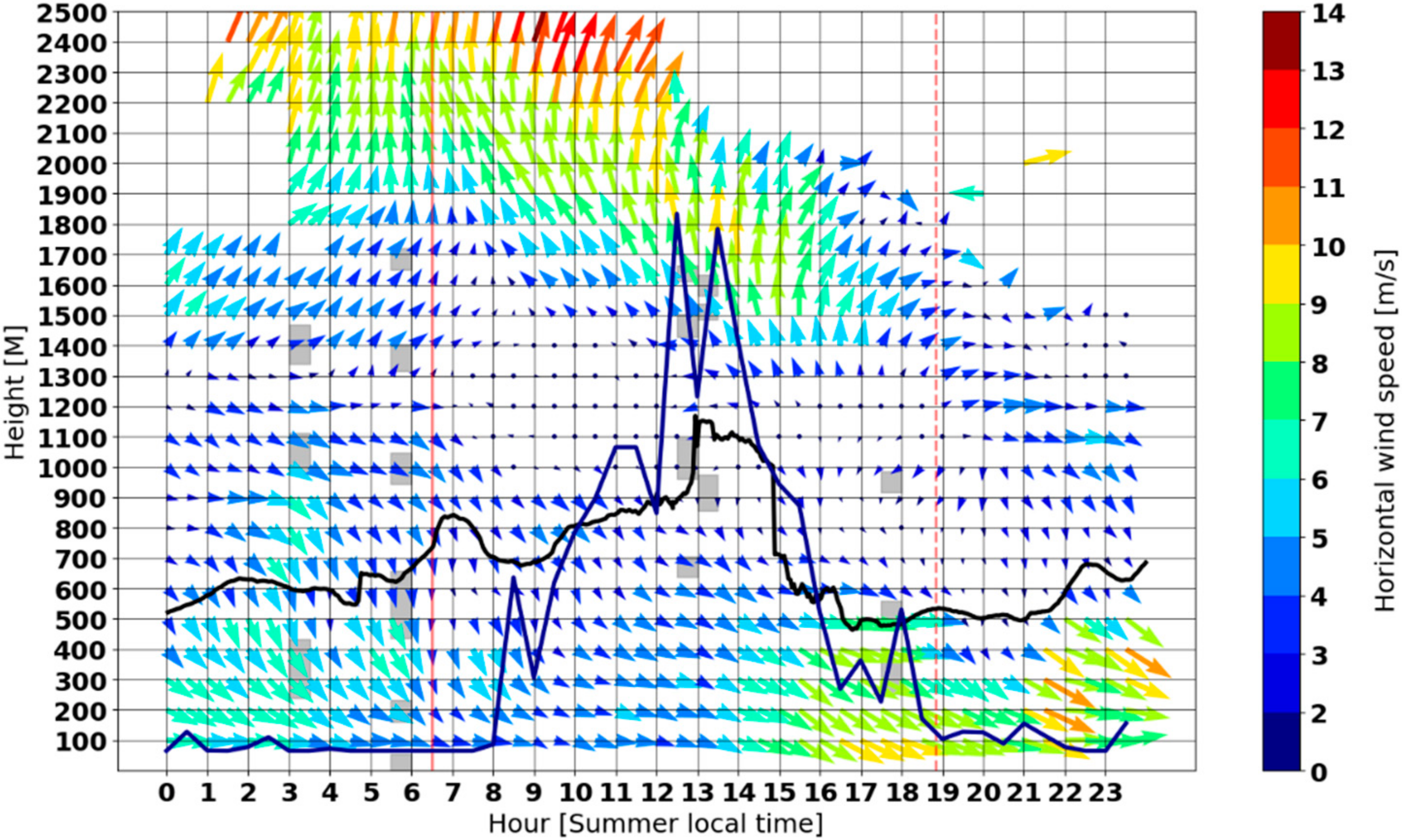
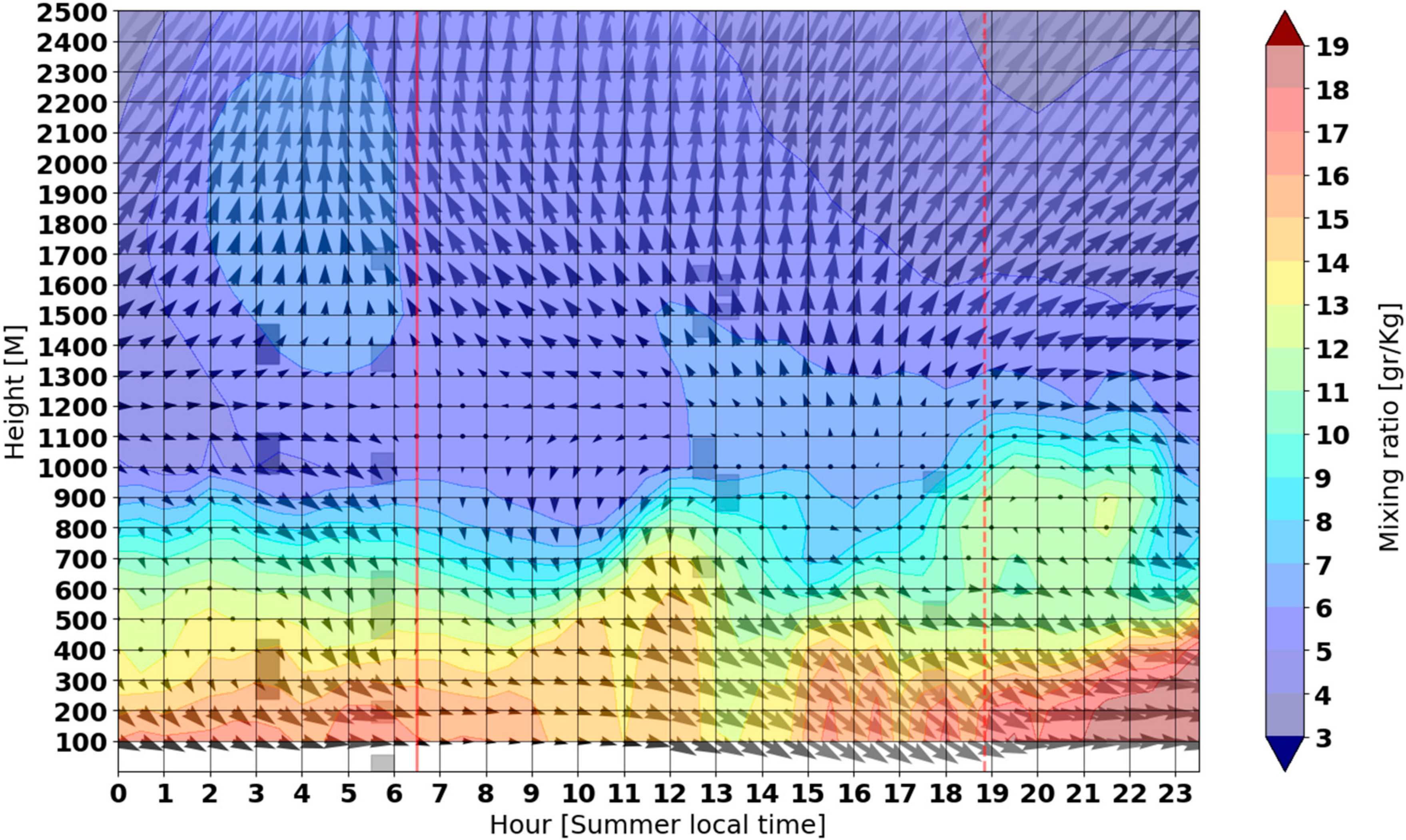
• The distribution of PM concentration along the vertical profile indicates the ML depth. The boundary between the ML and the free atmosphere aloft is typically noticeable as a transition zone in which a relatively large negative vertical gradient in the PM concentration prevails [46]. Above this transition zone, the PM concentration is considerably lower than below it. Multiple algorithms have been proposed to quantitatively detect and extract the MLH from attenuated backscatter data [47]. Here, we use the wavelet method [14,15,46,48] applying convolution of Haar function over the attenuated backscatter profile. This results in a function in which sharp negative (positive) gradients are expressed as peaks (deeps). The position of these peaks indicates the center of the transition zone, their magnitude is associated with the gradient strength, and their width indicates the depth of the transition zone. When multiple peaks are detected, the strongest magnitude of the two is selected. The top limit of the transition zone is defined as the MLH.
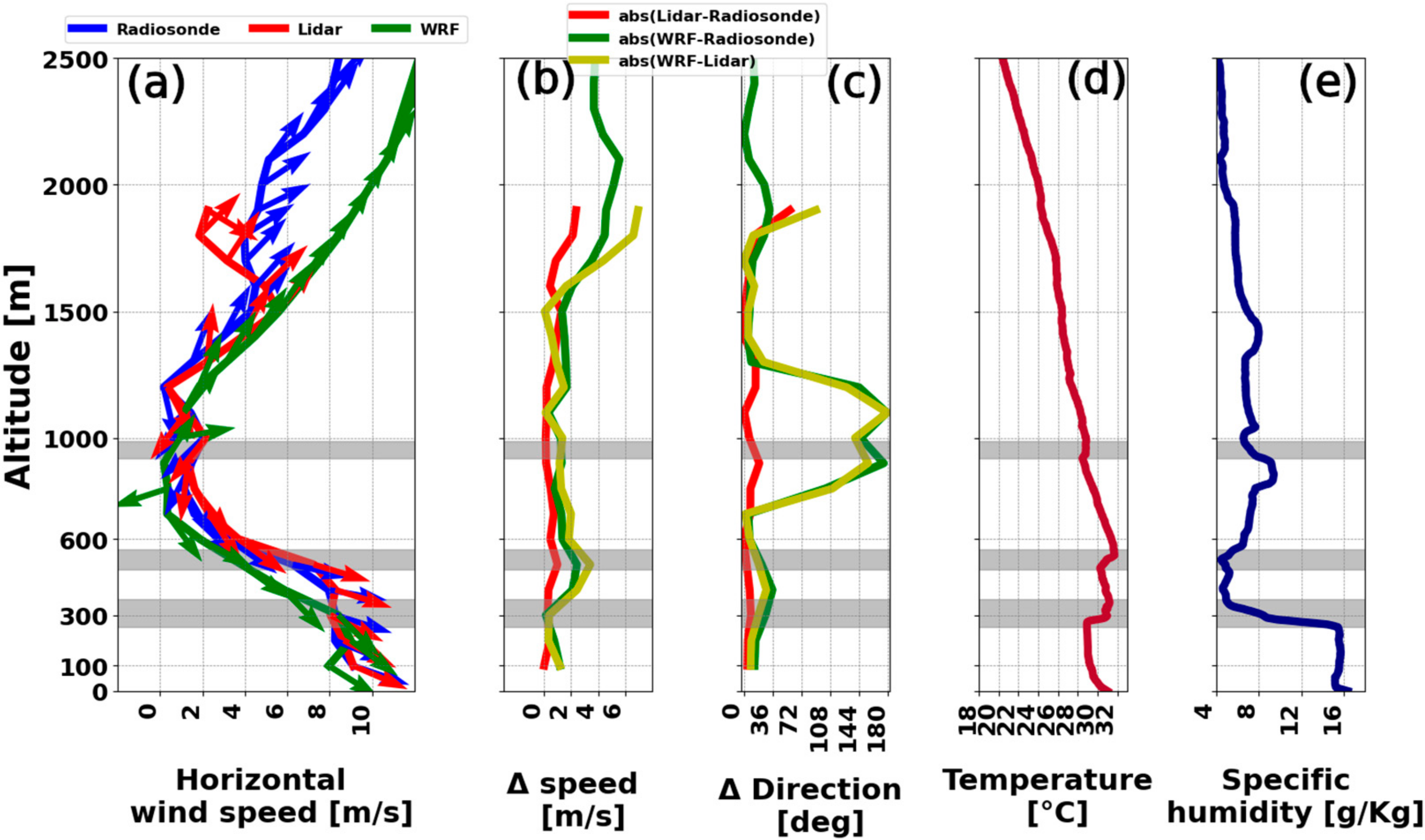
• Temperature inversions can be indirectly identified from LiDAR horizontal wind measurements. The inhibition of vertical turbulent momentum transfer, associated with an inversion layer, may allow strong direction and speed gradients.

Temperature inversion layers detected by radiosonde observations were identified and their locations were cross compared with the estimated MLH. Also, the impact of the inversion layers on vertical gradients along the measured wind profile was qualitatively assessed.

WRF forecasts for the period of interest were used to replace measurement gaps for elevations and times where SNR was lower than the selected threshold (see Section 3.1). The elevation for which WRF data was used remains above 1500 m and changes diurnally. This elevation is part of the free atmosphere, above the boundary layer. On one hand, this is the reason why aerosol concentration in these regions is not always sufficient to sustain large SNR values. On the other hand, WRF generally performs better for these heights, where the wind is less affected by topography and surface-flow interactions which may not be sufficiently resolved [49]. Thus, in this work, the potential of using WRF data and LiDAR observations synergistically to produce a combined product is preliminarily examined. WRF data is also inspected against radiosonde and LiDAR observations for assessing the ability of WRF to reproduce the observed boundary layer structure.

4. Results

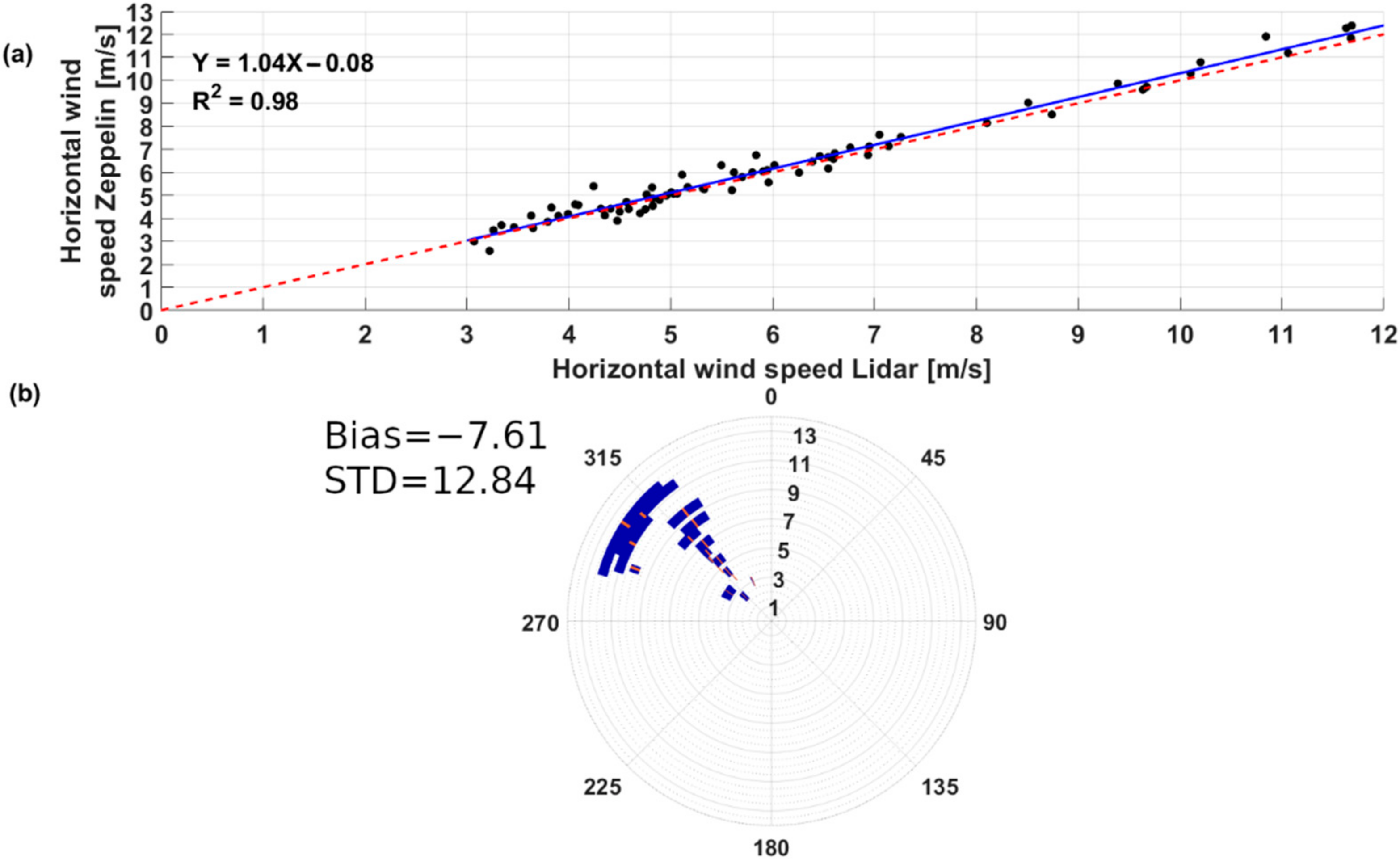
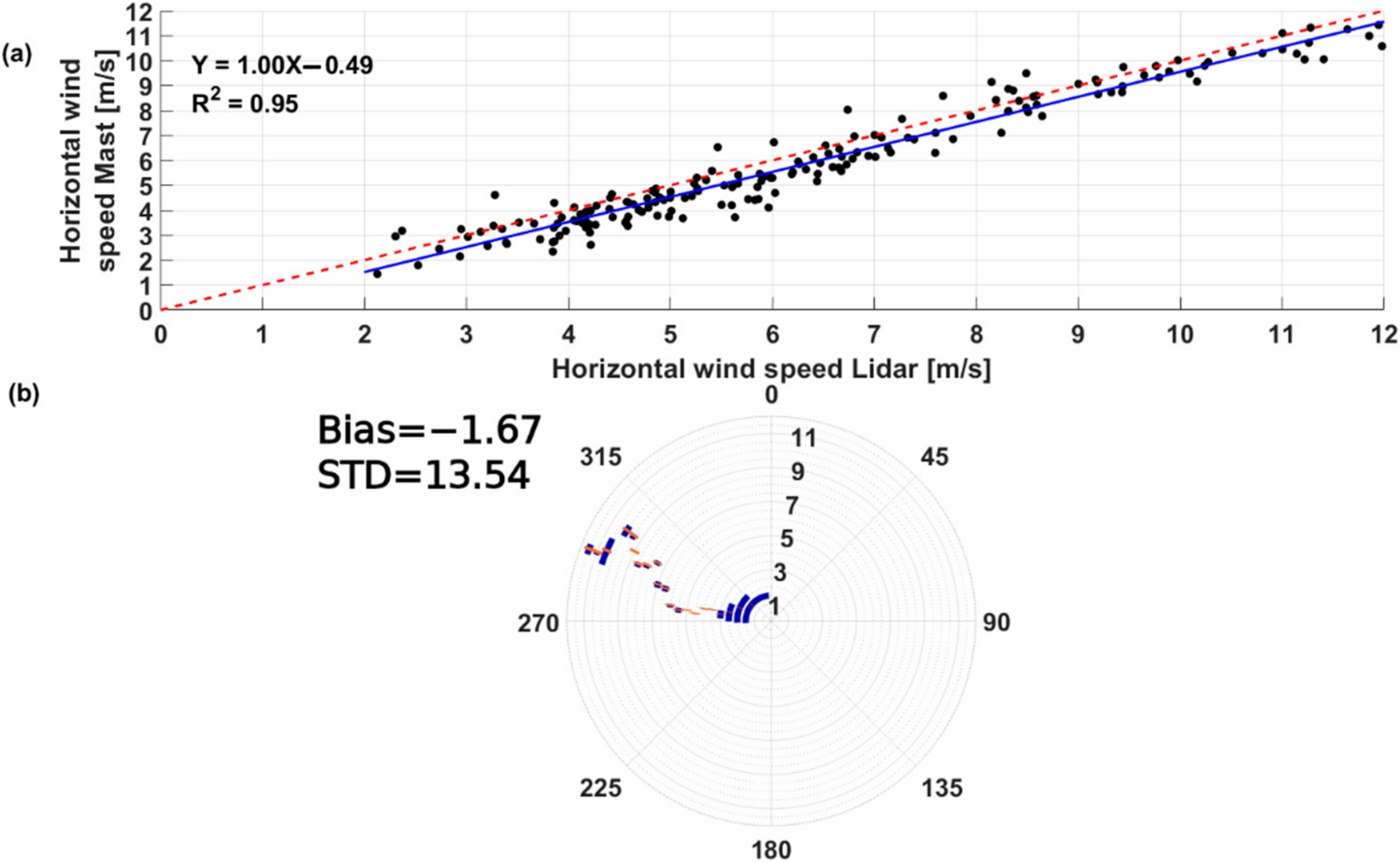
4.1. Statistical Cross-Validation of LiDAR Observations

Comparison of the LiDAR observations to the tethered balloon, mast, and free radiosondes was performed separately for each of the scan modes VAD 60, VAD 80, DBS 60, and DBS 80. For very weak winds (<2 ms⁻¹), data were discarded.

Table 3. Distribution of heights for tetheresonde data.

Height (m)	50–200	200–350	250–500	500–650	650–800	800–950
Percentage (%)	12	27	31	14	14	2

presents the distribution of tetheresondes data between different heights.

Figure 3a shows, as an example, a scatter plot comparing wind speed observations between the LiDAR VAD 60 scan and the tethered balloon. A dashed red curve corresponds to an ideal agreement between the two data sets, which is closely matched (R² = 0.98, bias of −0.08 ms⁻¹) by a linear best fit (equation embedded in the figure), shown by a solid blue curve.

Figure 3b presents the corresponding comparison for wind direction. The angular extent of each arc corresponds to the average difference of wind directions, and its marked center is in the average wind direction. To depict sensitivity to wind speeds, the calculation is done separately for different wind speeds, shown by the radial position of each arc. Bias and STD values (Equations (1) and (2)) are also presented. The comparison presented in Figure 3 is based on 74 measurement points (each point is an average of 9–12 LiDAR profiles).

A similar comparison between the LiDAR DBS 60 scan and the mast sensors is presented in Figure 4. Good agreement in the horizontal wind speed is observed, with R² = 0.95 and a bias of −0.49 ms⁻¹. The wind direction standard deviation is 13.54° and the bias is −1.67°, with a higher difference in the wind direction at lower horizontal wind speeds, a trend that is seen in all the scans and mast comparisons. The comparison presented in Figure 4 is based on 96 averaged profiles resulting in 192 measurement points (likewise, each point is an average of 9–12 LiDAR profiles).

A summary of the comparison between all LiDAR measurements versus tethered balloon and mast observations is given in

Table 4. Summary of comparison between LiDAR scans and other instruments, the number of averaged (30 min averaging time) measurement points used for the comparison of each instrument is specified.

	DBS 60	DBS 80	VAD 60	VAD 80
LiDAR vs. tethered balloon system (74 measurement points)	Correlation of horizontal wind speed
	${\mathrm{R}}^2=0.95$ $\mathrm{Bias}=0.36$ $\mathrm{Rmse}=0.51$	${\mathrm{R}}^2=0.92$ $\mathrm{Bias}=0.33$ $\mathrm{Rmse}=0.68$	${\mathrm{R}}^2=0.98$ $\mathrm{Bias}=0.08$ $\mathrm{Rmse}=0.36$	${\mathrm{R}}^2=0.90$ $\mathrm{Bias}=0.46$ $\mathrm{Rmse}=0.77$
	Correlation of horizontal wind direction
	$\mathrm{STD}=14.28$ $\mathrm{Bias}=-7.4$	$\mathrm{STD}=18.68$ $\mathrm{Bias}=-6.94$	$\mathrm{STD}=12.84$ $\mathrm{Bias}=-7.61$	$\mathrm{STD}=15.57$ $\mathrm{Bias}=-7.13$
LiDAR vs. mast (192 measurement points)	Correlation of horizontal wind speed
	${\mathrm{R}}^2=0.95$ $\mathrm{Bias}=-0.49$ $\mathrm{Rmse}=0.57$	${\mathrm{R}}^2=0.90$ $\mathrm{Bias}=-0.17$ $\mathrm{Rmse}=0.78$	${\mathrm{R}}^2=0.94$ $\mathrm{Bias}=-0.33$ $\mathrm{Rmse}=0.61$	${\mathrm{R}}^2=0.92$ $\mathrm{Bias}=0.38$ $\mathrm{Rmse}=0.71$
	Correlation of horizontal wind direction
	$\mathrm{STD}=13.54$ $\mathrm{Bias}=-1.67$	$\mathrm{STD}=16.69$ $\mathrm{Bias}=0.16$	$\mathrm{STD}=13.76$ $\mathrm{Bias}=-2.2$	$\mathrm{STD}=13.48$ $\mathrm{Bias}=-3.48$

. Regardless of the scan mode, horizontal wind speed agreement between LiDAR and balloon observations is good, with R² ≥ 0.90 and bias ≤ 0.46 ms⁻¹, respectively. STD for the wind direction is ≤18.68° and the absolute bias ≤ 7.61°. The agreement of LiDAR and mast observations is also good with R² ≥ 0.90 and an absolute bias ≤ 0.49 ms⁻¹ for wind speed. The wind direction STD is ≤16.69° and the absolute bias is ≤3.48°. For both the mast and balloon comparisons, 60° elevation scans perform slightly better than 80° scans. VAD scans seem slightly better than DBS scans for tethered balloon comparison, and vice versa for lower altitude mast comparison.

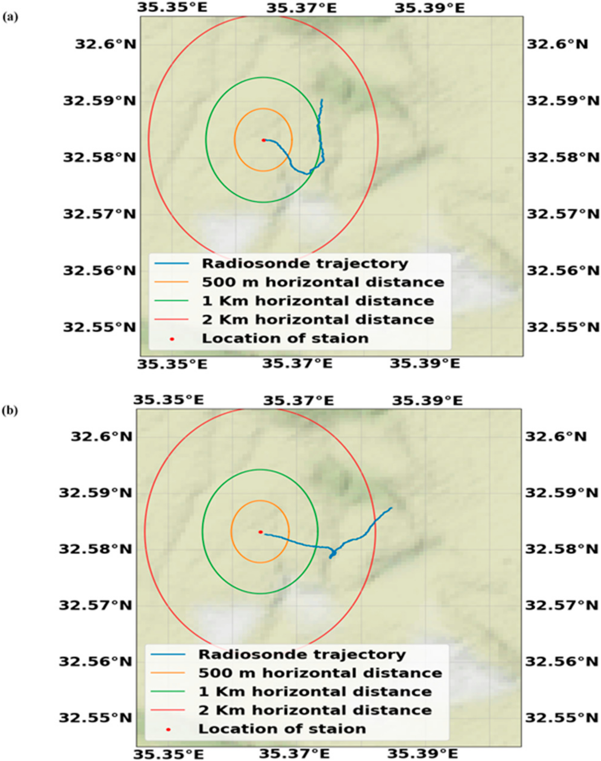
4.2. Spatial Uniformity

It is of interest to quantitatively explore the origin of difference between scans with 60 and 80 elevation angles. This can be done by assessing wind uniformity along horizontal cross sections within the cone-shaped volume formed by VAD scans. Quantifying uniformity can be done by applying sine wave fitting [18]. Consider a VAD scan with ${\mathrm{V}}_{\mathrm{i}}$ the radial velocity measurement $\mathrm{i}$ for the azimuthal direction ${\mathsf{\theta }}_{\mathrm{i}}$. A least squares best fit sine function

$${\mathrm{v}}_{\mathrm{i}}=\mathrm{Asin}\left({\mathsf{\theta }}_{\mathrm{i}}+\mathrm{B}\right)+\mathrm{C},$$

(4)

is calculated, and the measure for wind uniformity is thus estimated by the R² goodness of fit, i.e.,

$${\mathrm{R}}^2=1-\frac{{{\displaystyle \sum }}_{\mathrm{i}}{({\mathrm{V}}_{\mathrm{i}}-{\mathrm{v}}_{\mathrm{i}})}^2}{{{\displaystyle \sum }}_{\mathrm{i}}{({\mathrm{V}}_{\mathrm{i}}-\overline{{\mathrm{V}}_{\mathrm{i}}})}^2},$$

(5)

Figure 5 shows R² values of sine-wave fitting for VAD 60 (a) and VAD 80 (b) scans. It is shown that a scan at 60° has more areas in the profile with higher R² values, compared to a scan at an angle of 80°. This means that a 60° scan better meets the horizontal wind uniformity assumption upon which wind component extraction is based. This conclusion is consistent with the above observation of improved performance for VAD scanning at 60° over corresponding scans with 80° elevation angle.

A note regarding the counter intuitiveness of this result should be made. One could have expected that higher elevation angles, which reduce the scanning volume, would improve spatial homogeneity yielding higher R² values. However, a side effect of narrowing the cone-shaped scan volume is the enhanced introduction of vertical velocity into the measured radial velocity. Unlike the horizontal velocity which spatially fluctuates by no more than a few tens of percent (and much less for strong winds), the vertical wind can fluctuate drastically and even change its direction (upward/downward) between different locations along the scan cross section. Therefore, introducing more of the vertical component actually degrades spatial homogeneity, leading to lower R² values for the 80° angle.

Inclusion of vertical wind into the extraction algorithm affects the wind uniformity assumption differently for different boundary layer static stabilities. As evident from Figure 5, lower R² values are attained from 9:00 to 18:00, for which boundary layer convective instability promotes enhanced vertical turbulence. Respectively, lowering of R² values for 80° angle scans is mostly pronounced for this time range.

4.3. Boundary Layer Structure Analysis

Aside from direct wind observations, LiDAR measurements may serve to analyze the boundary layer structure, including MLH identification and the indirect identification of temperature inversion layers, which decouple the profile into different layers characterized by different flow regimes. In the following section, the synergic use of LiDAR observation and WRF simulations for the analysis of boundary layer structure and features will be shown for a specific diurnal period.

An indication regarding boundary layer structure can be given by attenuated backscatter profiles. Figure 6 shows profiles of the attenuated backscatter ($\beta [{\mathrm{sr}}^{-1}{\mathrm{m}}^{-1}]$) for the day 15 September 2020. Blue and black curves mark the MLH as estimated using ${\sigma }_w$ and $\beta$-wavelet methods, respectively. High values of $\beta$ correspond to higher concentrations of scattering elements in the atmosphere, such as aerosols and hydrosols.

The profiles change throughout the period, exhibiting layers of high and low concentrations. The two MLH estimation shows agreement during most of the daytime hours, when the MLH and the elevated inversion layer coincide. During evening and night hours, ground inversion inhibits turbulence, and the ${\sigma }_w$-estimated MLH remains under the minimal LiDAR range most of the time. For these hours, a residual layer of PM persists above the ${\sigma }_w$-estimated MLH, which leads to a considerable difference between the MLH attained by the two methods.

Above the MLH, more layering can be (subjectively) observed. This is especially true for the late night and early morning (01:00–08:00), where a layer characterized by high backscatter signal can be identified roughly between the heights 100–1500 m. Persistence of concentration layering may suggest the existence of strong inversion layers, inhibiting vertical motion and decoupling adjacent layers.

Five radiosondes were launched in the period of interest. Elevation ranges along the profile which are characterized by positive temperature gradients monotonically persisting along more than 50 m are identified as inversion layers and are marked by grey shading in Figure 6. Some of the temperature inversion layers correspond to gradients in aerosol concentration. This is especially true for the inversion associated with MLH and for the additional inversion layers which decouple the aerosol layer in the late night and early morning hours between the heights of 1000 and 1500 m. The identification of inversion layers is thus indirectly expressed by backscatter LiDAR observations.

The relation between the observed temperature inversions and the algorithmically detected MLH is worth noting. In all launches except for the first one, the MLH detected by the ${\sigma }_w$ method corresponds to one of the inversion layers. Moreover, for the three last launches, the different MLH estimations attained by the two methods correspond to two different inversion layers.

In areas where inversion layers inhibit vertical airflow, momentum fluxes are reduced, and consequently, strong wind speed and direction gradients may be observed along the profile. Figure 7 presents that phenomenon by showing the horizontal-wind profile measured by the LiDAR. The direction of the arrows depicts the horizontal wind direction (arrow pointing down corresponds to northerly wind, right-pointing corresponds to west, etc.), and their length and color correspond to the wind speed. Where SNR data were not sufficiently high, no arrow is displayed. Inversion layers, as identified by radiosonde observations, are shown by grey shading. It can be seen that in some cases the inversion layers are associated with wind speed or direction gradients.

By comparing Figure 6 and Figure 7, a better understanding of the profile structure is obtained. The profile can be divided into 3 layers: 1. A low altitude layer with western northerly winds which persist throughout the diurnal period. 2. An intermediate layer characterized by very weak winds which changes in thickness throughout the day. 3. An upper layer with strong south western to south eastern winds. A considerably deep layer characterized by sub-threshold SNR values can be seen in the upper right corner of Figure 7. The lacking data starts at around 13:00 at 2500 m altitude, and gradually thickens to a layer of ~1400–2500 m at the end of the diurnal period. As Figure 6 reveals, this missing part of the graph is associated with low attenuated backscattering signal, leading to low SNR values.

To gain further insight into the measured wind profiles, the SNR values should be evaluated. The log of the SNR values for the considered period is color coded in Figure 8. The evening profiles above ~2000 m exhibit extremely low SNR values.

A more complete picture can be attained by using WRF model forecasts. Figure 9 presents the corresponding horizontal wind profiles that were produced by the WRF model. Shaded grey blocks marking the inversion layers extracted from radiosonde data, and shaded red areas correspond to inversions extracted from the forecasted temperature profiles, using the same criteria.

Features of the boundary layer are well obtained, including the division to 3 layers. However, the resolution of the WRF vertical grid at heights of hundreds of meters is around 100 m, and as a result, the temperature gradients creating the inversion layers are not correctly resolved and the modelled inversion layers are considerably coarser. During early night hours (20:00 on), the emergence of an elevated low-level jet around 300–400 m above ground is witnessed both in the LiDAR observations and in the model prediction.

The good agreement between the wind profiles observed by the LiDAR and the simulated profiles may serve to support utilization of the modeled wind in areas where the LiDAR SNR is too low to obtain valid observations. Figure 10 shows a combined product in which missing LiDAR observations are filled using WRF data. The prevailing wind aloft, which the LiDAR fails to observe, is the synoptic south westerly wind, which persists with little diurnal variation.

The synergic use of LiDAR observation with WRF simulations can be further supported by the analysis of radiosonde data. Figure 11 and Figure 12 present radiosonde measurements, LiDAR wind profile, and the corresponding WRF simulations during 5:30–6:00 and 17:00–18:00, respectively. These two times represent conditions of large and poor SNR, respectively, for altitudes above 2000 m (see black rectangles in Figure 8 above). Panel a in both figures display the horizontal-wind speed (horizontal position of arrows) and direction (constant-size vectors) as a function of height (vertical axis). Radiosonde, LiDAR, and WRF data are displayed by blue, red, and green curves, respectively. Panels b and c in both figures depict the absolute differences of speed (b) and direction (c) between the LiDAR, radiosonde, and model data.

For the first case (Figure 11a), good agreement between radiosonde and LiDAR profiles is evident, with WRF profile underestimating speed around the altitudes 600 m and 1400 m. These altitudes correspond to inversion layers (shaded) and are likely caused by discrepancies in the inversion heights forecasted by the model. For the afternoon case, (Figure 12a) wind profiles obtained by the LiDAR and by radiosonde exhibit good agreement under 1500 m, with WRF slightly overestimating wind speed at 1400 m and slightly underestimating it around 500 m. Above 1500 m, for which the LiDAR data is invalid, WRF satisfactorily replicates the wind direction measured by the radiosonde, although with a considerable overestimation of wind speed compared to literature known biases (see Section 2.5).

Radiosonde observations can be further utilized to validate the analysis of the diurnal boundary layer structure. Radiosonde temperature and specific humidity profiles (Figure 11 and Figure 12, panels d and e) reveal the locations and extent of multiple inversion layers (shaded in the figure) which decouple adjacent layers. For the early morning case (Figure 11), an inversion layer around 600 m buffers a near surface layer with high moisture content, and a dryer layer extending up to 1000 m. Two additional inversion layers allow the formation of another high humidity layer between 1000 m and 1300 m. The suppression of momentum exchange associated with inversion layers leads to the expression of these layers though the wind profile (panel a). The boundary layer is divided into layers with north-westerly winds (ground to 1000 m), western winds (1000–1300 m), and south westerly winds aloft.

The evening radiosonde observations (Figure 12) can be similarly analyzed. Here, two low inversion layers at 300 m and 500 m, and a subsequent one at about 1000 m, divide the boundary layer into a very moist shallow layer up to 300 m, followed by a much dryer layer up to 500 m, another layer between 600 and 1000 m, where the humidity increases, and a fourth layer aloft. The first two lower layers are associated with the sea breeze and are characterized by strong westerly winds blowing from the sea. A sharp inversion between them enables their coexistence with very different water vapour mixing ratios (5 g/Kg in the upper and 16 g/Kg in the lower). The wind direction in the intermediate layer ranging between 600 m and 1000 m is easterly, which identifies it as the return current, associated with the sea breeze phenomena. The wind direction above the last inversion layer is south westerly which can be identified as the synoptic flow.

Figure 13 shows forecasted profiles of the water vapour mixing ratio. The modelled profile for the time of the morning launch exhibits a moderate negative gradient from 500 m up to 900 m, which resembles the radiosonde observations (Figure 11e). Likewise, the profile associated with the evening launch shows a very shallow moist layer, with strong negative gradients at about 300–400 m, which again agrees with the observations (Figure 12e). Interestingly, the same range of heights and times associated with low SNR (see Figure 8) can be recognized in WRF simulations as containing exceptionally low mixing ratio values. This raises the potential for forecasting SNR values from standard mixing ratio forecasts, a concept which should be validated in future works.

It is thus shown how WRF predictions may be used in conjunction with LiDAR measurements to detect boundary layer features, to allow a more complete analysis of its structure, and to mitigate poor SNR conditions by completing LiDAR observation with a WRF prediction.

5. Conclusions

Data acquired by a Doppler wind LiDAR include two distinct parts of information. The first and most essential product is the wind component along the LOS, from which the full three-dimensional wind vector can be extracted using various scanning techniques and optimization algorithms. The second part is the attenuated backscatter signal, which can be used to infer the complete boundary layer structure. In this study, measurements of the Halo Photonics StreamLine XR Doppler LiDAR are evaluated for both the wind and the backscatter signal, each using a different approach.

Data from a three-day measurement campaign in Jezreel valley included observations from a meteorological mast, tethersondes, several radiosondes, and the Doppler LiDAR. The campaign objectives were the evaluation of LiDAR data for different scan methods and elevations, and the analysis of the flow and boundary layer structure using the LiDAR data in conjunction with NWP data.

Wind observations of the Doppler LiDAR were compared to several in-situ wind measurement instruments, which included a meteorological mast, a tethered balloon, and free radiosondes. All comparisons showed very good agreement with high R² values. Performance sensitivity to different scan methods (DBS and VAD) and different elevation angles (60 and 80) is addressed.

Using the backscatter signal to study the whole boundary layer structure is manifested by combining WRF model simulations and radiosonde observations, both yielding profiles of temperature, humidity, and wind. Model data and radiosonde observations usually show good agreement and reveal multiple inversion layers. Inversion layers decouple the ABL and are thus expressed by the LiDAR backscatter and wind measurements.

Our key findings are:

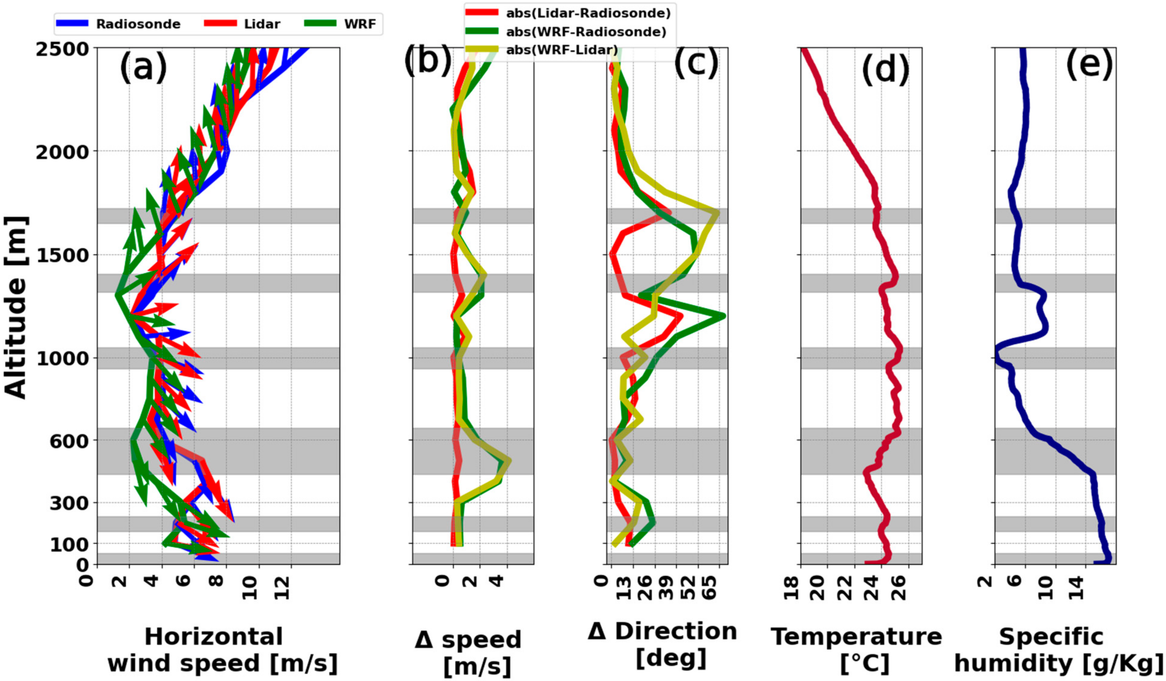
• VAD scans slightly outperformed DBS results for high altitudes (tetheresonde data), which is most probably because of the more detailed data comprising a single scan which includes 24 beams, compared to three beams for DBS. For low altitudes (mast data), DBS scans yield slightly better R² values. This can be attributed to faster changes in lower altitudes which may require faster scans.
• Although spanning a wider area with potential spatial variability, scans with 60° elevation of the LiDAR are advantageous in comparison with 80° scans. This stems from the decrease of vertical wind component presence in the measured signal, combined with the fact the vertical component exhibits enhanced spatial variability, especially in daytime conditions.

It should be noted that the optimal scan type and elevation angle may change for different topography. For example, a DBS should be considered for fast changing flows around obstacles [19], and larger elevations may be unavoidable for flows with strong horizontal heterogeneity.

• Information regarding the existence of MLH and temperature inversions can be obtained through the analysis of backscatter signals and vertical wind standard deviation. For some cases, the existence of temperature inversion layers higher than the MLH can be indirectly detected through gradients in the horizontal wind profile.
• Synergic use of WRF simulations and LiDAR observations is utilized with low SNR LiDAR data replaced by model data.
• In some cases, there is discrepancy between forecasted and observed wind speeds originating from discrepancies in the prediction of inversion layer height.
• Data from standard regional weather prediction models forecasting temperature and mixing ratio profiles may be used for the pre-assessment of SNR as a function of height.

Future work will focus on implementing the combined WRF-LiDAR product exemplified here for a dataset covering a longer period. The dataset will also be used to systematically examine inversion detection through observed horizontal wind gradients and the relation of predicted mixing ratio and LiDAR SNR values.

References

1. Liu, Z.; Barlow, J.F.; Chan, P.W.; Fung, J.C.H.; Li, Y.; Ren, C.; Mak, H.W.L.; Ng, E. A review of progress and applications of pulsed DopplerWind LiDARs. Remote Sens. 2019, 11, 2522. [Google Scholar] [CrossRef]
2. Collier, C.G.; Fay, D.; Karen, E.B.; Holt, A.R.; Middleton, D.R.; Pearson, G.N.; Siemen, S.; Willetts, D.V.; Upton, G.J.G.; Young, R.I. Dual-Doppler lidar measurements for improving dispersion models. Bull. Am. Meteorol. Soc. 2005, 86, 825–838. [Google Scholar] [CrossRef]
3. Pearson, G.; Davies, F.; Collier, C. An analysis of the performance of the UFAM pulsed Doppler lidar for observing the boundary layer. J. Atmos. Ocean. Technol. 2009, 26, 240–250. [Google Scholar] [CrossRef]
4. Wang, Y.; Hocut, C.M.; Hoch, S.W.; Creegan, E.; Fernando, H.J.; Whiteman, C.D.; Felton, M.; Huynh, G. Triple Doppler wind lidar observations during the mountain terrain atmospheric modeling and observations field campaign. J. Appl. Remote Sens. 2016, 10, 26015. [Google Scholar] [CrossRef]
5. Thobois, L.; Cariou, J.P.; Gultepe, I. Review of lidar-based applications for aviation weather. Pure Appl. Geophys. 2019, 176, 1959–1976. [Google Scholar] [CrossRef]
6. Newsom, R.K.; Brewer, W.A.; Wilczak, J.M.; Wolfe, D.E.; Oncley, S.P.; Lundquist, J.K. Validating precision estimates in horizontal wind measurements from a Doppler lidar. Atmos. Meas. Technol. 2017, 10, 1229–1240. [Google Scholar] [CrossRef]
7. Shun, C.M.; Lam, H.K. Remote Sensing of Windshear under Tropical Cyclone Conditions in Hong Kong. In Proceedings of the 35th Session of the Typhoon Committee, Chiang Mai, Thailand, 19–25 November 2002. [Google Scholar]
8. Dehghan, A.; Mariani, Z.; Leroyer, S.; Sills, D.; Bélair, S.; Joe, P. Evaluation of Modeled Lake Breezes Using an Enhanced Observational Network in Southern Ontario: Case Studies. J. Appl. Meteorol. Climatol. 2018, 57, 1511–1534. [Google Scholar] [CrossRef]
9. Curry, M.; Hanesiak, J.; Kehler, S.; Sills, D.M.; Taylor, N.M. Ground-based observations of the thermodynamic and kinematic properties of lake-breeze fronts in southern Manitoba, Canada. Bound. Layer Meteorol. 2017, 163, 143–159. [Google Scholar] [CrossRef]
10. Lemonsu, A.; Bastin, S.; Masson, V.; Drobinski, P. Vertical structure of the urban boundary layer over Marseille under sea-breeze conditions. Bound. Layer Meteorol. 2006, 118, 477–501. [Google Scholar] [CrossRef]
11. Berg, L.K.; Newsom, R.K.; Turner, D.D. Year-Long Vertical Velocity Statistics Derived from Doppler Lidar Data for the Continental Convective Boundary Layer. J. Appl. Meteorol. Climatol. 2017, 56, 2441–2454. [Google Scholar] [CrossRef]
12. Bonin, T.A.; Choukulkar, A.; Brewer, W.A.; Sandberg, S.P.; Weickmann, A.M.; Pichugina, Y.L.; Banta, R.M.; Oncley, S.P.; Wolfe, D.E. Evaluation of turbulence measurement techniques from a single Doppler lidar. Atmos. Meas. Technol. 2017, 10, 3021–3039. [Google Scholar] [CrossRef]
13. Ronen, A.; Tzadok, T.; Rostkier-Edelstein, D.; Agassi, E. Fog measurements with ir whole sky imager and Doppler lidar, combined with in situ instruments. Remote Sens. 2021, 13, 3320. [Google Scholar] [CrossRef]
14. Park, S.; Kim, M.H.; Yeo, H.; Shim, K.; Lee, H.J.; Kim, C.H.; Song, C.K.; Park, M.S.; Shimizu, A.; Nishizawa, T.; et al. Determination of mixing layer height from co-located lidar, ceilometer and wind Doppler lidar measurements: Intercomparison and implications for PM2. 5 simulations. Atmos. Pollut. Res. 2022, 13, 101310. [Google Scholar] [CrossRef]
15. Schween, J.H.; Hirsikko, A.; Löhnert, U.; Crewell, S. Mixing-layer height retrieval with ceilometer and Doppler lidar: From case studies to long-term assessment. Atmos. Meas. Technol. 2014, 7, 3685–3704. [Google Scholar] [CrossRef]
16. Davis, J.C.; Collier, C.G.; Davies, F.; Pearson, G.N.; Burton, R.; Russell, A. Doppler lidar observations of sensible heat flux and intercomparisons with a ground-based energy balance station and WRF model output. Meteorol. Z. 2009, 18, 155–162. [Google Scholar] [CrossRef]
17. Bruno, J.H. Evaluating the Weather Research and Forecasting Model Fidelity for Forecasting Lake Breezes. Ph.D. Thesis, Ohio University, Athens, OH, USA, 2019. [Google Scholar]
18. Päschke, E.; Leinweber, R.; Lehmann, V. An assessment of the performance of a 1.5 μm Doppler lidar for operational vertical wind profiling based on a 1-year trial. Atmos. Meas. Technol. 2015, 142, 203–221. [Google Scholar] [CrossRef]
19. Lane, S.E.; Barlow, J.F.; Wood, C.R. An assessment of a three-beam Doppler lidar wind profiling method for use in urban areas. J. Wind Eng. Ind. Aerodyn. 2013, 119, 53–59. [Google Scholar] [CrossRef]
20. Mariani, Z.; Crawford, R.; Casati, B.; Lemay, F. A multi-year evaluation of Doppler lidar wind-profile observations in the Arctic. Remote Sens. 2020, 12, 323. [Google Scholar] [CrossRef]
21. Santos, P.A.A.; Sakagami, Y.; Haas, R.; Passos, J.C.; Taves, F.F. Lidar measurements validation under coastal condition. Opt. Pura Apl. 2015, 48, 193–198. [Google Scholar] [CrossRef]
22. Araki, R.; Ueda, H.; Ohsawa, T.; Azechi, K.; Komatinovic, N. Offshore wind resource assessment on the west coast of awaji island (comparison between galion doppler lidar and meteorological mast). In Grand Renewable Energy Proceedings Japan Council for Renewable Energy (2018); Japan Council for Renewable Energy: Tokyo, Japan, 2018; p. 175. [Google Scholar]
23. Klaas, T.; Pauscher, L.; Callies, D. LiDAR-mast deviations in complex terrain and their simulation using CFD. Meteorol. Z. 2015, 24, 591–603. [Google Scholar] [CrossRef]
24. Knoop, S.; Bosveld, F.C.; de Haij, M.J.; Apituley, A. A 2-year intercomparison of continuous-wave focusing wind lidar and tall mast wind measurements at Cabauw. Atmos. Meas. Technol. 2021, 14, 2219–2235. [Google Scholar] [CrossRef]
25. Cañadillas, B.; Westerhellweg, A.; Neumann, T. Testing the performance of a ground-based wind LiDAR system. One year intercomparison at the offshore platform FIN01. DEWI-Magazin, 15 February 2011. [Google Scholar]
26. Yair, Y.; Ziv, B. An Introduction to Meteorology, Units 5–7 (Updated and Revised); The Open University of Israel: Ra’anana, Israel, 2014. [Google Scholar]
27. Dayan, U.; Rodnizki, J. The temporal behavior of the atmospheric boundary layer in Israel. J. Appl. Meteorol. 1999, 38, 830–836. [Google Scholar] [CrossRef]
28. Alpert, P.; Rabinovich-Hadar, M. Pre- and post- frontal lin–s—A meso gamma scale analysis over South Israel. J. Atmos. Sci. 2003, 60, 2994–3008. [Google Scholar] [CrossRef]
29. Alpert, P.; Osetinsky, I.; Ziv, B.; Shafir, H. A new season’s definition based on classified daily synoptic systems: An example for the eastern Mediterranean. Int. J. Climatol. 2004, 24, 1013–1021. [Google Scholar] [CrossRef]
30. Tyrlis, E.; Lelieveld, J.; Steil, B. The summer circulation over the eastern Mediterranean and the Middle East: Influence of the South Asian monsoon. Clim. Dyn. 2012, 40, 1103–1123. [Google Scholar] [CrossRef]
31. Hersbach, H.; Bell, B.; Berrisford, P.; Hirahara, S.; Horányi, A.; Muñoz-Sabater, J.; Nicolas, J.; Peubey, C.; Radu, R.; Schepers, D.; et al. The ERA5 global reanalysis Q. J. R. Meteorol. Soc. 2020, 146, 1999–2049. [Google Scholar] [CrossRef]
32. Ganor, E.; Stupp, A.; Alpert, P. A method to determine the effect of mineral dust aerosols on air quality. Atmos. Environ. 2009, 43, 5463–5468. [Google Scholar] [CrossRef]
33. Shellhorn, R.A.; Vaisala, B.O. Advances in Tethered Balloon Sounding Technology. In Proceedings of the 12th Symposium on Meteorological Observations and Instrumentation. 2003. Available online: https://ams.confex.com/ams/pdfpapers/58534.pdf/ (accessed on 4 July 2022).
34. Vaisala Tethersonde TTS111. Available online: https://www.yumpu.com/en/document/read/11364490/vaisala-tethersonde-tts111-hobeco. (accessed on 4 July 2022).
35. Thies Clima Products. Available online: https://www.thiesclima.com/en/Products/Wind-First-Class/ (accessed on 4 July 2022).
36. Skamarock, W.C.; Klemp, J.B.; Dudhia, J.B.; Gill, D.O.; Barker, D.M.; Duda, M.G.; Huang, X.-Y.; Wang, W.; Powers, J.G. A Description of the Advanced Research WRF Model Version 4.3; National Center for Atmospheric Research: Boulder, CO, USA, 2021; p. 145. [Google Scholar]
37. Avisar, D.; Pelta, R.; Chudnovsky, A.; Rostkier-Edelstein, D. High Resolution WRF Simulations for the Tel-Aviv Metropolitan Area Reveal the Urban Fingerprint in the Sea-Breeze Hodograph. J. Geophys. Res. Atmos. 2021, 126, e2020JD033691. [Google Scholar] [CrossRef]
38. Xie, B.; Fung, J.C.H.; Chan, A.; Lau, A. Evaluation of nonlocal and local planetary boundary layer schemes in the WRF model. J. Geophys. Res. 2012, 117, D12103. [Google Scholar] [CrossRef]
39. Kunin, P.; Alpert, P.; Rostkier-Edelstein, D. Study of Sea-breeze/Foehn in the Dead Sea Valley employing High Resolution WRF and Observations. Atmos. Res. 2019, 229, 240–254. [Google Scholar] [CrossRef]
40. Fovell, R.G.; Gallagher, A. Boundary layer and surface verification of the high-resolution rapid refresh, version 3. Weather Forecast. 2020, 35, 2255–2278. [Google Scholar] [CrossRef]
41. Lenchow, D.H.; Wulfmeyer, V.; Sneff, C. Measuring second through fourth-order moments in noisy data. J. Atmos. Ocean. Technol. 2000, 17, 1330–1347. [Google Scholar] [CrossRef]
42. Newsom, R.K.; Krishnamurthy, R. Doppler Lidar (DL) Instrument Handbook No. DOE/SC-ARM/TR-101; DOE Office of Science Atmospheric Radiation Measurement (ARM) User Facility, ARM Data Center: Oak Ridge, YN, USA, 2020.
43. Smalikho, I.N.; Banakh, V.A. Measurements of wind turbulence parameters by a conically scanning coherent Doppler lidar in the atmospheric boundary layer. Atmos. Meas. Technol. 2017, 10, 4191–4208. [Google Scholar] [CrossRef]
44. Stull, R.B. An Introduction to Boundary Layer Meteorology; Springer Science & Business Media: Berlin/Heidelberg, Germany, 1988; Volume 13. [Google Scholar]
45. Zhao, H.; Che, H.; Xia, X.; Wang, Y.; Wang, H.; Wang, P.; Ma, Y.; Yang, H.; Liu, Y.; Wang, Y.; et al. Climatology of mixing layer height in China based on multi-year meteorological data from 2000 to 2013. Atmos. Environ. 2019, 213, 90–103. [Google Scholar] [CrossRef]
46. Brooks, I.M. Finding boundary layer top: Application of a wavelet covariance transform to lidar backscatter profiles. J. Atmos. Ocean. Technol. 2003, 20, 1092–1105. [Google Scholar] [CrossRef]
47. Haeffelin, M.; Angelini, F.; Morille, Y.; Martucci, G.; Frey, S.; Gobbi, G.P.; Lolli, S.; O’dowd, C.D.; Sauvage, L.; Xueref-Remy, I.; et al. Evaluation of mixing-height retrievals from automatic profiling lidars and ceilometers in view of future integrated networks in Europe. Bound. Layer Meteorol. 2012, 143, 49–75. [Google Scholar] [CrossRef]
48. Davis, K.J.; Gamage, N.; Hagelberg, C.R.; Kiemle, C.; Lenschow, D.H.; Sullivan, P.P. An objective method for deriving atmospheric structure from airborne lidar observations. J. Atmos. Ocean. Technol. 2000, 17, 1455–1468. [Google Scholar] [CrossRef]
49. Warner, T.T. Numerical Weather and Climate Prediction; Cambridge University Press: Cambridge, UK, 2011; p. 526. ISBN 978-0-521-51389-0. [Google Scholar]
Figure 1. A map of the campaign layout [© Google maps, Google, Mountain view, CA, USA]. The Meteorological mast height is 115 m above sea level (32°35′11″N, 35°21′36″E). The Study site included the StreamLine-XR and the balloon at (32°34′59″N, 35°21′51″E), 550 m south east to the mast, 88 m above sea level.
Remotesensing 14 04264 g001
Figure 2. Field campaign instrumentation. (a) The streamLine-XR [Halo Photonics, Leigh, England]. (b) Radiosondes [Meteomodem, Ury, France]. (c) EDF meteorological mast at height 100 m. (d) A Tethered balloon [Vaisala, Vantaa, Finland].
Remotesensing 14 04264 g002
Figure 3. Correlation of wind speed and direction (from 30-min averaged data resulting in 74 measurement points, 13–15 September 2021) between LiDAR VAD 60 scans and Tethersondes measurements. (a) Linear scatter plot of horizontal wind speeds. A red dashed line depicts ideal agreement, and the blue solid line is the fitted linear function (b) Average wind direction difference between LiDAR and tethered balloon measurements for VAD 60 scans. The difference is represented by the arc angular extent and the corresponding wind speed by its radial position.
Remotesensing 14 04264 g003
Figure 4. Comparison of DBS 60 scans with mast data. Figure details as in Figure 3.
Remotesensing 14 04264 g004
Figure 5. Wind uniformity for observation of 14 September 2020. Uniformity is expressed by correlation between LOS Doppler speed measurements and sine wave function. (a) for VAD 60. (b) for VAD 80.
Remotesensing 14 04264 g005
Figure 6. LiDAR attenuated backscatter from a “stare” mode scan, 15 September 2020, SNR+1 limited to 1.0095. The grey shaded rectangles represent temperature inversion observed in Radiosonde data. The red solid and dashed vertical lines represent sunrise and sunset, respectively. MLH estimations using σ w threshold and wavelet methods are presented in blue and black solid curves, respectively.
Remotesensing 14 04264 g006
Figure 7. Mean horizontal wind profile in 30-min increments out of LiDAR measurements from VAD 60 scans, 15 September 2020. The arrows indicate the wind direction, while their color shows the wind speed. Each horizontal wind represents a mean of a 30-m layer around the altitude presented. The grey boxes presented are inversion layers with thickness > 50 m extracted from radiosonde temperature data. MLH estimations are repeated from the last figure. The solid and dashed red vertical lines represent sunrise and sunset, respectively.
Remotesensing 14 04264 g007
Figure 8. Log10(SNR) values from a “stare” mode scan, 15 September 2020. Values of SNR+1 lower than 1.0095 are excluded. The black boxes correspond to the time of radiosonde launches. Red vertical solid and dashed lines represent sunrise and sunset, respectively.
Remotesensing 14 04264 g008
Figure 9. Wind profile from WRF model, an average of 30 min interpolated for 100-m gaps. The arrows indicate the wind direction, while their color shows the wind speed. The grey shaded rectangles represent inversion layers with thickness > 50 m extracted from radiosonde temperature data. Shaded red areas correspond to inversions extracted from the forecasted temperature profiles, using the same criteria. The red vertical solid and dashed lines represent sunrise and sunset, respectively.
Remotesensing 14 04264 g009
Figure 10. A combined product of the LiDAR observed wind field (Figure 7) with the WRF modelled wind field (Figure 9). Missing observations due to low SNR are locally replaced by WRF data.
Remotesensing 14 04264 g010
Figure 11. Comparison of LiDAR averaged data from 5:30–6:00, WRF and radiosonde data from 5:53 launch, 15 September 2020. (a) Horizontal wind speed (horizontal axis) and direction (uniform length arrow, with upward direction representing northerly wind) as a function of height (vertical axis), for the radiosonde (blue), LiDAR VAD 60 (red) and WRF (green). (b) Absolute differences of wind speed between LiDAR, radiosonde and WRF, (c) Absolute difference of wind direction between LiDAR, radiosonde and WRF. (d) Radiosonde temperature. (e) Radiosonde specific humidity. The grey layers presented are inversion layers with thickness > 50 m extracted from radiosonde temperature data.
Remotesensing 14 04264 g011
Figure 12. Comparison of LiDAR averaged data from 17:30–18:00, WRF and radiosonde data from 17:57 launch, 15 September 2020. (a) Horizontal wind speed (horizontal axis) and direction (uniform length arrow, with upward direction representing northerly wind) as a function of height (vertical axis), for the radiosonde (blue), LiDAR VAD 60 (red) and WRF (green). (b) Absolute differences of wind speed between LiDAR, radiosonde and WRF, (c) Absolute difference of wind direction between LiDAR, radiosonde and WRF. (d) Radiosonde temperature. (e) Radiosonde specific humidity. The grey layers presented are inversion layers with thickness > 50 m extracted from radiosonde temperature data.
Remotesensing 14 04264 g012
Figure 13. Mixing ratio diurnal profile extracted from WRF runs, 15 September 2020 shaded rectangles mark inversion layers with thickness > 50 m extracted from radiosonde temperature data. Red vertical solid and dashed lines represent sunrise and sunset, respectively.
Remotesensing 14 04264 g013