
Deep-Learning-Based Method for Estimating Permittivity of Ground-Penetrating Radar Targets


1
School of Information and Communication, Guilin University of Electronic Technology, Guilin 541004, China
2
School of Artificial Intelligence, Hezhou University, Hezhou 542899, China
3
Shanxi Transportation Technology R&D Co., Ltd., Taiyuan 030032, China
*
Author to whom correspondence should be addressed.
Remote Sens. 2022, 14(17), 4293; https://doi.org/10.3390/rs14174293
Submission received: 21 July 2022
/
Revised: 18 August 2022
/
Accepted: 29 August 2022
/
Published: 31 August 2022
(This article belongs to the Topic Artificial Intelligence in Sensors)
Abstract
:Correctly estimating the relative permittivity of buried targets is crucial for accurately determining the target type, geometric size, and reconstruction of shallow surface geological structures. In order to effectively identify the dielectric properties of buried targets, on the basis of extracting the feature information of B-SCAN images, we propose an inversion method based on a deep neural network (DNN) to estimate the relative permittivity of targets. We first take the physical mechanism of ground-penetrating radar (GPR), working in the reflection measurement mode as the constrain condition, and then design a convolutional neural network (CNN) to extract the feature hyperbola of the underground target, which is used to calculate the buried depth of the target and the relative permittivity of the background medium. We further build a regression network and train the network model with the labeled sample set to estimate the relative permittivity of the target. Tests were carried out on the GPR simulation dataset and the field dataset of underground rainwater pipelines, respectively. The results show that the inversion method has high accuracy in estimating the relative permittivity of the target.
1. Introduction
GPR has been widely used in shallow subsurface detection using non-destructive remote sensing measurement technology. The GPR transmits electromagnetic pulse signals underground and inverts the received GPR echo data to obtain information such as the shape, size, location, and dielectric parameters of the buried target. The commonly used GPR inversion methods include reverse-time migration (RTM) methods [1], common midpoint (CMP) measurements [2], diffraction tomography (DT) approaches [3], and full wave inversion (FWI) [4]. The migration method converts (or migrates) an unfocused space-time GPR image into a focused one, showing the true location and size of the target, but it cannot get the electromagnetic parameters of the targets [5,6]. The CMP method is usually used to invert the permittivity of the medium, which constructs the propagation equation of electromagnetic waves under different transmission and reception distances by using the B-SCAN data with the change of the transmission and reception distance [7,8]. The DT imaging method is established based on the Fourier Transform and Born approximation, which can be deduced from the linear relationship between the spatial Fourier transform of the object contrast function and the back-scattered field of the targets [9,10]. FWI is a data-fitting technique to estimate the permittivity and conductivity of the medium through the minimization of the distance between the observed data and those predicted by the adopted model [11,12], but this inversion method is very sensitive to the initial model; a poor starting model can easily lead the inversion into a local minimum or cycle skipping.
Fundamentally, estimating the electrical property parameters of the subsurface medium based on the scattered field obtained by GPR entails solving an electromagnetic inverse scattering problem. However, the integral equation describing the distribution of the underground field based on Maxwell’s equations is non-linear and ill-posed. At the same time, the real underground scene is usually more complex, with media that can be lossy and dispersive; this prevents the use of exact inverse procedures in operative cases. For non-linear and ill-posed problems, a large number of research studies have been employed, e.g., Van Den Berg et al. [13] discussed an iterative optimization solution for the non-linear cost function of scattered fields. Babcock et al. [14] implemented a reflection waveform inversion method to calculate the permittivity and conductivity of thin-layer media, which uses a non-linear grid search with a Monte Carlo scheme to initialize starting values to find the global minimum. Feng et al. [15] used a method combining a total-variation model constraint and multi-scale inversion strategy to deal with the ill-posed problem of GPR inversion. A trade-off between accuracy and stability can be established by introducing a regular term and combining linear approximation and regularization strategies, e.g., Feng et al. [16] utilize modified total-variation regularization to constrain the inverted models to improve inversion stability and mitigate ill-posedness. However, the weight parameter of the cost function after adding a regularization term needs to be determined through considerable numerical experimentation, and the linear approximation is usually carried out under the corresponding preconditions. For instance, under the assumption of weak wave field scattering (small disturbance), the Born approximation [17] treats the field component as a perturbation expansion, and the Rytov approximation [18] treats the complex phase of the field component as a perturbation expansion. Therefore, all these factors call for an innovation of the inverse scattered field analysis method.
In recent years, deep-learning methods have been used in the object segmentation [19], detection [20], and identification [21] of optical images with notable success. In the geoscience community, deep-learning methods have also been widely investigated for seismic fault detection [22,23], seismic facies identification [24,25], the detection of target feature hyperbola in GPR B-SCAN images [26,27], and the classification and identification of GPR buried targets et al. [28,29]. In geophysical inversion, deep-learning-based methods have also been used to invert seismic velocity or impedance. For instance, Zhang et al. [30] adopted an adjoint-driven deep-learning FWI method that utilizes the fully convolutional network (FCN) to invert seismic velocity. Ren et al. [31] developed a CNN-based method to estimate seismic velocity. Zhang et al. [32] utilized the ability of DNNs to non-linearly map inputs to expected outputs and perform impedance inversion by a semi-supervised framework. GPR and seismology are both wave-based geophysical techniques; some deep-learning-based methods to inverse GPR scatter field have been introduced in the literature, e.g., Liu et al. [33] developed a trace-to-trace structure of DNN to reconstruct the permittivity map of tunnel linings but did not verify it in the field scenario. Leong et al. [34] proposed a CNN-based method to directly invert the electromagnetic velocity in the subsurface layered structure medium; this method is only for the case where there is no buried target in the layered medium. Ji et al. [35] used a DNN-based method to invert the spatial location, size, and permittivity of objects with different sizes; however, the inversion results in the field scenario have a large deviation. Meanwhile, such methods are data-driven and make use of large data sets to learn the solution to the inverse scattered field. It should be noted that the echo data is obtained under the constraints of the physical mechanism of GPR. To this end, a combined GPR physical model-driven and data-driven approach is proposed to invert the GPR scattering electric field. In this study, we focus on the non-linear mapping transformation based on a regression network to invert the permittivity of buried targets. More specifically, the contributions of this study are as follows:
- (1)
- A method combining the physical mechanism of GPR and using CNN to detect the high-level features of B-SCAN images is proposed to effectively obtain the main parameter information for inversion of the GPR scattering field.
- (2)
- We propose a regression-model-based approach to estimate the permittivity of subsurface targets. Specifically, by analyzing the physical characteristics of the GPR echo data in the reflection measurement mode [36], the target scattering intensity, buried depth, and the permittivity of the background medium are used as input parameters of the regression network, and the estimation result of the target permittivity is output by non-linear mapping transformation.
- (3)
- According to the MAXWELL equations, we discuss the validity of using regression models to estimate target permittivity after generalizing the subsurface half-space from a single-layer medium to a layered structure, which is verified by numerical simulations and field experiments.
The study is organized as follows: we first introduce a combined model-driven and data-driven approach to invert the permittivity of buried targets. Then, we apply the methodology to synthetic data sets and validate the proposed method using field data. Finally, we present our conclusions.
2. Materials and Methods
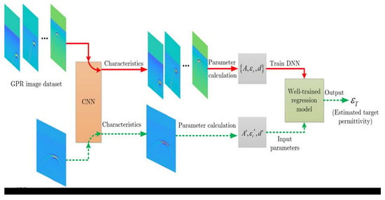
In this section, we focus on the method of building a regression network model to estimate the relative permittivity of the target based on the feature information extracted from the B-SCAN image. It should be noted that in our previous research work [37,38], we analyzed the feature hyperbola detection method of B-SCAN images based on a convolutional neural network (CNN) in detail; the network structure used in this paper is described in Section 2.2.
2.1. GPR Physical Mechanism
In the reflection measurement mode, GPR detects the buried target by transmitting electromagnetic pulse signals into the ground. The distance between the transmit and receive antennas is fixed, and they move together along the azimuth, close to the ground. The echo signal is shown as a function of the measuring point and travel time, and this provides a B-SCAN image, wherein the localized target appears as a diffraction hyperbola that opens downwards. We assume that the incident uniform plane electromagnetic wave can be expressed as
where is the intensity of the incident electromagnetic waves, is the wave number, is the distance between field point and source point, is the angular frequency of the emitted electromagnetic wave. Electromagnetic physical phenomena such as the reflection and refraction of incident waves occur at a dielectric boundary
where and are the reflected wave and refracted wave, respectively. According to Snell’s law [39], reflection coefficient and transmission coefficient are given by
where and are the dielectric constant of medium 1 and medium 2, respectively. It should be noted that the dielectric constant of the medium is a complex number, and its expression is , where represents the real part of the permittivity and is the dielectric loss factor. Consider the attenuation of electromagnetic waves in a lossy medium. Usually, the attenuation is described by the conductivity (S/m) or the electric loss tangent () at a given frequency [40]. The permittivity discussed in this paper refers to the real part of , and the attenuation of the medium is described by the conductivity parameter.
For a lossy medium, it can be deduced from the MAXWELL equations that the amplitude of the incident electromagnetic wave decays exponentially with the distance in the propagation direction [36]. The reflected wave, considering the influence of attenuation factors, can be expressed as
where is the decay factor, and , , and are the relative permittivity, relative permeability, and electrical conductivity of the medium, respectively. In general, the relative permeability of the background medium in the underground half-space is equal to the relative permeability of the air, i.e., , and when the parameter is determined, the soil medium generally satisfies . It can be seen that when the attenuation is constant, the relative permittivity is the main electrical characteristic parameter that affects the scattering intensity. Figure 1 shows the simulated B-SCAN images when different targets are buried in the soil. Figure 1a is an air-filled target, and its relative permittivity is set to 1 and its conductivity is set to 0; Figure 1b is a water-filled target that has a relative permittivity of 81 and a conductivity of 0.03 S/m; the relative permittivity of the background medium soil is 11 and the conductivity is 0.02 mS/m.
As shown in Figure 1, since the phases of the air-filled target and the water-filled target are opposed, the amplitude of the scattered electric field shows an opposite peak. As shown by the characteristic hyperbola of the rectangular area in Figure 1a,b, the amplitude of the air-filled target is negative, and the amplitude of the water-filled medium target is positive. According to Equations (3) and (5), if , the scattered electric field will generate an additional phase; that is, when the electromagnetic wave propagates from a medium with a small permittivity to a medium with a large permittivity, the phase will be reversed. In order to obtain the phase information of , it can be mapped to the complex domain by Hilbert transform and denoted as ; this process can be expressed as
Then, the instantaneous phase calculation formula of the scattered field can be expressed as
where and represent the imaginary part and the real part of the complex number, respectively. By comparing with the phase of the direct wave in the echo signal, the phase change information at the target boundary can be obtained, and the spatial position information of the target feature’s hyperbola in B-SCAN images can be accurately located.
According to the above analysis of the physical mechanism of GPR, it can be seen that the electromagnetic (EM) wave is partly reflected at the interface between two different media and partly transmitted into the next layer. (1) The reflected wave is based on the amplitude strength, proportionally dependent on the relative permittivity for each subsurface layer. The larger the dielectric contrast, the higher the reflection amplitude, and when EM waves pass from a medium with a lower permittivity to a higher one, the reflected waves are out-of-phase with the incident waves. (2) The refracted wave is in phase with the incident wave and propagates into deeper layers, and attenuation increases as the depth increases. Hence, the scattering intensity of the target in the echo signal, the buried depth of the target, and the relative permittivity of the background medium are the main parameters that affect the estimation result of the relative permittivity of the target. Accordingly, in Section 2.4, we take , , and as the input parameters of the regression network to estimate . The acquisition of parameters , , and is related to the characteristic hyperbola of the target, that is, the scattering intensity at the vertex of the characteristic hyperbola corresponds to parameter , and the position of the vertex corresponds to the parameter , and parameter can be calculated by using the geometric relationship of the hyperbola.
Remark 1.
According to the physical mechanism of GPR, we analyze the main factors affecting electromagnetic scattering in the subsurface, such as target scattering intensity, attenuation and phase change of electromagnetic waves, etc., and then determine the relevant parameters for solving the dielectric constant of the target. The prior information obtained based on the GPR physical mechanism is integrated into the DNN model to accurately invert the GPR inverse scattering field.
2.2. CNN-Based Feature Hyperbola Detection Method
The target in the B-SCAN image exhibits a hyperbolic structure with a downward opening and a certain intensity feature. Based on this, we use a CNN-based semantic feature detection network to extract the target feature information in B-SCAN images.
The network structure for extracting semantic features, shown in Figure 2, is mainly composed of two parts: convolution and deconvolution networks. The convolution network is used to extract the high-level semantic information of the input B-SCAN image, and the deconvolutional network up-samples the semantic feature map to obtain a feature map of the same size as the input image. To deal with interfering signals in B-SCAN images, we employ a classifier network to identify target feature hyperbolas. In this paper, the classification network consists of two fully connected layers of size 1 × 1 × 4096 and a softmax activation function.
Remark 2.
Starting from the echo signal, the method of extracting the main parameter information in the GPR data is discussed to invert the permittivity of the target. A CNN-based B-SCAN image feature extraction method was used to obtain the main parameter information of GPR data. Compared with typical neural network models based on anchor boxes and non-anchor boxes, such as the Faster RCNN network and the YOLO series network, the proposed method utilizes the difference in the electrical parameters of target and background media to extract the semantic features of images. Furthermore, according to the B-SCAN image under the constraint of GPR, the target exhibits a hyperbolic structure with a downward opening, and a classification and recognition network is used to identify the target and interference information. This greatly improves the accuracy of extracting feature information from GPR image data in complex scenes.
2.3. Background Dielectric Permittivity Calculation Method
The geometric structure of the target feature hyperbola in the GPR B-SCAN image is shown in Figure 3. The separation distance between the transmitter and receiver of the inner system is fixed, and the GPR moves in the direction with set step size ; ordinate is the two-way travel time, and horizontal coordinate and vertical coordinate , corresponding to the vertex of the hyperbola, indicate the horizontal position and the burial depth of the target, respectively. The corresponding two-way travel time at burial depth is ; denotes the horizontal coordinate of the antenna at the trace; the distance between and the target is denoted as . The following relations can be observed from the geometry in Figure 3.
Let the propagation velocity of the EM wave emitted by GPR in the medium be ; then, , where denotes the two-way travel time from the antenna at position to the buried target. Discretize the axes, i.e., let , , , , and plug them into Equation (9). According to the calculation of , the following equation can be obtained
where and are known quantities. Taking three different coordinate points on the characteristic hyperbola and plugging them into Equation (10) yields the wave speed , and then the relative permittivity of the background medium can be calculated by .
2.4. Regression Network-Based Permittivity Estimation Method
Consider the geometry of the 2D problem depicted in Figure 4. The geometry consists of two half-spaces where the upper half-space is free space, with magnetic permeability and permittivity , respectively. The lower half-space represents the ground, with magnetic permeability and permittivity , respectively, and the target is buried underground. We first use the MAXWELL-based equations to deal with the inverse scattering problem, which is described by the integral relationships.
Assuming that the GPR emits an electromagnetic pulse signal with an angular frequency to the ground, the total scattering field satisfies the Helmholtz equation
where the wave number is given by
When there is no target underground, we define a background wave number corresponding to the underground half-space as
Plugging Equation (13) into Equation (11) yields
where the contrast function is defined as
We introduce Green’s function , which satisfies the following wave equation
The description of the total scattering field can be denoted as
Combining Equations (11) and (16), the equation for calculating the incident field can be obtained as
Since is the sum of and , the result of the subtraction of Equations (17) and (18) is
The process of inverting the target permittivity (which is included in the parameter term ) by Equation (19) can be described as
where is the inverse operation, is the parameter set, including main parameters such as reflection coefficient , attenuation factor , and target burial depth . It can be seen from Equation (20) that under the constraint of the parameter set , an explicit formulation cannot usually be obtained when inverting the GPR inverse scattering field according to . However, it is known from the universal approximation theorem [41] that a fully connected neural network with a large number of neurons in its hidden layer has the ability to represent any function we wish to learn. Based on this, DNN can be used to characterize the inherent non-linear relationship between the observed quantity and the feature information of the input signal :, where is the weight parameter set of DNN. That is, in the expression form, DNN is a non-linear mapping from the observation space to the feature space . For any , can be explicitly expressed as
where is the weight coefficient of the layer of the DNN network, which can be determined by learning, is the depth of the DNN, which can be determined by cross-validation. In order to invert the scattered field equation shown in Equation (19), combined with the physical mechanism of GPR working in the underground half-space and the above data-driven DNN model, we determine the main physical parameters describing the field distribution, such as the target scattered field intensity , the background permittivity , and target burial depth . They are used as the input of the DNN to train the network model and output the estimation results of target permittivity. The designed regression network structure is shown in Figure 5.
The detailed parameters of each layer in the regression network are shown in Table 1.
The following regression network-based algorithm can be implemented to estimate the permittivity :
- (1)
- Make a data set for training the DNN:
- (2)
- The non-linear mapping is expanded into an layer DNN, and the network model is trained on the example set. In general, empirical risk can be used to evaluate the results of model training, that is, to measure the degree of fit between the model and the training set in an average sense, where the empirical risk can be defined as
Gradient descent can be used to solve this optimization problem.
- (3)
- For the observation value of the input DNN, through non-linear mapping transformation, the output value is the parameter inversion result.
Remark 3.
The traditional model-based inverse problem-solving method has the advantage of defining the search space of the solution according to the physical mechanism, but it has the problem of difficulty in accurate modeling and accurate inversion. While learning-based inverse problem-solving methods do not depend on models, their effectiveness inherently depends on network topology and hypothesis space. We propose a combination of physical model-driven and data-driven methods, such as expanding the non-linear mapping process shown in Equation (20) into an L-layer DNN and then optimizing the solution. The main idea is to use the powerful learning ability of neural networks to solve the problems of accuracy and difficult model selection of traditional model methods while using model methods that can solve the difficulties of machine learning in determining network topology and hypothesis space.
3. Results and Analysis
We demonstrate the effectiveness of the regression-network-based method for solving the non-linear mapping problem of the GPR inverse scattering field. Firstly, a numerical simulation experiment is carried out for the situation where the subsurface half-space is a single-layer medium, and the input parameter set of the regression network is determined according to the extracted target feature hyperbola to output the estimated result of target permittivity. Then, according to the MAXWELL equations, the subsurface half-space is extended to the layered media, and the influence on the output prediction results when the input parameters of the regression network have a certain deviation is discussed. Finally, it is verified in field scenes.
3.1. Numerical Simulation Description
The radar parameters are set to the following: the frequency of the GPR transmitting the ricker waveform pulse to the ground is set to 400 MHz, the time window is set to 45 ns, the receiving and transmitting antennas are moved close to the ground, and the distance is set to 0.15 m. In the model structure shown in Figure 4, the lower half-space scene is set up as follows: the width along the azimuth direction is 5 m, and the depth along the range direction is 2 m. The relative permittivity of the background medium is set to 9. The shape of the buried target is set to a rectangle, where the size of the air-filled target is randomly generated between 0.3–0.5 m in width and 0.3–0.4 m in height; the width and height of the water-filled target are randomly generated between 0.25–0.65 m and 0.25–0.45 m, respectively. The targets are randomly distributed in the soil layer, and 1000 images are simulated for each of the air-filled and water-filled targets using the GPRMAX toolbox [42]; a total of 2000 B-SCAN images are obtained.
According to the MAXWELL equations, we can generalize the model with a single-layer medium in the lower half-space shown in Figure 4 to the case of a layered medium. As shown in Figure 6, the lower half-space consists of a concrete layer and a soil layer, and the target is located in the soil layer.
In the layered structure shown in Figure 6, the specific parameters of the underground scene are set as follows:
- (1)
- The width along the azimuth direction is 5 m, the depth along the range direction is 2 m, and the average thickness of the concrete layer is 0.25 m.
- (2)
- There are 4–6 concave and convex blocks with a maximum width and height of 0.3 m and 0.05 m, respectively, which are randomly generated at the lower boundary of the concrete layer to simulate the rough interface between concrete and soil.
- (3)
- The permittivity of soil along the range direction is generated in a random way; considering the influence of water content in soil at different depths, the range is set to 9–25.
- (4)
- The number of targets is set to 1 or 2, and the shape is set to a rectangle (the size of the air-filled target is randomly generated between 0.3–0.5 m in width and 0.3–0.4 m in height; the width and height of the water-filled target are randomly generated between 0.25–0.65 m and 0.25–0.45 m, respectively). A single target is randomly distributed in the soil layer, and two targets are randomly distributed in the left and right half of the soil layer, respectively.
Under the above scenario settings, a total of 4000 images are obtained, in which the targets are air-filled and water-filled media, the number is 1 and 2, respectively, and 1000 images are simulated for each setting.
3.2. Simulation Results and Analysis
3.2.1. Single-Layer Background Medium Scene
In the single-layer background medium scene, the B-SCAN images (with the direct wave signal removed) of the air-filled target and the water-filled target are shown in Figure 7a,c. It should be noted that all B-SCAN images in the following figure indicate that the direct wave interference signal has been removed. A CNN feature extraction network model, with the structure shown in Figure 2, is used to extract the feature hyperbolas of the target, and the result of fitting the hyperbola by the least squares (LS) method is shown in the red curves in Figure 7b,d.
To verify the validity of the result of the permittivity of the background medium calculated using the geometric relationship shown in Figure 3, we selected 100 images from a sample of 2000 B-SCAN images for testing, including 50 images of each of the air-filled and water-filled targets. The calculation results of , corresponding to each test image, are shown in Figure 8.
The calculated value of ranges from 8.58 to 9.41, and the reference value of is set to 9. The maximum deviation of the results is 0.42, and the average deviation is 0.16. It can be seen that using the geometric relationship to estimate can obtain higher accuracy. Further, the results of the target relative permittivity estimated by the regression model are analyzed. For the 2000 B-SCAN images simulated in the scenario shown in Figure 4, the corresponding parameters , , and are calculated according to the target feature hyperbola extracted from each image, forming a data set with a sample size of 2000. In total, 100 sets of data were selected as the verification set (50 sets of data for air-filled medium targets and 50 sets of water-filled medium targets each), 100 sets of data were selected as test sets (50 sets of data for air-filled medium targets and 50 sets of water-filled medium targets each), and the remaining 1800 sets of data were used as training sets. The validation set is mainly used for tuning the hyperparameters of the DNN model. In our training, the epoch was set to 100 and the batch size was set to 100; the mean squared error function was used as the loss function (the mean of the squared errors between our target and predicted values), and the optimizer adopted ‘Adam’. After 20 epochs, the model training tends to be stable; the change curves of the loss functions of the training set and the validation set are shown in Figure 9.
For 100 sets of test data, the estimation results using the regression model are shown in Figure 10.
It can be seen that the DNN network has high accuracy in estimating the relative permittivity results of the air-filled and water-filled targets, with an average accuracy of 99.27% and 99.13%, respectively. This is the estimation result of under the condition of accurately labeling the parameters , , and . When analyzing the background medium of the layered structure in Section 3.2.2, we will further discuss the influence of the parameters and on the estimation results when there is a certain deviation.
3.2.2. Layered Background Medium Scene
In this section, we extend the underground half-space from a single-layer medium to a layered medium, where the calculation results of the permittivity of the background medium are usually averaged and the data processing procedure for estimating the target permittivity is similar. First, the results of extracting the feature hyperbolas of the target in the B-SCAN image using CNN are shown in Figure 11.
The results shown in Figure 11a–d indicate that the GPR B-SCAN image contains one cavity target, one water-filled medium target, two cavity targets, and two water-filled medium targets, respectively. The LS method is used to fit the target feature hyperbola in the GPR B-SCAN image, and the result is shown in the red curve in Figure 11. Then, use the geometric relationship to calculate the relative permittivity of the background medium, and 100 images are selected from the 4000 simulated images for testing. The calculation result of is shown in Figure 12.
In the model structure shown in Figure 6, since the simulation scene is set as a layered structure, for each B-SCAN image, the result of calculating represents the mean value of the relative permittivity of the background medium. In order to quantitatively analyze the validity of calculating the mean value of using Equation (10), on the one hand, according to the target burial depth set in the simulation process and the two-way travel time corresponding to the vertex of the target feature hyperbola in the B-SCAN image, the average wave speed can be calculated according to , and the average value of the relative permittivity of the background medium can be obtained according to ; this is used as a reference. The calculation results are shown in the blue curve in Figure 12. On the other hand, selecting three different coordinate points on the fitted hyperbola and plugging them into Equation (10) yields the average wave velocity , and the approximate result of the background relative permittivity can be obtained according to . The result is shown as the black curve in Figure 12. Comparing the values of and , we can see that deviates from in the range of 0.01–0.95, and the average difference between and is 0.44.
Compared with the single-layer uniform background medium model shown in Figure 4, the electromagnetic scattering under the layered structure is more complicated, and the averaging method will also introduce certain errors. These factors produced greater deviations in the final results for calculating the background dielectric permittivity, but the calculation results on the test samples are generally satisfactory.
To train the regression network model and predict the permittivity of the target, for the 4000 B-SCAN images simulated in the scenario shown in Figure 6, the corresponding parameters , , and are calculated according to the target feature hyperbola extracted from each image, forming a data set with a sample size of 4000. In total, 200 sets of data were selected as the validation set (100 sets of data for air-filled medium targets and 100 sets of water-filled medium targets each), 200 sets of data were selected as the test set (100 sets of data for air-filled medium targets and 100 sets of water-filled medium targets each), and the remaining 3600 sets of data were used as the training set. In our training, the epoch was set to 100, the batch_size was set to 200, the mean squared error function was used as the loss function, and the optimizer adopted ‘Adam’. After 30 epochs, the model training tends to be stable; the change curves of the loss functions of the training set and the validation set are shown in Figure 13.
The above trained regression network is used to predict the permittivity of the targets; the prediction results on 200 test images are shown in Figure 14.
When the background medium is a layered structure, the average accuracy of the estimation results for the permittivity of the cavity and water-filled targets is 98.85% and 98.30%, respectively. Comparing the calculation results shown in Figure 10 and Figure 14, it is clear that the accuracy of the output results of the regression network is also higher after the subsurface half-space is extended from a single-layer medium to a layered medium. It can be seen that under the condition of effectively obtaining the input parameters , and , the non-linear mapping transformation shown in Equation (20) can be well solved using the DNN.
Due to the complexity of the geological environment, in order to discuss the influence of the deviation of parameters and on the prediction results, we calculated the prediction errors under different deviation degrees. Specifically, the deviation of parameter is within the range of 25%, 100 random deviations are generated at 5% intervals each time, and the deviation corresponding to is set according to the computational relationship equation between and . For the test sample set containing 200 groups of data, the mean value of the prediction error on 100 random deviations was calculated separately for each group of test data, and the statistical results are shown in Figure 15.
As the degree of deviation of parameters and increases, there is an overall decreasing trend in the accuracy of the estimation results for parameter . When the range of and deviations from the reference value increases from 5% to 25%, the average accuracy of the target permittivity estimation results for air-filled and water-filled media will also decrease from 97.37% and 97.30% to 85.04% and 84.77%, respectively. Among them, the maximum estimated deviation values are 0.23 (ground truth of ) and 18.89 (ground truth of ). From the results of the average precision and maximum deviation of the above statistics, although there is a certain error in the estimated value of , according to the typical values of the electrical characteristic parameters of common underground targets, air and water are not misidentified as other types of media at this time. In the experiment, we further increase the deviation values of parameters and . For example, when the deviation range is increased to 35%, the maximum deviation values of the estimated permittivity of the air-filled and water-filled targets are 1.03 and 33.56, respectively, which is prone to misjudgment. It can be seen that in the presence of small deviations in the input parameters of the DNN, the effective judgment of the target medium type can be realized according to the output results of the network, and the designed regression model has a certain robustness.
3.3. Field Results and Analysis
In order to verify the effect of the proposed regression network model on the field data set, the LAUREL radar shown in Figure 16a was used to detect the underground rainwater pipes buried in an industrial park in Shanxi, China. Figure 16b shows the rainwater pipe under the manhole cover. The main working parameters of the impulse radar were set as follows: the working mode was “wheel”; the working frequency was 400 MHz; the number of sampling points was set to 512; the trace sampling interval was 0.04 m; the time window was 100 ns. In the process of data collection, referring to the construction drawings of buried underground rainwater pipelines, the length of the detected pipelines along the pipeline laying direction was 1.2 km in total. The B-SCAN image corresponding to a detection area in the echo data is shown in Figure 16c.
According to the measured data shown in Figure 16c, in the process of making the training set, one trace of the echo data was taken every 1 m in length, and the obtained measured data set contained a total of 1100 groups of data, of which 1000 groups were used for training and 100 groups were used for testing. Taking the pipeline burial depth () designed during construction as a reference, the average wave velocity can be calculated according to the two-way travel time corresponding to the upper boundary of the pipeline in the B-SCAN image. The relative permittivity of background media can be further obtained by using the relationship between the wave velocity of electromagnetic waves in the medium and free space. The DNN model is trained according to the prepared measured parameter set , and the estimation results of the relative permittivity of the target on the test set are shown in Figure 17.
In order to simplify the analysis process, it is assumed that the filling in the pipeline is an air medium; that is, the target to be detected is equivalent to an air-filled medium. From the statistical results on the test set, the average accuracy rate reached 95.52%, and the target relative permittivity estimation results ranged from 0.93 to 1.05. Further, we check the validity of the proposed method with respect to standard inversion processes.
In traditional parameter inversion methods, FWI is the state-of-art solution to quantitatively estimate the parameters of a medium. To demonstrate the superiority of the DNN-based parameter inversion method, a comparative analysis is carried out with the FWI-based parameter inversion algorithm [33]. The statistical test results under the field scenario are shown in Table 2.
It can be seen that the DNN-based method has better performance than the FWI-based method. In terms of the computational cost, the FWI-based algorithm takes approximately 2820 s to complete the inversion for a B-SCAN image with a size of 1428 × 563. In contrast, a well-trained DNN is capable of inverting a set of test data within approximately 0.023 s. The time-consumption of the above-mentioned DNN-based method only refers to the time used to invert the permittivity according to the input parameters , , and and does not include the time used to calculate the parameters in the parameter set and the time consumed to train the regression model. Although making the parameter set and using it to train the DNN is a computationally intensive process, it takes place only once. The well-trained regression model can be used with near real-time speed for processing a set of GPR image data. In terms of the complexity of the implementation, the proposed method starts from the GPR image data and uses the CNN with the cascade structure shown in Figure 2 to automatically extract the feature information of the target and directly calculate the parameters , , and from the fitted curve and the geometric relationship shown in Figure 3 for the inversion of target permittivity. This method can be extended to medium parameter estimation for other subsurface targets. In contrast, FWI is sensitive to the initial model, and it also encounters two bottlenecks: non-linearity and ill-posedness. In practical applications, it usually needs to be improved according to the actual scenario.
The reason why our method is better than FWI is that, on the one hand, for the FWI method, it can be seen from Equations (15) and (19) that the wave number is a key factor affecting the inversion results. When the frequency of the electromagnetic pulse emitted by GPR is constant, the relative permittivity of the background medium is the main factor affecting the estimation result of the target permittivity, and it is very difficult to accurately estimate the inhomogeneous and anisotropic background medium. On the other hand, due to the non-linear and ill-posed problems of the FWI method, the corresponding approximations are generally required (such as Born approximation or Rytov approximation, etc.), and this process also generates certain errors. In addition, the DNN method learns the non-linear mapping relationship between the input parameter set of the regression network and the output estimate of the target relative permittivity through a large number of samples, and the numerical simulation results in Section 3.2.2 show that the DNN method has certain robustness. This conclusion is further validated by the test results on the above field datasets.
It should be noted that considering the detection process of underground pipelines in actual projects, when collecting data, we detect along the laying direction of the pipeline. At this time, affected by factors such as azimuth resolution, the target in the echo data does not show typical hyperbolic structure features; the corresponding B-SCAN image is shown in Figure 16c. The relative permittivity of the background medium cannot be calculated according to the hyperbolic geometric constraint shown in Figure 3. In this regard, in the process of making the data set, we sampled the echo data shown in Figure 16c in segments; this process does not affect the validity of the regression network for verifying the parameter estimation results.
4. Discussion
This study investigates the problem of estimating dielectric constants of subsurface targets using deep learning. We discuss the data processing procedure of inverting target permittivity using the extracted feature hyperbola from the GPR echo data, in which the subsurface half-space is extended from a single-layer medium to a layered medium. Through GPR numerical simulation, the accuracy of the medium parameter estimation results obtained by the proposed method is very high. For the field case study, the predicted results matched the ground truth data very well. Our method shows that deep-learning-based inversion can not only perform GPR scatter field inversion accurately but also quickly and efficiently.
Our approach focuses on building a framework for solving GPR inverse scattered fields that combines model solving and example learning. The scattered field equation shown in Equation (19) is derived from the MAXWELL equations, and the corresponding inverse model (shown in Equation (21)) is given. This non-linear scattering field equation is usually solved iteratively. Here, we trained the DNN by generating a large number of 2D profile data sets and learned the non-linear mapping relationship from the observation space to the feature space to output the parameter estimation results. Our method provides a new way to solve the GPR inverse scattering field problem.
We acknowledge that there are certain differences between the constructed geoelectric model and the real underground scene and that the geological structure we consider is idealistic and simplified. In order to verify the effectiveness of the proposed algorithm, in the numerical simulation experiment, we discussed the error of the output result when the input parameters of the regression network model have different deviations and we also conducted field experiments. The statistical results show that the proposed method has a certain anti-interference ability. However, in the practical application of GPR parameter inversion, the background medium is usually inhomogeneous and anisotropic, and the geological environment in natural scenes is complex and variable. In particular, when the water content of the background medium in the lower half-space is different, the corresponding relative permittivity will change greatly, which will lead to a larger error in the parameter prediction results. In this regard, it is necessary to collect more data in different geological environments to augment the training sample set to improve the generalization performance of the network. We strongly believe that our method can achieve high accuracy results when there are no significant anomalies in the input parameters of the regression model.
The proposed method for inversion of the permittivity of subsurface targets using example learning under the constraints of the GPR physical mechanism can be extended to other inverse problems. For future research, we will further investigate the multi-parameter (e.g., permittivity and conductivity) inversion problem of dielectric material to better reconstruct the underground scene.
5. Conclusions
In this study, we designed a regression model based on DNN to estimate the permittivity of buried targets. Since the inverse scattering field is non-linear and ill-posed, by using the labeled sample set to train the regression model, the regression network can learn the intrinsic non-linear mapping relationship between output and input parameters. The main input parameters of the regression network, such as the permittivity of the background medium, the buried depth of the target, and the scattering intensity, are determined by combining the GPR physical mechanism and the scattering field equation, and the complete data processing process, from the GPR echo signal to the relative permittivity estimation results of the subsurface target, is analyzed.
Overall, the combined physical-model-driven and data-driven method proposed in this paper can accurately estimate the relative permittivity of subsurface targets. Numerical simulation results show the robustness of the designed regression network, and, in the actual measurement scenario, the accuracy of the prediction results of the method in this paper is also high. The simulation and field experimental results show the feasibility of the method in this paper for the inversion of dielectric parameters in complex scenarios.
Author Contributions
Conceptualization, H.W. and S.O.; methodology, H.W. and S.O.; software, H.W.; validation, H.W. and S.O.; formal analysis, S.O., Q.L. and K.L.; investigation, H.W. and S.O.; resources, S.O.; data curation, H.W. and L.Z.; supervision, S.O., Q.L. and K.L. All authors have read and agreed to the published version of the manuscript.
Funding
This work is supported by the National Natural Science Foundation of China (No. 61871425 and No. 61861011), the Guangxi special fund project for innovation-driven development (No. GuikeAA21077008), Shanxi Transportation Technology R&D Co. Ltd., and the Innovation Development Plan Unveiling Project (21-JKCF-55).
Institutional Review Board Statement
Not applicable.
Informed Consent Statement
Not applicable.
Data Availability Statement
The data presented in this study are available upon request from the author H.W.; e-mail: [email protected].
Conflicts of Interest
The authors declare no conflict of interest.
References
- Shen, R.; Zhao, Y.; Hu, S.; Li, B.; Bi, W. Reverse-time migration imaging of ground-penetrating radar in NDT of reinforced concrete structures. Remote Sens. 2021, 13, 2020. [Google Scholar] [CrossRef]
- Liu, S.; Lu, Q.; Li, H.; Wang, Y. Estimation of moisture content in railway subgrade by ground penetrating radar. Remote Sens. 2020, 12, 2912. [Google Scholar] [CrossRef]
- Mangel, A.R.; Moysey, S.; Bradford, J. Reflection tomography of time-lapse GPR data for studying dynamic unsaturated flow phenomena. Hydrol. Earth Syst. Sci. 2020, 24, 159–167. [Google Scholar] [CrossRef]
- Liu, T.; Klotzsche, A.; Pondkule, M.; Vereecken, H.; Su, Y.; van der Kruk, J. Radius estimation of subsurface cylindrical objects from ground-penetrating-radar data using full-waveform inversion. Geophysics 2018, 83, H43–H54. [Google Scholar] [CrossRef]
- Zhong, S.; Wang, Y.; Zheng, Y.; Chang, X. Reverse time migration of ground-penetrating radar with full wavefield decomposition based on the Hilbert transform. Geophys. Prospect. 2020, 68, 1097–1112. [Google Scholar] [CrossRef]
- Xiao, J.; Tang, X.; Liang, B.; Han, F.; Liu, H.; Liu, Q.H. Subsurface reconstruction from GPR data by 1-D DBIM and RTM in frequency domain. IEEE Geosci. Remote Sens. Lett. 2020, 17, 582–586. [Google Scholar] [CrossRef]
- Wang, H.H.; Liu, H.; Cui, J.; Hu, X.Y.; Sato, M. Velocity analysis of CMP gathers acquired by an array GPR system ‘Yakumo’: Results from field application to tsunami deposits. Explor. Geophys. 2018, 49, 669–674. [Google Scholar] [CrossRef]
- Vânia, M.; Fontul, S.; Solla, M.; Antunes, M.D.L. Evaluation of the feasibility of common mid-point approach for air–coupled GPR applied to road pavement assessment. Measurement 2018, 128, 295–305. [Google Scholar] [CrossRef]
- Monte, L.; Erricolo, D.; Soldovieri, F.; Wicks, M.C. Radio frequency tomography for tunnel detection. IEEE Trans. Geosci. Remote Sens. 2010, 48, 1128–1137. [Google Scholar] [CrossRef]
- Qu, L.; Yin, Y.; Sun, Y.; Zhang, L. Diffraction tomographic ground-penetrating radar multibistatic imaging algorithm with compressive frequency measurements. IEEE Geosci. Remote Sens. Lett. 2015, 12, 2011–2015. [Google Scholar] [CrossRef]
- Zhou, Z.; Klotzsche, A.; Schmack, J.; Vereecken, H.; Van Der Kruk, J. Improvement of ground-penetrating radar full-waveform inversion images using cone penetration test data. Geophysics 2021, 86, H13–H25. [Google Scholar] [CrossRef]
- Feng, D.; Wang, X.; Zhang, B. A frequency-domain quasi-newton-based biparameter synchronous imaging scheme for ground-penetrating radar with applications in full waveform inversion. IEEE Trans. Geosci. Remote Sens. 2021, 59, 1949–1966. [Google Scholar] [CrossRef]
- Van den Berg, P.M.; Abubakar, A. Contrast source inversion method: State of art. Prog. Electromagn. 2001, 34, 189–218. [Google Scholar] [CrossRef]
- Babcock, E.; Bradford, J.H. Reflection waveform inversion of ground-penetrating radar data for characterizing thin and ultrathin layers of nonaqueous phase liquid contaminants in stratified media. Geophysics 2015, 80, H1–H11. [Google Scholar] [CrossRef]
- Feng, D.S.; Wang, X.; Zhang, B. Improving reconstruction of tunnel lining defects from ground-penetrating radar profiles by multi-scale inversion and bi-parametric full-waveform inversion. Adv. Eng. Inform. 2019, 41, 100931. [Google Scholar] [CrossRef]
- Feng, D.S.; Ding, S.Y.; Wang, X. Wavefield reconstruction inversion of GPR data for permittivity and conductivity models in the frequency domain based on modified total variation regularization. IEEE Trans. Geosci. Remote Sens. 2022, 60, 1–14. [Google Scholar] [CrossRef]
- Persico, R.; Bernini, R.; Soldovieri, F. The role of the measurement configuration in inverse scattering from buried objects under the born approximation. IEEE Trans. Antennas Propag. 2005, 53, 1875–1887. [Google Scholar] [CrossRef]
- Oliveri, G.; Poli, L.; Rocca, P.; Massa, A. Bayesian compressive optical imaging within the Rytov approximation. Opt. Lett. 2012, 37, 1760–1762. [Google Scholar] [CrossRef]
- Yang, Y.; Lai, B.; Soatto, S. DyStaB: Unsupervised object segmentation via dynamic-static bootstrapping. In Proceedings of the 2021 IEEE/CVF Conference on Computer Vision and Pattern Recognition, Nashville, TN, USA, 19–25 June 2021. [Google Scholar] [CrossRef]
- Fan, Q.; Zhuo, W.; Tang, C.K.; Tai, Y.W. Few-shot object detection with attention-RPN and multi-relation detector. In Proceedings of the 2020 IEEE/CVF Conference on Computer Vision and Pattern Recognition, Seattle, WA, USA, 13–19 June 2020. [Google Scholar] [CrossRef]
- Li, H.; Wu, G.; Zheng, W.S. Combined depth space based architecture search for person re-identification. In Proceedings of the 2021 IEEE/CVF Conference on Computer Vision and Pattern Recognition, Nashville, TN, USA, 19–25 June 2021. [Google Scholar] [CrossRef]
- Zhou, R.S.; Yao, X.M.; Wang, Y.J.; Hu, G.M.; Yu, F.C. Seismic fault detection with progressive transfer learning. Acta Geophys. 2021, 69, 2187–2203. [Google Scholar] [CrossRef]
- Gao, K.; Huang, L.; Zheng, Y. Fault detection on seismic structural images using a nested residual U-net. IEEE Trans. Geosci. Remote Sens. 2022, 60, 1–15. [Google Scholar] [CrossRef]
- Wrona, T.; Pan, I.; Gawthorpe, R.L.; Fossen, H. Seismic facies analysis using machine learning. Geophysics 2018, 83, O83–O95. [Google Scholar] [CrossRef]
- Wang, Z.; Li, F.; Taha, T.R.; Arabnia, H.R. Improved automating seismic facies analysis using deep dilated attention autoencoders. In Proceedings of the 2019 IEEE/CVF Conference on Computer Vision and Pattern Recognition Workshops, Long Beach, CA, USA, 15–20 June 2019. [Google Scholar] [CrossRef]
- Pham, M.T.; Lefèvre, S. Buried object detection from B-scan ground penetrating radar data using Faster-RCNN. In Proceedings of the IEEE International Geoscience and Remote Sensing Symposium, Valencia, Spain, 22–27 July 2018. [Google Scholar] [CrossRef]
- Lei, W.T.; Hou, F.F.; Xi, J.C.; Tan, Q.Y. Automatic hyperbola detection and fitting in GPR B-SCAN image. Autom. Constr. 2019, 106, 102839. [Google Scholar] [CrossRef]
- Yang, J.; Duan, Y.L. Wavelet scattering network-based machine learning for ground penetrating radar imaging: Application in pipeline identification. Remote Sens. 2020, 12, 3655. [Google Scholar] [CrossRef]
- Tong, Z.; Gao, J.; Zhang, H. Recognition location measurement and 3D reconstruction of concealed cracks using convolutional neural networks. Constr. Build. Mater. 2017, 146, 775–787. [Google Scholar] [CrossRef]
- Zhang, W.; Gao, J.; Gao, Z.; Chen, H. Adjoint-driven deep-learning seismic full-waveform inversion. IEEE Trans. Geosci. Remote Sens. 2021, 59, 8913–8932. [Google Scholar] [CrossRef]
- Ren, Y.X.; Liu, B. Seismic data inversion with acquisition adaptive convolutional neural network for geologic forward prospecting in tunnels. Geophysics 2021, 86, 659–670. [Google Scholar] [CrossRef]
- Zhang, H.; Yang, P.; Liu, Y.; Luo, Y.; Xu, J. Deep learning-based low-frequency extrapolation and impedance inversion of seismic data. IEEE Geosci. Remote Sens. Lett. 2022, 19, 1–5. [Google Scholar] [CrossRef]
- Liu, B.; Ren, Y.X.; Liu, H.C.L. GPRInvNet: Deep learning-based ground penetrating radar data inversion for tunnel lining. IEEE Trans. Geosci. Remote Sens. 2021, 59, 8305–8325. [Google Scholar] [CrossRef]
- Leong, Z.X.; Zhu, T. Direct velocity inversion of ground penetrating radar data using GPRNet. J. Geophys. Res. Solid Earth 2021, 126, 21047. [Google Scholar] [CrossRef]
- Ji, Y.T.; Zhang, F.K.; Wang, J.; Wang, Z.F.; Jiang, P.; Liu, H.C.; Sui, Q.M. Deep neural network-based permittivity inversions for ground penetrating radar data. IEEE Sens. J. 2021, 21, 8172–8818. [Google Scholar] [CrossRef]
- Wang, H.; Ouyang, S.; Liao, K.F.; Jing, N.L. GPR B-SCAN image hyperbola detection method based on deep learning. Actc Electron. Sin. 2021, 49, 953–963. [Google Scholar] [CrossRef]
- Wang, H.; Ouyang, S.; Liu, Q.H.; Liao, K.F.; Zhou, L.J. Buried target detection method for ground penetrating radar based on deep learning. J. Appl. Remote Sens. 2022, 16, 018503. [Google Scholar] [CrossRef]
- Wang, H.; Ouyang, S.; Liu, Q.H.; Liao, K.F.; Zhou, L.J. Structure feature detection method for ground penetrating radar two-dimensional profile image based on deep learning. J. Electron. Inf. Technol. 2022, 44, 1284–1294. [Google Scholar] [CrossRef]
- Mendonca, J.T.; Shukla, P.K. Time Refraction and Time Reflection: Two Basic Concepts. Phys. Scr. 2002, 44, 160–163. [Google Scholar] [CrossRef]
- Balanis, C.A. Advanced Engineering Electromagnetics; Wiley: New York, NY, USA, 1989; pp. 73–84. [Google Scholar]
- Hornik, K.; Stinchcombe, M.; White, H. Universal approximation of an unknown mapping and its derivatives using multilayer feedforward networks. Neural Netw. 1990, 3, 551–560. [Google Scholar] [CrossRef]
- Warren, C.; Giannopoulos, A.; Giannakis, I. GPRMAX: Open source software to simulate electromagnetic wave propagation for ground penetrating radar. Comput. Phys. Commun. 2016, 209, 163–170. [Google Scholar] [CrossRef] [Green Version]
Figure 1.
GPR B-SCAN images.
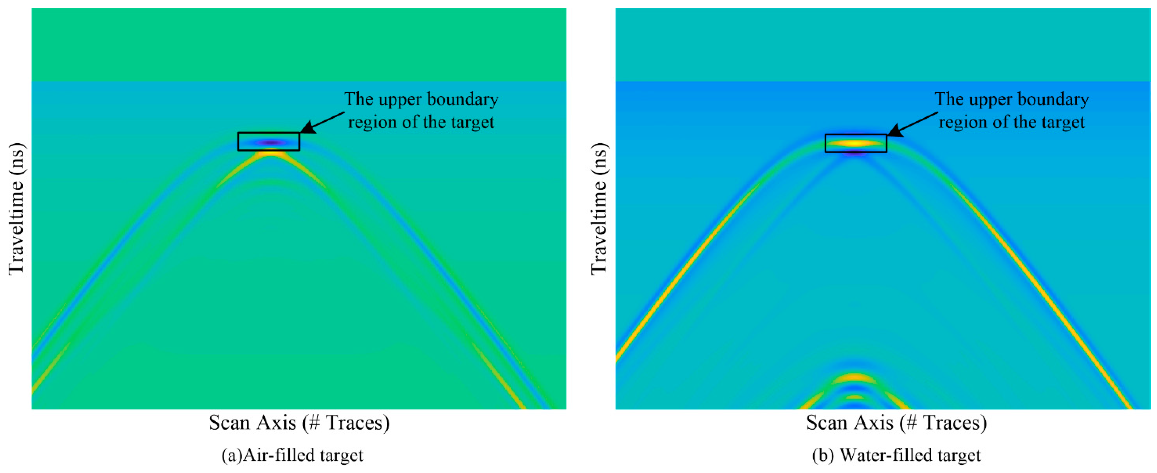
Figure 2.
Structure diagram of the B-SCAN image feature curve extraction network.
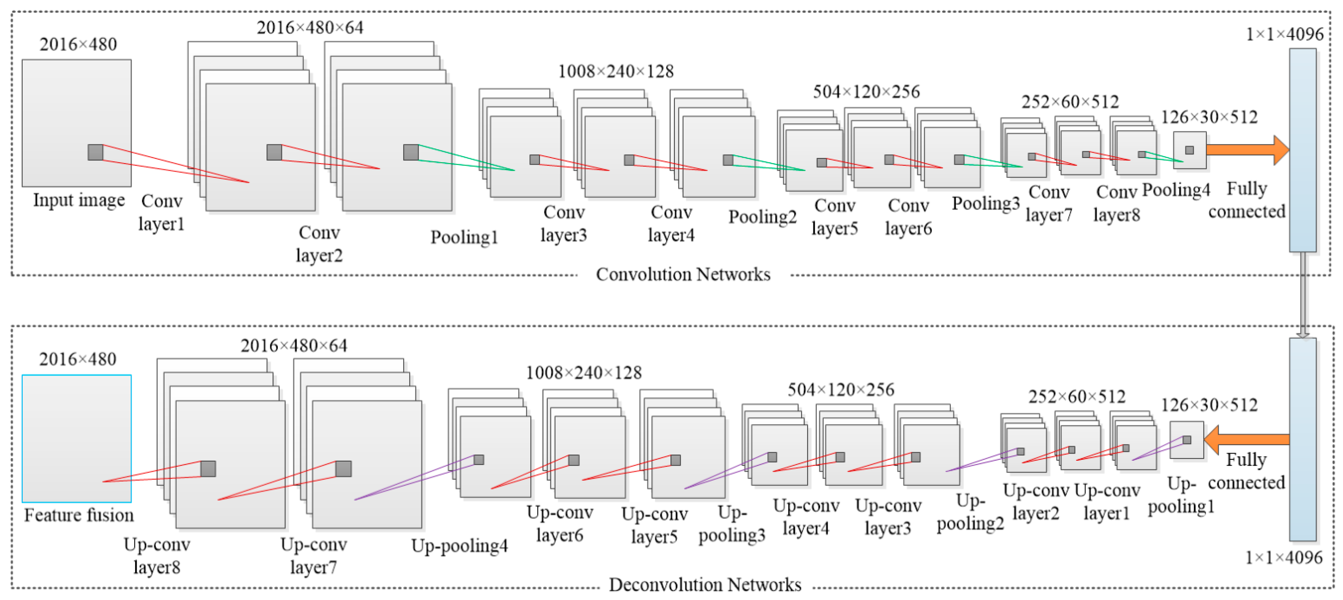
Figure 3.
Geometric relationship of the buried target.
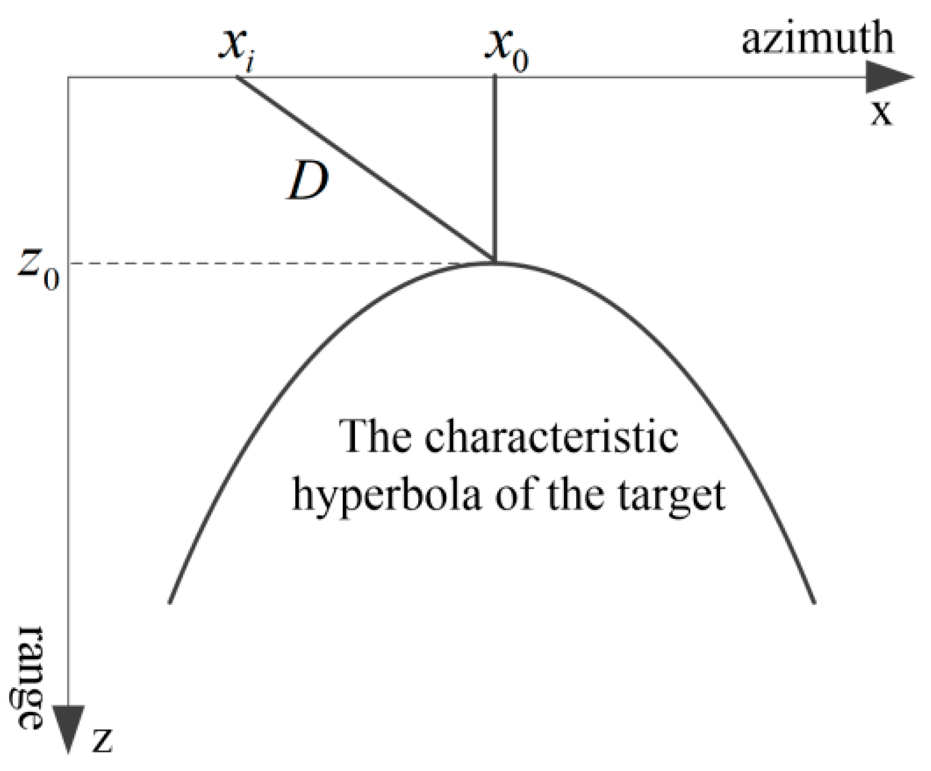
Figure 4.
The geometry for a 2D problem.
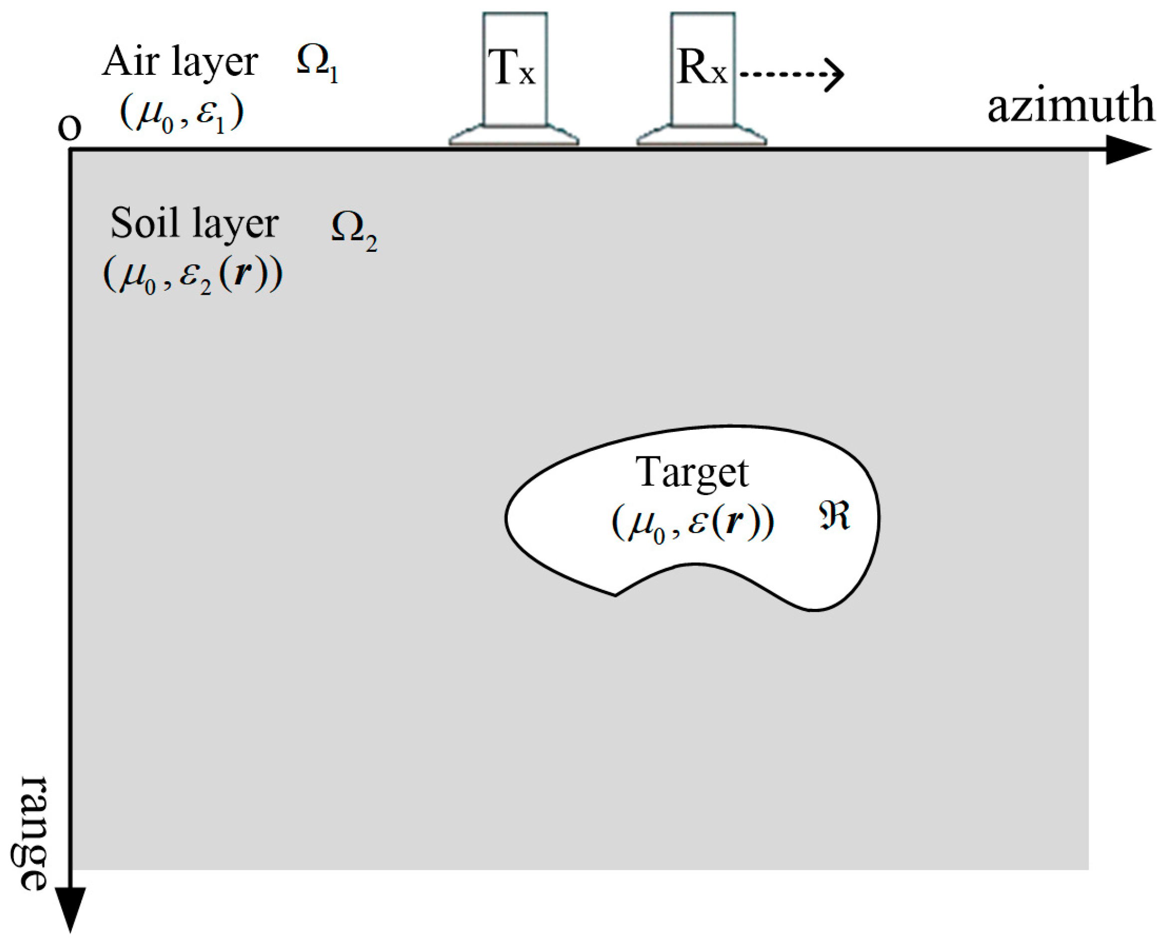
Figure 5.
The structure of the proposed DNN.
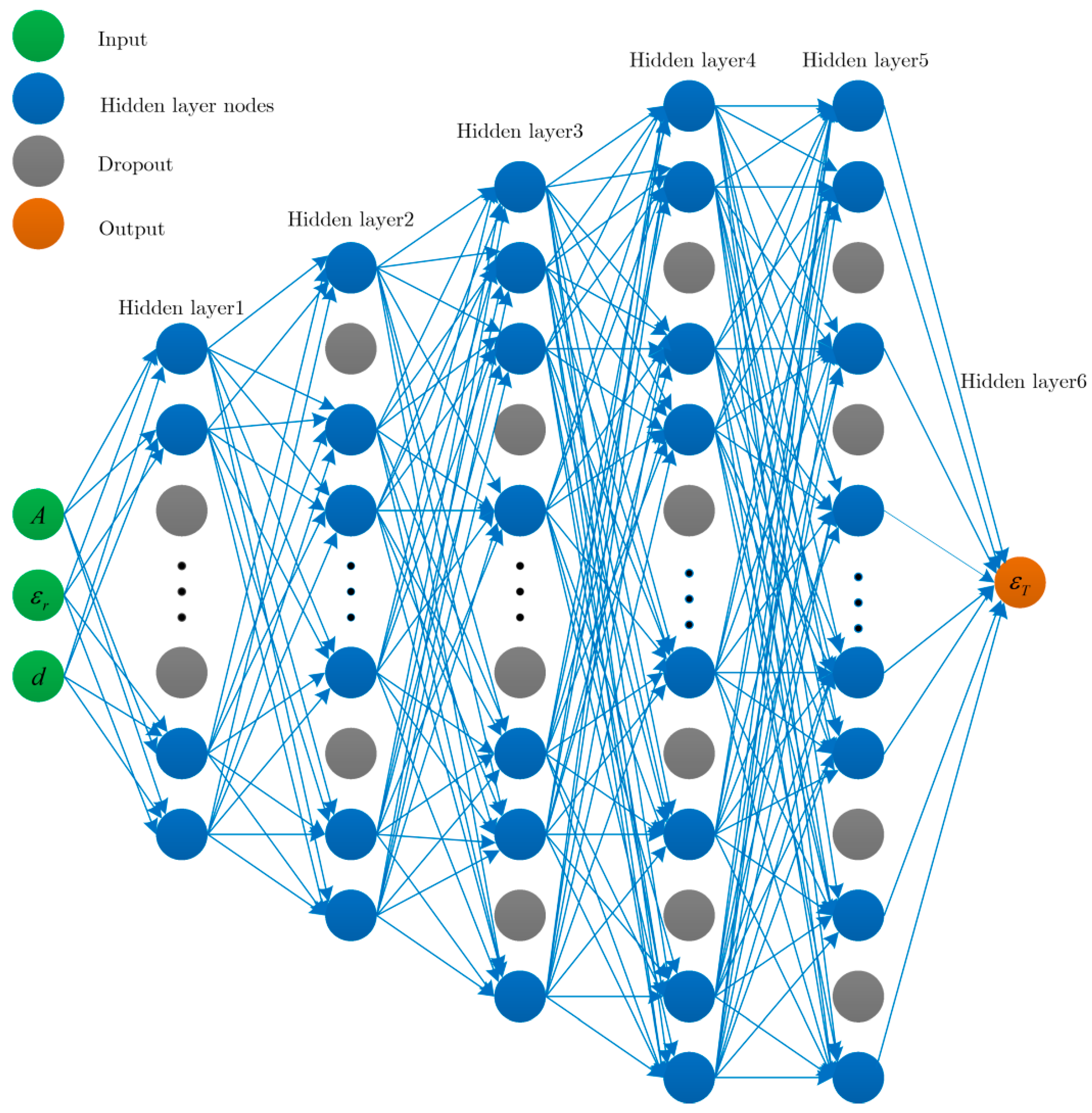
Figure 6.
Layered media model structure diagram.
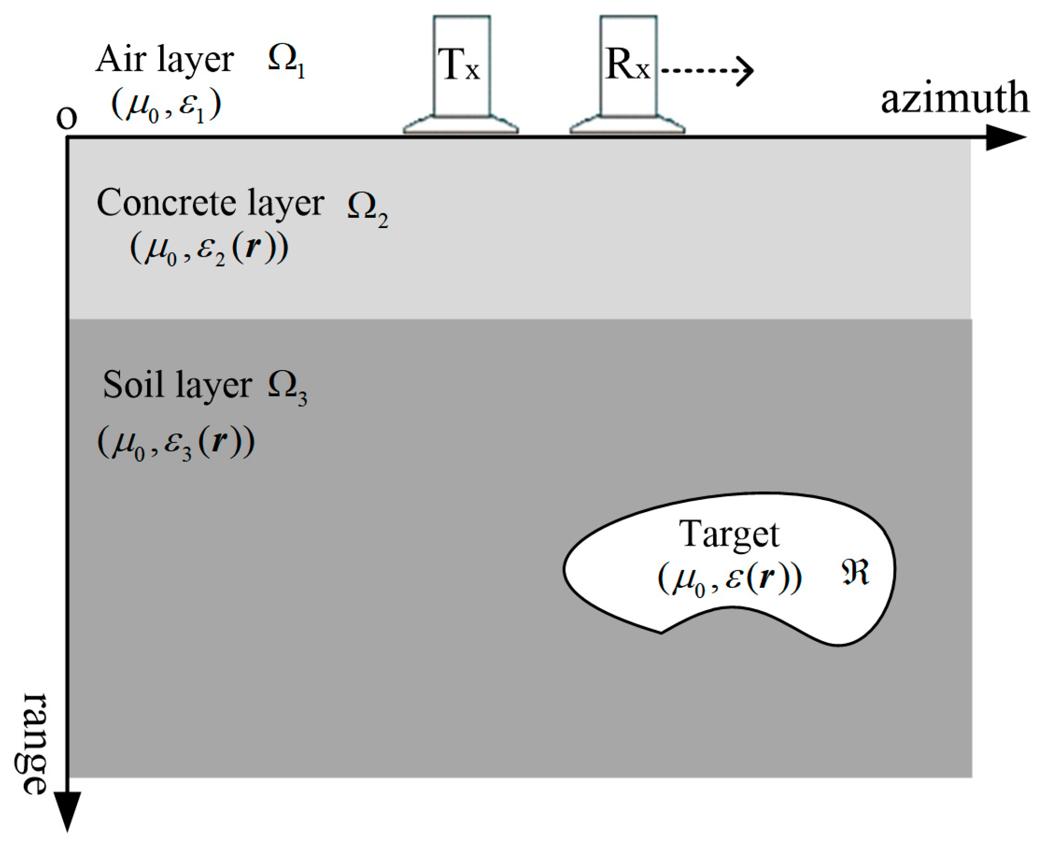
Figure 7.
GPR B-SCAN image feature curve detection results. (a) Air-filled target; (b) fitted air-filled target feature curve; (c) water-filled target; (d) fitted water-filled target feature curve.
Figure 7.
GPR B-SCAN image feature curve detection results. (a) Air-filled target; (b) fitted air-filled target feature curve; (c) water-filled target; (d) fitted water-filled target feature curve.

Figure 8.
Calculation results of .
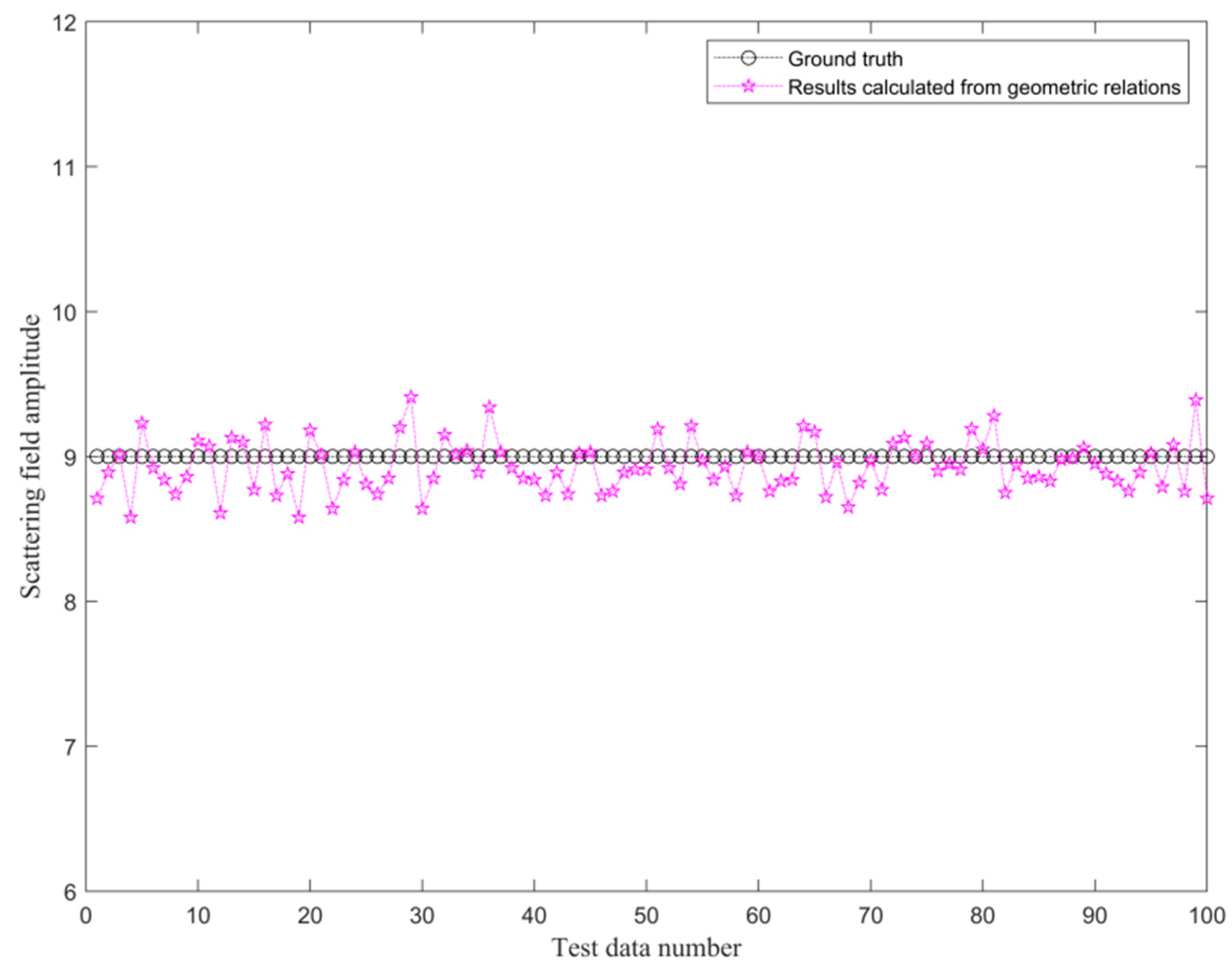
Figure 9.
GPR simulation data in a single-layer background medium for training regression networks. (a) The MSE loss of training data; (b) the MSE loss of validation data.
Figure 9.
GPR simulation data in a single-layer background medium for training regression networks. (a) The MSE loss of training data; (b) the MSE loss of validation data.
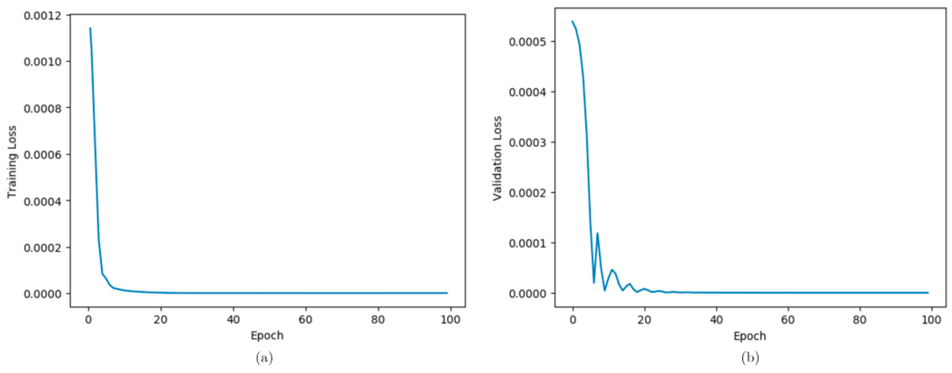
Figure 10.
Results of estimating in single-layer media. (a) Air-filled target; (b) water-filled target.
Figure 10.
Results of estimating in single-layer media. (a) Air-filled target; (b) water-filled target.
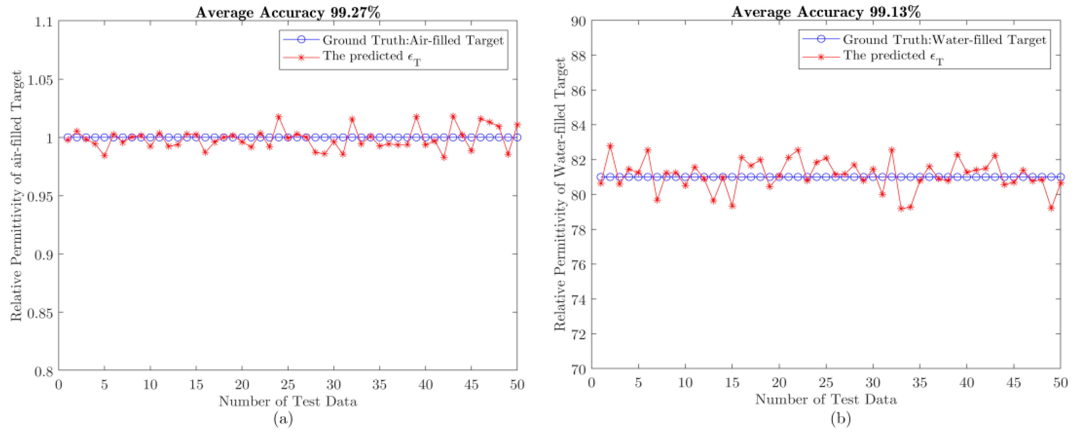
Figure 11.
Hyperbolic fitting results in GPR B-SCAN images. (a) One air-filled target; (b) one water-filled target; (c) two air-filled targets; (d) two water-filled targets.
Figure 11.
Hyperbolic fitting results in GPR B-SCAN images. (a) One air-filled target; (b) one water-filled target; (c) two air-filled targets; (d) two water-filled targets.

Figure 12.
The result of calculating the mean of .
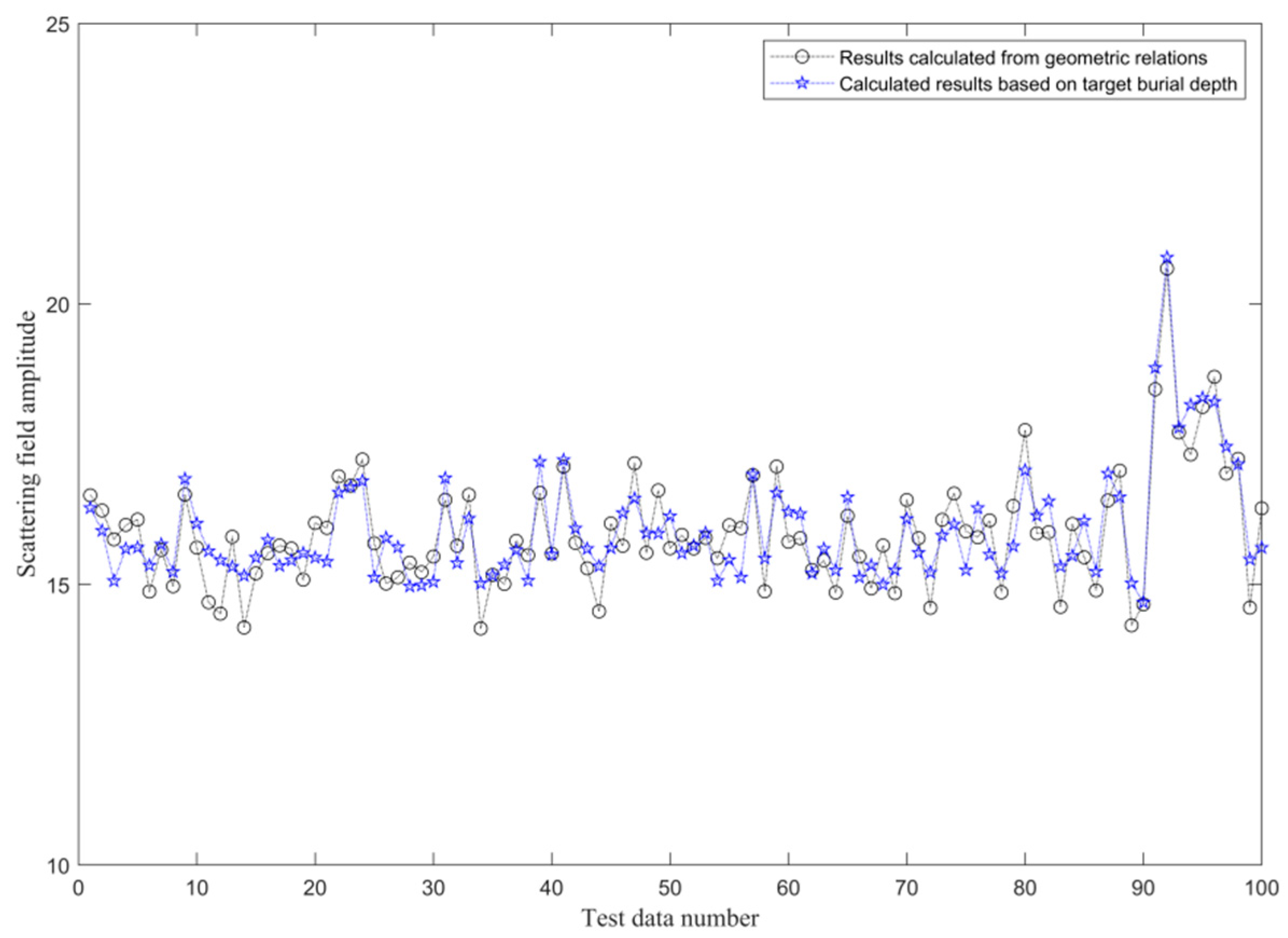
Figure 13.
GPR simulation data under the layered background medium for training regression networks. (a) The MSE loss of training data; (b) the MSE loss of validation data.
Figure 13.
GPR simulation data under the layered background medium for training regression networks. (a) The MSE loss of training data; (b) the MSE loss of validation data.

Figure 14.
Results of estimating in layered media. (a) Air-filled target; (b) water-filled target.
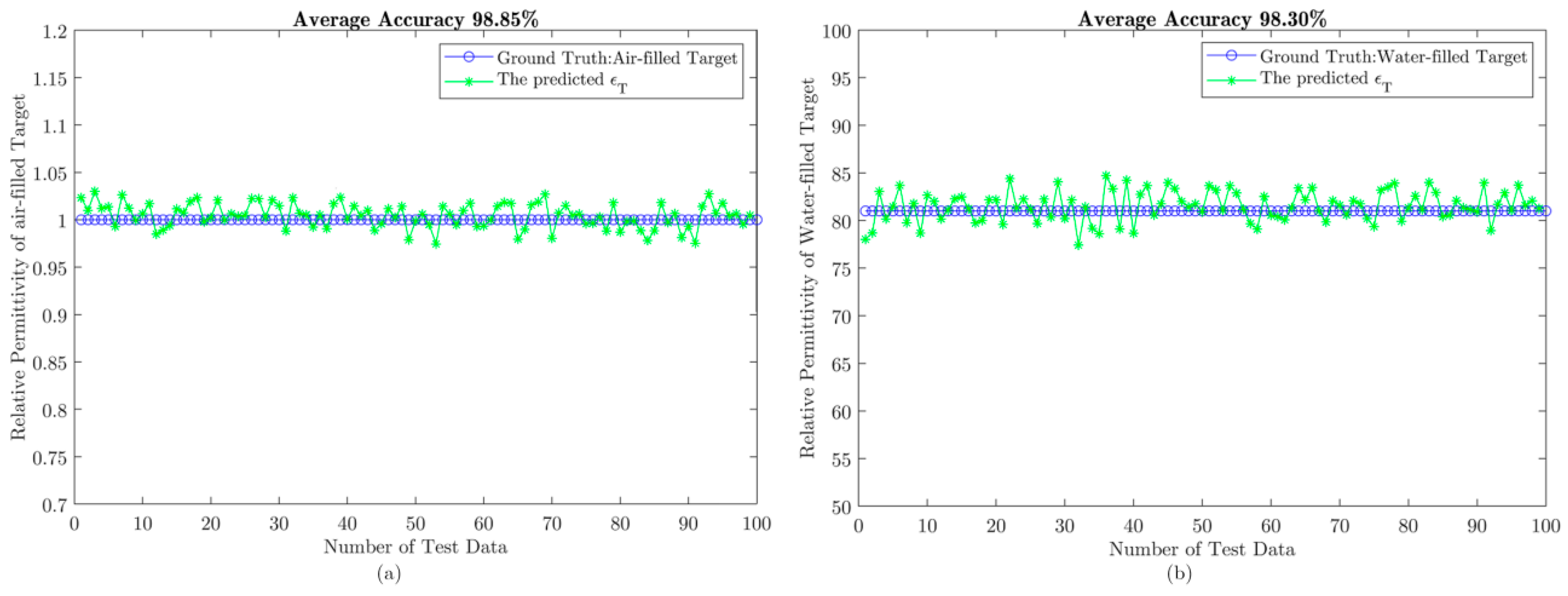
Figure 15.
Statistical results of for parameters and under different deviation ranges.

Figure 16.
GPR field data collection. (a) LAUREL radar physical picture; (b) the rainwater pipe under the manhole cover; (c) GPR B-SCAN image.
Figure 16.
GPR field data collection. (a) LAUREL radar physical picture; (b) the rainwater pipe under the manhole cover; (c) GPR B-SCAN image.
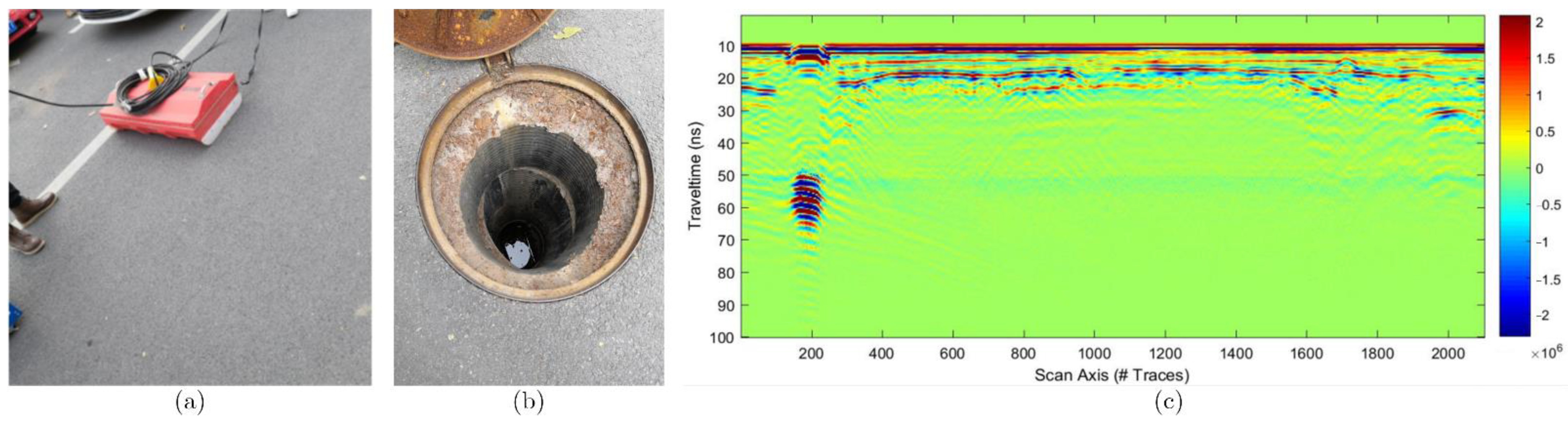
Figure 17.
The predicted results on the field data set.


Table 1.
Details of the DNN.
| Layer | Ouput_Dim | Layer Details |
|---|---|---|
| Hidden layer 1 | 64 | Input_dim: 3 Activation: Relu Dropout: 0.2 |
| Hidden layer 2 | 128 | Input_dim: 3 Activation: Relu Dropout: 0.2 |
| Hidden layer 3 | 256 | Input_dim: 3 Activation: Relu Dropout: 0.2 |
| Hidden layer 4 | 512 | Input_dim: 3 Activation: Relu Dropout: 0.3 |
| Hidden layer 5 | 512 | Input_dim: 3 Activation: Relu Dropout: 0.3 |
| Hidden layer 6 | 1 | — |
Table 2.
Comparison with FWI.
| Index | Average Accuracy | Estimated Range | Time Consuming | |
|---|---|---|---|---|
| Algorithm | ||||
| FWI-based | 89.13% | 0.86–1.18 | 2820 s | |
| DNN-based | 95.52% | 0.93–1.05 | 0.023 s | |
Publisher’s Note: MDPI stays neutral with regard to jurisdictional claims in published maps and institutional affiliations. |
© 2022 by the authors. Licensee MDPI, Basel, Switzerland. This article is an open access article distributed under the terms and conditions of the Creative Commons Attribution (CC BY) license (https://creativecommons.org/licenses/by/4.0/).
Share and Cite
MDPI and ACS Style
Wang, H.; Ouyang, S.; Liu, Q.; Liao, K.; Zhou, L. Deep-Learning-Based Method for Estimating Permittivity of Ground-Penetrating Radar Targets. Remote Sens. 2022, 14, 4293. https://doi.org/10.3390/rs14174293
AMA Style
Wang H, Ouyang S, Liu Q, Liao K, Zhou L. Deep-Learning-Based Method for Estimating Permittivity of Ground-Penetrating Radar Targets. Remote Sensing. 2022; 14(17):4293. https://doi.org/10.3390/rs14174293
Chicago/Turabian StyleWang, Hui, Shan Ouyang, Qinghua Liu, Kefei Liao, and Lijun Zhou. 2022. "Deep-Learning-Based Method for Estimating Permittivity of Ground-Penetrating Radar Targets" Remote Sensing 14, no. 17: 4293. https://doi.org/10.3390/rs14174293
Note that from the first issue of 2016, this journal uses article numbers instead of page numbers. See further details here.