
An eLoran Signal Cycle Identification Method Based on Joint Time–Frequency Domain
by
 , , and
Wenhe Yan
1,2,3,* ,
,
Ming Dong
4,
Shifeng Li
1,2,3,
Chaozhong Yang
1,3,
Jiangbin Yuan
1,3,
Zhaopeng Hu
1,3 and
Yu Hua
1,2,3 1
National Time Service Center, Chinese Academy of Sciences, Xi’an 710600, China
2
University of Chinese Academy of Sciences, Beijing 100049, China
3
Key Laboratory of Precise Positioning and Timing Technology, Chinese Academy of Sciences, Xi’an 710600, China
4
Beijing Institute of Tracking and Telecommunications Technology, Beijing 100094, China
*
Author to whom correspondence should be addressed.
Remote Sens. 2022, 14(2), 250; https://doi.org/10.3390/rs14020250
Submission received: 27 November 2021
/
Revised: 3 January 2022
/
Accepted: 4 January 2022
/
Published: 6 January 2022
(This article belongs to the Special Issue Remote Sensing in Navigation: State-of-the-Art)
Abstract
:The eLoran system is an international standardized positioning, navigation, and timing service system, which can complement global navigation satellite systems to cope with navigation and timing warfare. The eLoran receiver measures time-of-arrival (TOA) through cycle identification, which is key in determining timing and positioning accuracy. However, noise and skywave interference can cause cycle identification errors, resulting in TOA-measurement errors that are integral multiples of 10 μs. Therefore, this article proposes a cycle identification method in the joint time–frequency domain. Based on the spectrum-division method to determine the cycle identification range, the time–domain peak-to-peak ratio and waveform matching are used for accurate cycle identification. The performance of the method is analyzed via simulation. When the signal-to-noise ratio (SNR) ≥ 0 dB and skywave-to-groundwave ratio (SGR) ≤ 23 dB, the success rate of cycle identification is 100%; when SNR ≥ −13 dB and SGR ≤ 23 dB, the success rate exceeds 75%. To verify its practicability, the method was implemented in the eLoran receiver and tested at three test sites within 1000 km using actual signals emitted by an eLoran system. The results show that the method has a high identification probability and can be used in modern eLoran receivers to improve TOA-measurement accuracy.
1. Introduction
With continuous improvements in informatization, positioning, navigation, and timing (PNT) systems have become indispensable for social development and modern national defense infrastructure, reflecting a country’s international status and comprehensive strength [1,2,3]. Although global navigation satellite systems (GNSS) are currently the most widely used type of PNT system, GNSS signals are weak, ineffective at penetration, and susceptible to interference. GNSS systems are thus not suitable for applications in special scenarios, including underground, underwater, and indoors [4,5,6]. Therefore, relying solely on GNSS involves serious risks.
The enhanced long-range navigation (eLoran) system evolved from the Loran-C system. It is an internationally standardized medium and a long-range land-based radio system [7,8]. It can satisfy the requirements of PNT applications in most fields in terms of accuracy, reliability, and continuity. It can also provide a time service better than 100 ns and a position service of 20 m after differential correction [7,9]. When a GNSS signal is unavailable, the eLoran system can be used as a backup, which reduces the risk caused by relying on GNSS; this also allows for coping with timing warfare and navigation warfare in modern war [10,11,12]. Therefore, several countries are developing and upgrading their eLoran systems. In August 2019, the US Department of Defense (DoD) released a report titled “Strategy for the DoD Positioning, Navigation, and Timing (PNT) Enterprise—ensuring a US military PNT advantage”, which stated that Loran-C should be listed as the PNT source, second only to GNSS [13]. China also planned to build three eLoran stations in its western region in 2018 to achieve national coverage of eLoran signals together with the existing eLoran system [14]. The construction of the three stations officially started in 2020. Russia has developed a new land-based radio navigation system called “Scorpion,” with the aim of achieving balanced development of satellite-based and land-based PNT systems [15]. South Korea began to develop and deploy its own eLoran system in 2013 due to the deliberate interference of North Korea on its GPS; in 2021, it was announced that the developed eLoran system had commenced operation [16,17]. Although eLoran can be used as to supplement GNSS, the current global eLoran application technology is not sufficiently advanced. Compared with those of GNSS, the accuracy and reliability of the application terminals of eLoran remain inadequate. Therefore, eLoran cannot fully satisfy the requirements of users of PNT services.
The eLoran signal is a long-wave (LW) signal with a frequency of 100 kHz. According to the propagation theory of this frequency band, the eLoran signal is a composite wave consisting of a groundwave signal and a skywave signal [18,19]. The eLoran receiver provides timing and positioning services by measuring the time-of-arrival (TOA) of the groundwave signal in the composite wave. Cycle identification is an important task for the eLoran receiver. It involves correctly identifying the standard zero-crossing (SZC) of the eLoran ground wave signal to measure the TOA [20,21]. Because the SZC point of the eLoran signal has no prominent characteristics, the skywave interference (SWI) signal generated by ionospheric reflection arrives at the receiver a certain cycle after the groundwave signal does, which affects the cycle identification result. The carrier frequency of the eLoran signal is 100 kHz. If the cycle identification is incorrect, it produces errors in the TOA measurement that are integral multiples of 10 μs; this severely affects the positioning and timing accuracy. Moreover, the cycle identification is affected by not only SWI but also noise [19,21]. As the receiving distance increases, the signal amplitude decreases, and the signal-to-noise ratio (SNR) deteriorates, which considerably affects the accuracy of cycle identification.
To solve the problems with eLoran signal cycle identification, in [22], a delayed-addition method was proposed, which uses an eLoran pulse signal to subtract the signal after a certain time delay to achieve phase inversion of the signal at 30 μs. This is achieved by detecting the position of the phase inversion point to realize SZC detection. However, this method exhibits poor anti-noise performance, and SWI causes the result to have multiple phase-reversal points. In [23], the polarity-judgment method was proposed, in which a positive zero crossing is selected, and the signals are accumulated at , , and for a long duration. If the accumulated result exceeds the threshold, then is the SZC; otherwise, t is moved forward or backward by 10 μs, and the process is repeated. This method is time-consuming, and it is challenging to find a suitable threshold. In [24], a cross-correlation method was proposed, which uses the local standard eLoran signal to correlate with the received signal and calculates the SZC by detecting the maximum value of the correlation result. This method is only applicable to situations where the amplitude of the groundwave is greater than that of the skywave. In [25], the peak-to-peak ratio detection method was proposed, in which the ratio of the signal amplitude at to that at is calculated. If the ratio is close to a standard value, then it is considered as the standard zero-crossing. However, this method is affected by the skywave and noise, which can produce multiple values, resulting in identification errors. In [26], a delay-locked loop (DLL) method was proposed, wherein the lag envelope is subtracted from the advance envelope to obtain the envelope with a peak point of 0, and the SZC is obtained by detecting the zero point of the envelope. This method uses the peak value of the envelope of the ground wave signal; thus, the premise of the method is to eliminate the skywave. Bian and Last [27] proposed the method of spectrum division to estimate the starting positions of the skywave and groundwave to realize cycle identification. However, this method has a poor estimation resolution under the condition of low SNR. Other researchers have proposed the autoregressive moving average model (ARMA) and multiple signal classification algorithm (MUSIC) methods based on spectrum division to improve the resolution of estimation; however, these methods are not only difficult to implement but are suffer from inaccurate parameter estimation [28,29,30].
Based on the foregoing account of previous research, cycle identification methods can be divided into two types: signal-waveform reconstruction and parameter estimation. In signal-waveform reconstruction methods, cycle identification is realized by constructing the characteristics of SZC. This method can fail under low SNR, and multiple identification results under SWI can be produced; hence, relying solely on this method is hazardous. The parameter-estimation method is mainly based on spectrum-division theory, and the estimation error is high at under SNR. Therefore, a single-cycle identification method is unreliable and has poor anti-noise ability. Hence, this paper proposes a joint time–frequency domain method to realize cycle identification of an eLoran signal. On the basis of improving SNR and repairing the envelope using a digital bandpass filter (BPF) and linear digital averaging (LDA), the range of SZCs is determined via spectral division in the frequency domain, and accurate identification of the SZC is realized through peak-to-peak ratio detection and waveform matching. In this study, the performance of the cycle identification method was simulated, and the method was verified via field testing. The methods, findings, and conclusions of this study are presented in the following sections.
The rest of the paper is organized as follows. Section 2 presents the format of the eLoran signal and skywave interference and describes the impact of the skywave interference on cycle identification. The principle and model of the joint cycle identification method in the time–frequency domain are also described. Section 3 describes the verification of the effectiveness of the cycle identification method and the simulation of the performance of the period identification method under different signal-to-noise ratios (SNRs) and skywave interference. The eLoran signals actually received in three places were used to verify the cycle identification method, and the test results were verified. Section 4 summarizes the main conclusions of this study.
2. Materials and Methods
In this section, we first describe the single-pulse signal format and pulse group signal characteristics broadcast by the eLoran system. Second, along with the propagation channel of the eLoran signal, the influence of SWI on cycle identification is analyzed. Finally, the principle of the cycle identification method based on the joint time–frequency domain is presented, and the key parameters of the algorithm are discussed.
2.1. eLoran Signal Format
The working frequency allocated to the eLoran system by the International Telecommunication Union (ITU) is 100 kHz, and the bandwidth is 90–110 kHz. It is required that 99% of the transmitted signal energy be concentrated within the specified bandwidth. At the beginning of the system design, the center frequency, signal-waveform, transmission period, and data-modulation mode of the transmission signal are considered comprehensively, and the existing pulse-phase signal system is formed. The single-pulse signal waveform of the eLoran system is defined by the United States Coast Guard (USCG) as [31].
where is time (), A is a normalization constant related to the peak amplitude, is the carrier frequency of 100 kHz, is the envelope-to-cycle difference (ECD) (), and is the phase-code parameter, which is 0 for positive phase-coded (PC) pulses and for negative PC pulses. The eLoran pulse signal is generated according to Equation (1). The time–domain and frequency–domain characteristics of a single eLoran signal are shown in Figure 1. It can be seen that the leading edge of the signal first rises rapidly, reaching a peak at 65 μs, and then falls rapidly.
The eLoran system can be a timing station or a navigation chain. The timing station generally has only one master station, and the navigation chain generally consists of one master station and two to five secondary stations. The master station is generally represented by M, and the secondary station is represented by letters such as W, X, Y, and Z. To distinguish between the signals of the master and secondary stations, each group of the master station transmits nine eLoran pulse signals. The interval between the first eight pulse signals is 1 ms, and that between the eighth and ninth pulse signals is 2 ms. The secondary station transmits only eight pulses. The pulse-group signals of the master and secondary stations are shown in Figure 2.
The interval between the eLoran pulse groups is called the group-repetition interval (GRI). The GRI cycle range is defined as 40,000–99,990 μs, with a resolution of 10 μs. The eLoran system continuously emits pulse-group signals according to its own GRI. The phase-code cycles are listed in Table 1. The two code cycles are alternately modulated with the signal; “+” indicates a phase code of 0 radians, and “−” indicates a phase code of π radians. Each pulse signal in the eLoran pulse group of the master and secondary stations is phase-coded. The third to eighth pulse signals of each pulse group are used for the Loran data channel (LDC), which is used for transmitting system status, time information, etc. The modulation mode adopts Eurofix data-modulation technology [32,33].
In the eLoran system, the sixth zero crossing (30 μs) of the first pulse of the pulse group is designated as the SZC. The SZC has two key functions: (i) it serves as the pulse-time reference (PTR) for measuring the signal specification of the eLoran broadcasting station; (ii) it allows the eLoran receiver to measure the TOA of the signal to realize high-precision positioning and timing.
2.2. Skywave Interference and Cycle Identification
The eLoran signal belongs to an LW frequency band with a carrier frequency of 100 kHz. According to the propagation theory of this frequency band, the eLoran signal mainly reaches the receiving point through two paths: (i) as a groundwave signal (surface wave) transmitted along the surface of the Earth, and (ii) as a skywave signal (space wave) produced by one or more reflections between the ionosphere and the ground when the signal is projected to the ionosphere at a certain elevation angle. Generally, only one-hop skywave is considered for receiving points with a receiving distance of less than 2000 km [34]. The propagation path of the eLoran signal is shown in Figure 3.
The composite wave comprising the eLoran groundwave and skywave signals received in space can be expressed as:
where is the standard eLoran signal with a normalized amplitude, is the amplitude of the groundwave signal, is the amplitude of the skywave signal, is the delay difference of the skywave relative to the groundwave, and is noise.
The skywave-to-groundwave ratio (SGR) is the amplitude ratio of the skywave relative to the groundwave, expressed as:
The time-delay difference of the skywave relative to the groundwave is expressed as:
where and are the propagation delays of the groundwave and skywave, respectively.
Figure 4 shows two typical eLoran received-signal waveforms. The first case is where the phase difference is 0° due to the time delay of the skywave relative to the groundwave, which increases the amplitude of the composite signal. The second case is where the phase difference is 180° due to the time delay of the skywave relative to the groundwave, which reduces the amplitude of the composite signal. In both cases, the groundwave is distorted, and the signal amplitude exhibits two extremes. This significantly affects the cycle identification result of the eLoran groundwave.
Cycle identification is the process of finding the SZC of the first pulse of the groundwave after the eLoran pulse acquisition. Ideally, only the pure groundwave signal is received, and the SZC can be detected by measuring the peak value (65 μs) of the eLoran groundwave envelope. However, the skywave is generated due to reflection from the ionosphere, and it always arrives at the receiver a certain cycle after the groundwave does. Therefore, the eLoran groundwave signal is susceptible to interference by the skywave delay [21,35]. According to the minimum receiver performance standards for marine eLoran receiving equipment issued by the Radio Technical Commission for Maritime Services (RTCM), the time delay range of the skywave relative to the groundwave is 37.5–1500 μs, and the amplitude ratio SGR of the skywave relative to the groundwave is 12–26 dB [36]. Therefore, to consider both the stability and the SNR, the positive zero crossing (30 μs) in the third week is usually selected as the SZC [37].
2.3. Time–Frequency Domain Cycle Identification Method
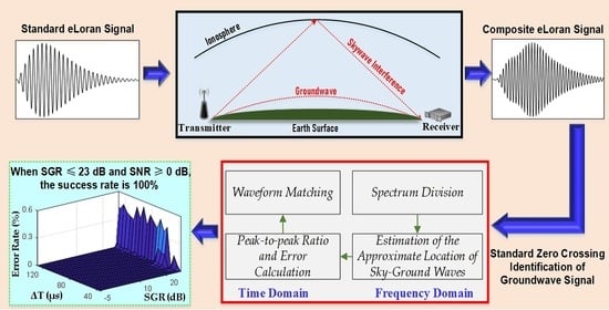
Because the phase of the first pulse signal in the eLoran pulse group is “+” and there is no data modulation, cycle identification is performed using the first pulse in the eLoran pulse group. To overcome the low identification probability and poor anti-interference ability of existing cycle identification methods, we propose a time–frequency domain method to identify the SZC of the eLoran signal. The frequency–domain method uses spectrum division to estimate the approximate starting positions of the skywave and groundwave, which is also the cycle identification range; the time–domain method uses the peak-to-peak ratio and waveform matching to determine the SZC accurately. The specific implementation process of the method is shown in Figure 5. We assume that the received signal is as follows:
where is the amplitude ratio of the skywave to the groundwave, is the delay difference of the groundwave relative to the local standard eLoran signal, is the delay difference of the skywave relative to the local standard eLoran signal, is the delay difference of the eLoran skywave relative to groundwave, and is noise in the signal.
2.3.1. Digital Bandpass Filtering and Linear Digital Average
Before the cycle identification, the received signal must be filtered to suppress noise and interference and improve the SNR, to obtain relatively clean composite signals of the groundwave and skywave.
From the eLoran frequency band, the cycle identification results are mainly affected by noise and continuous wave interference (CWI). We used BPFs to suppress out-of-band noise and interference. The BPF includes a Hamming window with a bandwidth of 30 kHz and an order of 128, and its out-of-band suppression capability can exceed 30 dB. The bandpass-filtered signal is:
where is the residual noise in the bandpass-filtered signal.
In the eLoran frequency band, the cycle identification results are mainly affected by noise. After bandpass-filtering, we used LDA to suppress in-band noise, which not only suppresses the noise and improves the SNR of the received signal, but also repairs the eLoran signal and reduces the signal distortion. The LDA is the cumulative average processing of the received signal for M times according to the GRI cycle. Assuming that there are M signals with a length equal to the GRI, the LDA result can be expressed as:
where is the residual noise in the signal after LDA.
When the number of LDA is M, the gain of the SNR can be increased by . We chose the linear digital average of M = 64 to ensure that the SNR of the signal can be improved by 18 dB. A relatively clean composite signal with a length equal to the GRI can be obtained using the linear digital average. The cycle identification method in the time–frequency domain was subsequently used to identify the SZC.
2.3.2. Spectrum Division in Frequency Domain
The fast Fourier transform (FFT) was used to obtain the signal spectrum after LDA, and the approximate starting positions of the skywave and groundwave were determined via spectrum division. The FFT of is:
where is the FFT result of the eLoran signal and is the FFT result of the noise.
The spectrum-division method, proposed by Bian and Last, is based on high-resolution time delay estimation under multipath conditions [38]. When Equation (8) is divided by the Fourier transform of the standard eLoran signal, the spectrum-division result is:
where is the amplitude ratio of the received groundwave signal to the standard signal, and is the result of dividing the noise by the standard eLoran signal. According to Euler’s formula:
The Equation (10) is a sine wave with variable , and the frequency of sine wave is . Therefore, the result of the spectrum division of the received signal in Equation (9) becomes an estimate of two continuous wave frequencies and . The amplitude ratio is the ratio of the amplitudes of the two continuous waves.
Figure 6 shows the results of spectrum division without noise and with SNR = 5 dB. The waveform of the spectrum division result in the absence of noise was composed of continuous waves formed by different time delays, which is consistent with the theoretical analysis. However, after noise was added, the out-of-band noise was amplified by the spectrum division, which increased the out-of-band noise of the eLoran signal and reduced the SNR sharply. The waveform of the two continuous waves was difficult to distinguish. The Hamming window offered the advantages of low side-lobe attenuation and strong out-of-band suppression. Therefore, a Hamming window with a bandwidth of 50 kHz was selected to suppress out-of-band noise in the spectrum-division results. After windowing, Equation (9) became:
where is the window function.
Finally, the inverse fast Fourier transform (IFFT) was used to estimate the parameters of the skywave and groundwave [39,40]. The IFFT of Equation (11) is:
where represents the IFFT.
It can be seen from Equation (12) that is the impulse response function resulting from the IFFT of the synthetic signals of the groundwave and skywave. The time delays and and amplitude ratio can be estimated by detecting the time–domain pulse peak value after IFFT. However, the time delay only represents the approximate starting positions of the skywave and groundwave, and the estimated position has a bias; thus, the SZC had to be further determined in the time domain.
2.3.3. Peak-to-Peak Ratio and Waveform Matching in Time Domain
The result of spectrum division determined the starting position range of the groundwave and the skywave in the composite wave. Therefore, we determined the position of the SZC using the peak-to-peak ratio and waveform methods in the time domain.
The peak-to-peak ratio method first determined all positive zero crossing points () in the range of and then calculated the ratio of the positive peak value in the next week () and the previous week () of each positive zero crossing. If the calculated peak-to-peak ratio was close to the peak-to-peak ratio of the standard eLoran signal a certain range, then it was considered as a possible SZC [23]. The theoretical formula for calculating the peak-to-peak ratio is:
The peak-to-peak ratios of positive zero crossings in the theoretical calculation are displayed in Table 2. It can be seen that the peak-to-peak ratio at 30 μs was 1.5338.
The peak-to-peak ratios of all positive zero crossings in the range after LDA are calculated first; then, the errors of the peak-to-peak ratios are calculated:
where is the peak-to-peak ratio of zero crossings, and is the number of zero crossings.
Because the eLoran signal was distorted during propagation and signal processing, which can lead to deviations in the peak-to-peak ratios, when , we determined that the zero crossing was the closest to the SZC. Thus, the peak-to-peak ratio results contained multiple possible SZCs. Therefore, we used waveform matching to calculate the root mean square (RMS) error between the received signal and the standard waveform over a cycle of time. The minimum value of the RMS error corresponded to the zero crossing to determine the SZC. The waveform-matching calculation formula was as follows:
where is the standard eLoran signal, is the received eLoran signal, and is the waveform-matching range. To prevent the influence of SWI, we adopted a waveform matching range of 10–50 μs. Therefore, when was the smallest, the corresponding n was the SZC.
3. Results
In this section, we analyze the effectiveness and performance of the joint time–frequency cycle identification method through simulation. Then, we validate the cycle identification method by receiving actual eLoran signals at different locations.
3.1. Validation of Cycle Identification Method
To verify the effectiveness of the proposed method, we performed a simulation, the parameters of which were set as follows. The GRI of the eLoran signal generated by the simulation was 60 ms. After adding noise to the signal, the SNR of groundwave was −5 dB; the amplitude ratio of the skywave to the groundwave was SGR = 10 dB; the time-delay difference between the skywave and the groundwave was ; and the sampling rate of the simulation process signal was . The simulation results are shown in Figure 7.
As can be seen from Figure 7a, the composite wave of the skywave and groundwave generated in the simulation is submerged in noise, and the groundwave signal is severely distorted. Figure 7b presents the bandpass-filtered signal. It can be seen that although the noise in the signal is suppressed, the signal distortion is relatively large. Figure 7c shows the signal after LDA. It can be seen that the signal not only became cleaner, but the signal waveform also became complete through repair. The spectrum-division method was then used to obtain the initial positions of the groundwave and skywave on the linearly averaged signal, as shown in Figure 7d. The range of the SZC was observed to be 320–445. The results of calculating the peak-to-peak ratio errors of all zero crossings in the determined range are shown in Figure 7e. As observed, the peak-to-peak ratio errors of zero crossings 3 and 4 were less than 0.3. Waveform matching was performed on the two zero-crossing points, and the results are shown in Figure 7f,g. The waveform-matching coefficients of the two zero-crossings were calculated to be 0.0456621 and 0.1117095, respectively. Thus, zero crossing 3 was the SZC. The SZC determined using the cycle identification method was consistent with that set based on the simulation, which proves the effectiveness of the method.
3.2. Performance Analysis of Cycle Identification Method
Noise and SWI are the most important interference sources that affect cycle identification, and they are inevitable. According to the minimum performance standard for eLoran receivers, the requirements for an eLoran receiver to function normally were SNR ≥ −10 dB, SGR < 12 dB, and > 37.5 μs [36]. Therefore, to verify the performance of the proposed cycle identification method, we analyzed the skywave and groundwave parameter-estimation performance of the spectrum-division method and the probability of cycle identification based on the joint time–frequency domain under different SNRs.
We simulated the parameter-estimation performance of the spectrum-division method under SNR = 5, 0, and –10 dB. For SGR = 5–10 dB and = 37–150 μs, the amplitude-ratio error and delay-difference error after spectrum estimation are shown in Figure 8.
Figure 8 shows that with a decrease in SNR, the estimation error of the time-delay difference and the amplitude ratio of the skywave to the groundwave based on the spectrum-division method increased. When SNR = 5 dB, the amplitude-ratio estimation error was less than 1 dB, and the delay-difference estimation error was less than 2 μs. When SNR = 0 dB, the amplitude-ratio estimation error was less than 1 dB, and the delay-difference estimation error was less than 10 μs. When SNR = −10 dB, the amplitude-ratio estimation error was less than 2 dB, and the delay-difference estimation error was less than 10 μs in most cases; however, when > 50 μs and SGR < −3 dB, the delay-difference estimation error was greater than 10 μs. In the actual received signal, the SNR may deteriorate, resulting in a greater estimation error in the delay difference. Therefore, based on the simulation results, the spectrum-division method cannot be used for complete cycle identification; more accurate cycle identification based on spectrum division using the time–domain method is necessary. To address the large estimation error of the spectrum-division method under a low SNR, we proposed a cycle identification method based on the combined time–frequency domain. Through spectral division, we further improved the accuracy of cycle identification in the time domain.
We simulated the parameter estimation performance of the cycle identification method under SNR = 0, −5, −10, and −13 dB. Figure 9 shows the error rate of cycle identification when SGR = 5–10 dB and = 37–150 μs.
The simulation results in Figure 9 show that when SGR ≤ 23 dB and SNR ≥ 0 dB, the success rate of cycle identification was 100%. When SGR ≤ 23 dB and SNR ≥ −10 dB, the success rate was better than 75%. When SGR ≤ 23 dB and SNR ≥ −13 dB, the success rate was better than 55%. The cycle identification was mainly affected by the relative amplitudes of the skywave and groundwave, especially under a low SNR. Although the success rate of cycle identification decreased with an increase in SGR, accurate cycle identification could be achieved via multiple cycle identification calculations. Therefore, the-simulation results showed that the proposed cycle identification method is effective and offers a high identification probability.
3.3. Experimental Verification of Cycle Identification Method
We validated the cycle identification method with actual signals transmitted by a real eLoran system. The test scheme is shown in Figure 10. The eLoran receiver obtains the signal transmitted by the eLoran station through the antenna, filters and amplifies the signal received by the radiofrequency (RF) unit, and converts it into a digital signal through the A/D chip. Next, the digital-signal-processing unit of the receiver captures the eLoran pulse-group signal to obtain the approximate position of the pulse signal. Finally, the proposed cycle identification method was used to identify the SZC of the first eLoran signal of the pulse group, and the identification result was saved in a computer. The digital signal processing in Figure 10 was completed on an FPGA chip. The test platform built according to the test scheme is shown in Figure 11.
The actual received signal is the signal emitted by the BPL timing system in China. The coordinates of the BPL timing system are Its GRI and transmission power are 60 ms and 2 MW, respectively. In July 2021, we selected three test sites within 1000 km of the system to receive actual signals. The coordinates, great circle distances, and electric-field strengths of the test sites are listed in Table 3.
The environments of the three selected test points were different. Test 1 was in a closed indoor environment, and Figure 12 shows the collected eLoran signal. It can be seen that although the receiving distance was short and there was only a groundwave signal, the signal was full of pulse interference. Test 2 was in the surrounding open environment, and Figure 13 shows the collected eLoran signal. It can be seen that there was SWI in the signal, which made the second half of the groundwave distorted. Test 3 was in a mountainous location at a large circle distance, and Figure 14 shows the collected eLoran signal. Not only was the skywave interference for this test strong, but the SNR was also very small, which made the groundwave signal severely distorted.
The results after the received signals of the three test sites were processed via the joint time–frequency domain cycle identification method are shown in Figure 15, Figure 16 and Figure 17. The number of cycles identified is 700. The peak-to-peak ratio errors of the three test points were 0.0124, 0.0676, and 0.0266, respectively, and the errors were all less than 0.3, meeting the peak-to-peak ratio evaluation conditions. However, as the distance increased, the dispersion of the eLoran signal became significant in the propagation process, leading to a larger standard deviation of the calculated result of the peak-to-peak ratio. The standard deviations of the peak-to-peak ratios were 0.0199, 0.0292, and 0.0938, but these results had no influence on the evaluation of the peak-to-peak ratio. The cycle identification results of the actual signals showed very high cycle identification success rates of tests 1 and 2 and only one identification error at test point 1. Although test point 3 was in a far-off mountainous area, the success rate of cycle identification for this test reached 72.86%. Comparing the experimental results with the simulation results, it can be seen that the cycle identification success rate of the actual measurement results is slightly worse. The main reason is that the actual eLoran signal received contains pulse interference, continuous wave interference and other interference, which would cause the quality of the eLoran signal to deteriorate and affect the success rate of cycle identification. In practical applications, accurate cycle identification can be achieved through multiple identification calculations. Therefore, the experimental test fully verifies the practicality of the proposed joint time–frequency domain eLoran cycle identification method.
4. Discussion
As an important part of the PNT system, the eLoran system can form a powerful supplement and backup to GNSS. Therefore, many countries are developing and improving eLoran systems to improve the service capabilities of the national PNT systems. Compared with GNSS, the accuracy and reliability of the eLoran system needs to be improved. Cycle identification is a key factor in determining the positioning and timing accuracy of eLoran receivers. However, due to noise in the space and the SWI caused by the signal propagation channel, the cycle identification success rate in the eLoran receiver is affected. The existing methods are poor in reliability and anti-interference; thus, this paper proposes a joint time–frequency domain cycle identification method. After the cycle identification range was determined by the spectrum division method, the peak-to-peak ratio and the waveform matching method were used to determine the accurate SZC, which can improve the success rate of cycle identification.
Firstly, based on the analysis of the propagation channel and interference characteristics of the eLoran signal, the principle of the joint time–frequency domain cycle identification method was given. The effectiveness of the method was verified by simulation, and the anti-noise and SWI performance of the method was analyzed. Simulation results showed that this method had a high success rate of cycle identification. When SNR ≥ 0 and SGR ≤ 23 dB, the success rate of cycle identification was 100%; when SNR ≥ −10 and SGR ≤ 23 dB, the success rate of cycle identification was greater than 75%; when SNR ≥ −13 and SGR ≤ 23 dB, the success rate of cycle identification was greater than 55%. When the success rate of the current cycle identification method reached 100%, the delay-locked loop method required SNR ≥ 20 dB, the waveform matching method required SNR ≥ 23 dB, and the delayed-addition method required SNR ≥ 24 dB. Although the performance of these methods can be improved by 10–18 dB after filtering, these methods can only meet the requirements under the condition of SGR ≤ 6 dB. Obviously, the cycle identification method proposed in this paper was better than the single cycle identification method for a combination of noise and skywave interference.
Finally, we applied the cycle identification method to the developed eLoran receiver and receive actual signals within 1000 km for testing. The test results show that under the condition of high SNR, the cycle identification success rate can reach 100%. Even in the 862.5-km mountain test environment, the method can achieve a 72.86% cycle recognition success rate. In practical applications, higher identification success rates can also be achieved by counting the results of multiple cycle identifications. Thus, the method has high engineering application value, and it is optimized for the design of the new eLoran navigation and timing receivers. It will be able to improve the accuracy of the application of modern eLoran systems, making it a more reliable backup for GNSS.
5. Conclusions
In this paper, a cycle identification method based on a joint time–frequency domain was proposed for the standard zero crossing detection of groundwave signals in eLoran positioning and timing receivers. We proved that this method has a good ability of anti-skywave and anti-noise detection and can address the limitation of poor detection performance of the current cycle identification method. This method also has a greater application potential, because it can be used for period identification as well as to obtain the time delay and amplitude of the skywave in the received signal, which is important for the receiver. In the future, we will use this method to separate the skywave and groundwave, in order to reduce the impact of skywave instability on the groundwave measurement. This can improve the TOA measurement accuracy of the eLoran signal and the information demodulation ability of the signal.
Author Contributions
Conceptualization, Y.H. and S.L.; methodology, W.Y. and M.D.; software, W.Y. and J.Y.; validation, W.Y., C.Y. and Z.H.; formal analysis, M.D.; investigation, M.D. and J.Y.; resources, S.L.; data curation, W.Y. and C.Y.; writing—original draft preparation, W.Y.; writing—review and editing, W.Y. and Y.H.; visualization, Z.H. and C.Y.; supervision, Y.H. and S.L.; project administration, W.Y. and C.Y.; funding acquisition, J.Y. All authors have read and agreed to the published version of the manuscript.
Funding
This work was supported by Chinese Academy of Sciences “Light of West China” Program (Grant No. XAB2018B21) and National Time Service Center “Youth Innovative Talent Project” (Grant No. Y917SC1S08).
Institutional Review Board Statement
Not applicable.
Informed Consent Statement
Not applicable.
Data Availability Statement
Restrictions apply to the availability of these data. The ownership of data belongs to the National Time Service Center (NTSC). These data can be available from the corresponding author with the permission of NTSC.
Acknowledgments
The authors would like to thank their colleagues for testing of the data provided in this manuscript. We are also very grateful to our reviewers who provided insight and expertise that greatly assisted the research.
Conflicts of Interest
The authors declare no conflict of interest.
References
- Xu, J.N. Analysis on underwater PNT system and key technologies. Navig. Position. Timing 2017, 4, 1–3. [Google Scholar] [CrossRef]
- Zhang, H.Y.; Xu, B.; Li, H.B.; Liao, D.Y.; Chen, H.Q. Prospects for development of loran-C navigation system for building up national comprehensive PNT system. J. Astronaut. Metrol. Meas. 2020, 40, 6–7. [Google Scholar] [CrossRef]
- Gao, Z.Z.; Ge, M.R.; Li, Y.; Shen, W.B.; Zhang, H.P.; Schuh, H. Railay irregularity measuring using rauch-tung-striebel smoothed multi-sensors fusion system: Quad-GNSS PPP, IMU, odometer, and track gauge. GPS Solut. 2018, 22, 22–36. [Google Scholar] [CrossRef]
- Di, Q.; Dan, B.; Sherman, L.; Per, E. Reliable location-based services from radio navigation systems. Sensors 2010, 10, 11369–11385. [Google Scholar] [CrossRef]
- Specht, M. Determination of navigation system positioning accuracy using the reliability method based on real measurements. Remote Sens. 2021, 13, 4424. [Google Scholar] [CrossRef]
- Krasuski, K.; Savchuk, S. Determination of the precise coordinates of the GPS reference station in of a GBAS system in the air transport. Commun. Sci. Lett. Univ. Zilina 2020, 22, 11–18. [Google Scholar] [CrossRef]
- Li, Y.; Hua, Y.; Yan, B.R.; Guo, W. Experimental study on a modified method for propagation delay of long wave signal. IEEE Antennas Wirel. Propag. Lett. 2019, 18, 1719. [Google Scholar] [CrossRef]
- Specht, C.; Weintrit, A.; Specht, M. A History of maritime radio-navigation positioning systems used in Poland. J. Navig. 2016, 69, 468–480. [Google Scholar] [CrossRef] [Green Version]
- Offermans, G.; Bartlett, S.; Schue, C. Providing a resilient timing and UTC service using eLoran in the United States. Navig. J. Inst. Navig. 2017, 64, 339–345. [Google Scholar] [CrossRef]
- Ren, S.H.; Lou, Y.L.; Yang, N.; Zheng, X.X.; Kang, S.L. Navigation warfare and its countermeasures. J. Navig. Pos. 2020, 8, 100–104. [Google Scholar] [CrossRef]
- Ge, Y.T.; Xu, L.L. Analysis on the disadvantage of American navigation and timing warfare. Aerodyn. Missile J. 2020, 6, 6–11. [Google Scholar] [CrossRef]
- Wang, X.Y.; Zhang, S.F.; Sun, X.W. The additional secondary phase correction system for AIS signals. Sensors 2017, 17, 736. [Google Scholar] [CrossRef] [Green Version]
- Strategy for the Department of Defense Positioning, Navigation and Timing (PNT) Enterprise—Ensuring a US Military PNT Advantage. Available online: https://rntfnd.org/wp-content/uploads/DoD-PNT-Strategy.pdf (accessed on 15 October 2021).
- Yan, W.H.; Zhao, K.J.; Li, S.F.; Wang, X.H.; Hua, Y. Precise loran-C signal acquisition based on envelope delay correlation method. Sensors 2020, 20, 2329. [Google Scholar] [CrossRef] [Green Version]
- About the Main Directions (Plan) of the Development of Radio Navigation CIS Member States for 2019–2024. Available online: https://rntfnd.org/wp-content/uploads/CIS-Russia-Radionav-Plan-2019-2024.pdf (accessed on 18 October 2021).
- Son, P.W.; Park, S.G.; Han, Y.; Seo, K. eLoran: Resilient positioning, navigation, and timing infrastructure in maritime areas. IEEE Access 2020, 8, 193708–193710. [Google Scholar] [CrossRef]
- Rhee, J.H.; Kim, S.; Son, P.W.; Seo, J. eLoran: Enhanced accuracy simulator for a future Korean nationwide eLoran system. IEEE Access 2021, 9, 115042–115045. [Google Scholar] [CrossRef]
- Zhou, L.L.; Yan, J.J.; Mu, Z.L.; Pu, Y.R.; Wang, Q.Q.; He, L.F. Field-strength variations of LF one-hop sky waves propagation in the earth-ionosphere waveguide at short ranges. IEEE Trans. Antennas Propag. 2021, 69, 3443–3445. [Google Scholar] [CrossRef]
- Last, J.D.; Farnworth, R.G.; Searle, M.D. Effect of skywave interference on the coverage of loran-C. IEE Proc. F-Radar Signal Process. 1992, 139, 306–312. [Google Scholar] [CrossRef]
- Zou, D.C.; Bian, Y.J.; Wu, H.T.; Su, J.F.; Li, Y. Digital algorithm realized with SOPC for cycle identification of Loran-C. J. Harbin Inst. Technol. 2005, 37, 1644–1646. [Google Scholar] [CrossRef]
- Fisher, A.J. Loran-C cycle identification in hard-limiting receivers. IEEE Trans. Aerosp. Electron. Syst. 2000, 36, 290–297. [Google Scholar] [CrossRef]
- Yan, Y.J.; Guo, Q. A novel signal search algorithm for loran-C receiver. Electron. Technol. 2010, 47, 20–21. [Google Scholar] [CrossRef]
- Yan, W.H.; Hua, Y.; Yuan, J.B.; Zhao, K.J.; Li, S.F. A ioint detection method of cycle-identification for loran-C signal. In Proceedings of the 2017 13th IEEE International Conference on Electronic Measurement & Instruments (ICEMI), Yangzhou, China, 20–22 October 2017. [Google Scholar] [CrossRef]
- Lin, H.Z.; Luo, B.F.; Hu, D.L.; Yang, Z.J. Algorithm of matching wave for cycle identification of LORAN-C. Ship Electron. Eng. 2008, 167, 81–83. [Google Scholar] [CrossRef]
- Sui, J.P.; Jin, X.Q.; Shu, D.L.; Ma, R.S. Improved Loran-C joint identification algorithm for sky-ground wave and cycle based on optimized envelope. Electron. Meas. Technol. 2020, 43, 115–119. [Google Scholar] [CrossRef]
- Li, S.F.; Gao, Y.Y.; Hua, Y. Joint cycle-identification method for Loran-C signal. J. Jiangsu Univ. 2014, 35, 547–551. [Google Scholar] [CrossRef]
- Bian, Y.; Last, J.D. Loran-C skywave delay estimation using eigen-decomposition techniques. eLectronics Lett. 1995, 31, 133–134. [Google Scholar] [CrossRef]
- Mohammed, A.; Last, D. Loran-C skywave delay estimation using the AR algorithm. eLectronics Lett. 1998, 34, 2217–2219. [Google Scholar] [CrossRef]
- Zhu, Y.B.; Xu, J.N.; Wang, H.X.; Cao, K.J.; Hu, D.L. A New Loran C Sky-wave and ground-wave identification algorithm based on IFFT spectral division. J. Electron. Inf. Technol. 2009, 31, 1153–1156. [Google Scholar] [CrossRef] [Green Version]
- Hu, D.L.; Yang, Y.C.; Fan, J.H. Loran-C receiver sky-wave detection based on MUSIC algorithms. J. Nav. Aeronaut. Astronaut. Univ. 2006, 18, 7–9. [Google Scholar] [CrossRef]
- U.S. Coast Guard and the U.S. Coast Guard Auxiliary. Loran-C User Handbook. Available online: https://www.loran.org/otherarchives/-1992%20-Loran-C%20User%20Handbook%20-%20USCG.pdf (accessed on 13 October 2021).
- Lo, S.C.; Peterson, B.B.; Enge, P.K. Loran data modulation: A primer. IEEE Aerosp. Electron. Syst. Mag. 2007, 22, 31–38. [Google Scholar] [CrossRef]
- Li, S.F.; Wang, Y.L.; Hua, Y.; Xu, Y.L. Research of Loran-C data demodulation and decoding technology. Chin. J. Sci. Instrum. 2012, 33, 1407–1413. [Google Scholar] [CrossRef]
- Zhou, L.L.; Yan, J.J.; Mu, Z.L.; Wang, Q.Q.; Liu, C.L.; He, L.F. Study on time delay characteristics of low frequency one-hop sky waves in the isotropic ionosphere. J. Electron. Inf. Technol. 2020, 42, 1606–1610. [Google Scholar] [CrossRef]
- Liatos, P.; Hussein, A.M. Characterization of 100-kHz noise in the lightning current derivative signals measured at the CN tower. IEEE Trans. Electromagn. Compat. 2005, 47, 986–997. [Google Scholar] [CrossRef]
- Minimum Performance Standards for Marine eLORAN Receiving Equipment. Radio Technical Commission for Maritime Services. Available online: https://rtcm.myshopify.com/collections/maritime-navigation-equipment-standards/products/copy-of-differential-gnss-package-both-of-the-current-standards-10402-3-and-10403-3 (accessed on 11 October 2021).
- Yang, S.H.; Lee, C.B.; Lee, Y.K.; Lee, J.K.; Kim, Y.J.; Lee, S.J. Accuracy Improvement technique for timing application of LORAN-C signal. IEEE Trans. Instrum. Measurement 2011, 60, 2648–2654. [Google Scholar] [CrossRef]
- Wu, H.R.; Liu, R.Z. A new algorithm for sky-wave and ground-wave detection of loran C based on FFT/IFFT technology. J. Nav. Aeronaut. Astronaut. Univ. 2009, 24, 317–319. [Google Scholar] [CrossRef]
- Li, C.; Zhen, J.; Chang, K.; Xu, A.; Zhu, H.; Wu, J. An indoor positioning and tracking algorithm based on angle-of-arrival using a dual-channel array antenna. Remote Sens. 2021, 13, 4301. [Google Scholar] [CrossRef]
- Wu, M.; Xu, J.N.; Chen, Z.Y.; Wang, G.C. Skywave delay estimation of Loran C based on modern signal processing methods. Hydrogr. Surv. Charting 2011, 31, 1–13. [Google Scholar] [CrossRef]
Figure 1.
Characteristics of a single eLoran signal: (a) eLoran pulse signal; (b) eLoran signal amplitude spectrum.
Figure 1.
Characteristics of a single eLoran signal: (a) eLoran pulse signal; (b) eLoran signal amplitude spectrum.

Figure 2.
Characteristics of an eLoran pulse group signal: (a) pulse-group signal of master station; (b) pulse-group signal of secondary station.
Figure 2.
Characteristics of an eLoran pulse group signal: (a) pulse-group signal of master station; (b) pulse-group signal of secondary station.

Figure 3.
Schematic diagram of eLoran signal propagation channel.

Figure 4.
Two typical eLoran received-signal waveforms: (a) composite wave with a phase difference of 0°; (b) composite wave with a phase difference of 180°.
Figure 4.
Two typical eLoran received-signal waveforms: (a) composite wave with a phase difference of 0°; (b) composite wave with a phase difference of 180°.

Figure 5.
Principle of time–frequency domain joint cycle identification method.

Figure 6.
Results of spectrum division under two conditions: (a) spectrum-division results without noise; (b) spectrum-division results with SNR = 5 dB.
Figure 6.
Results of spectrum division under two conditions: (a) spectrum-division results without noise; (b) spectrum-division results with SNR = 5 dB.

Figure 7.
Simulation results of cycle identification: (a) the signal generated by the simulation; (b) bandpass-filtering result; (c) linear digital averaging result; (d) spectrum-division result; (e) peak-to-peak ratio error; (f) third zero-crossing waveform match; (g) fourth zero-crossing waveform match.


Figure 8.
Performance simulation of spectrum-division method: (a) delay-difference estimation error at SNR = 5 dB; (b) amplitude-ratio estimation error at SNR = 5 dB; (c) delay-difference estimation error at SNR = 0 dB; (d) amplitude-ratio estimation error at SNR = 0 dB; (e) delay-difference estimation error at SNR = −10 dB; (f) amplitude-ratio estimation error at SNR = −10 dB.

Figure 9.
Performance simulation results of cycle identification method: (a) SNR = 0 dB; (b) SNR = −5 dB; (c) SNR = −10 dB; (d) SNR = −13 dB.
Figure 9.
Performance simulation results of cycle identification method: (a) SNR = 0 dB; (b) SNR = −5 dB; (c) SNR = −10 dB; (d) SNR = −13 dB.

Figure 10.
Test scheme of cycle identification method.

Figure 11.
Test platform for cycle identification method: (a) outside of the test platform; (b) inside of the test platform.
Figure 11.
Test platform for cycle identification method: (a) outside of the test platform; (b) inside of the test platform.

Figure 12.
eLoran signal collected in Test 1.

Figure 13.
eLoran signal collected in Test 2.

Figure 14.
eLoran signal collected in Test 3.

Figure 15.
Results of cycle identification for Test 1: (a) peak–peak ratio; (b) cycle identification result.
Figure 15.
Results of cycle identification for Test 1: (a) peak–peak ratio; (b) cycle identification result.

Figure 16.
Results of cycle identification for Test 2: (a) peak–peak ratio; (b) cycle identification result.
Figure 16.
Results of cycle identification for Test 2: (a) peak–peak ratio; (b) cycle identification result.

Figure 17.
Results of cycle identification for Test 3: (a) peak–peak ratio; (b) cycle identification result.
Figure 17.
Results of cycle identification for Test 3: (a) peak–peak ratio; (b) cycle identification result.


Table 1.
Phase codes of eLoran signals.
| Ground | Master | Secondary |
|---|---|---|
| A | + + − − + − + − + | + + + + + − − + |
| B | + − − + + + + + − | + − + − + + − − |
Table 2.
Theoretical calculation results of peak-to-peak ratio at different zero-crossing points.
| Time (μs) | 10 | 20 | 30 | 40 | 50 | 60 | 70 |
|---|---|---|---|---|---|---|---|
| 18.3790 | 2.3819 | 1.5338 | 1.2571 | 1.1218 | 1.0419 | 0.9892 |
Table 3.
Information of the three test sites.
| Test | City | Coordinates | Great Circle Distance (km) | Electric-Field Strength (dBμV/m) | SNR (dB) |
|---|---|---|---|---|---|
| Lintong City, Shaanxi Province | 71.2 | 60.4 | 9.8 | ||
| 2 | Fuyang City, Anhui Province | 635.1 | 65.5 | 12.1 | |
| 3 | Nanjing City, Jiangsu Province | 862.5 | 45.1 | −4.9 |
Publisher’s Note: MDPI stays neutral with regard to jurisdictional claims in published maps and institutional affiliations. |
© 2022 by the authors. Licensee MDPI, Basel, Switzerland. This article is an open access article distributed under the terms and conditions of the Creative Commons Attribution (CC BY) license (https://creativecommons.org/licenses/by/4.0/).
Share and Cite
MDPI and ACS Style
Yan, W.; Dong, M.; Li, S.; Yang, C.; Yuan, J.; Hu, Z.; Hua, Y. An eLoran Signal Cycle Identification Method Based on Joint Time–Frequency Domain. Remote Sens. 2022, 14, 250. https://doi.org/10.3390/rs14020250
AMA Style
Yan W, Dong M, Li S, Yang C, Yuan J, Hu Z, Hua Y. An eLoran Signal Cycle Identification Method Based on Joint Time–Frequency Domain. Remote Sensing. 2022; 14(2):250. https://doi.org/10.3390/rs14020250
Chicago/Turabian StyleYan, Wenhe, Ming Dong, Shifeng Li, Chaozhong Yang, Jiangbin Yuan, Zhaopeng Hu, and Yu Hua. 2022. "An eLoran Signal Cycle Identification Method Based on Joint Time–Frequency Domain" Remote Sensing 14, no. 2: 250. https://doi.org/10.3390/rs14020250
Note that from the first issue of 2016, this journal uses article numbers instead of page numbers. See further details here.