An Envelope Travel-Time Objective Function for Reducing Source–Velocity Trade-Offs in Wave-Equation Tomography

Abstract

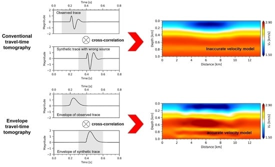
In conventional cross-correlation (CC)-based wave-equation travel-time tomography, wrong source wavelets can result in inaccurate velocity inversion results, which is known as the source–velocity trade-off. In this study, an envelope travel-time objective function is developed for wave-equation tomography to alleviate the non-uniqueness and uncertainty due to wrong source wavelets. The envelope of a seismic signal helps reduce the waveform fluctuations/distortions caused by variations of the source time function. We show that for two seismic signals generated with different source wavelets, the travel-time shift calculated by cross-correlation of their envelopes is more accurate compared to that obtained by directly cross-correlating their waveforms. Then, the CC-based envelope travel-time (ET) objective function is introduced for wave-equation tomography. A new adjoint source has also been derived to calculate the sensitivity kernels. In the numerical inversion experiments, a synthetic example with cross-well survey is first given to show that compared to the traditional CC travel-time objective function, the ET objective function is relatively insensitive to source wavelet variations and can reconstruct the elastic velocity structures more reliably. Finally, the effectiveness and advantages of our method are verified by inversion of early arrivals in a practical seismic survey for recovering near-surface velocity structures.

1. Introduction

In global- and exploration-scale seismology, compared to ray-tracing tomography methods, wave-equation-based approaches show stronger capability to recover subsurface velocity heterogeneities with higher accuracy and spatial-resolution [1,2,3,4,5,6,7,8,9]. Due to the lack of low frequencies in seismic recordings and poor initial models, the standard waveform-difference objective function in wave-equation tomography or full-waveform inversion (FWI) is prone to cycle-skipping [10,11,12,13,14,15]. Because travel-time is linearly related to the velocity perturbations, cross-correlation (CC)-based wave-equation travel-time tomography is widely used to reconstruct low-wavenumber components of the velocity models [16,17,18,19,20,21,22]. High-wavenumber model details can then be obtained using FWI with the waveform-difference objective function based on the macro background structures provided by wave-equation travel-time tomography.

In most practical applications of wave-equation based imaging/inversion methods, the source signatures (e.g., source time function, mechanism, and location) are unknown. In wave-equation travel-time tomography, if the source wavelet used in forward modeling is not accurate, the travel-time shifts calculated by cross-correlating the synthetic and observed seismic signals are also erroneous, producing unexpected uncertainties in the inverted velocity models. This issue is referred to as the source–velocity (or structure) trade-off, which has bothered geophysicists in seismic tomography for decades [23,24,25,26,27,28]. Fichtner [24] quantified source–structure trade-offs in ambient noise tomography with off-diagonal Hessian elements and mentioned that the inherent trade-offs may lead to mispositioning of structural heterogeneities. Joint inversion of the source wavelet and velocity structures represents one potential strategy to overcome this problem. However, simultaneous inversion of model parameters with different dimensionalities also suffers from the problem of interparameter trade-off [29,30,31], leading to inaccurate velocity and source inversion results. Truncated-Newton (or Gauss–Newton) optimization methods are promising to reduce these trade-off uncertainties by applying the inverse Hessian implicitly [32,33]. However, calculating Hessian-vector products in linear conjugate-gradient methods increases the algorithm complexities and computation cost significantly [32,33,34]. Yuan et al., [26] developed a double-difference objective function for wave-equation travel-time tomography with differential travel-time measurements, which can obtain higher resolution velocity structures independent of the source wavelet. However, within this approach, as the number of sources and receivers increases, the computation burden increases significantly.

The envelope measures the instantaneous amplitude of a seismic signal [35]. Wu et al., [11] recognized that the envelope fluctuation and decay of the seismic records carries ultra-low frequencies that are essentially valuable for recovering long-wavelength model structures. In FWI studies and practices, the objective functions minimizing envelope differences of synthetic and observed seismograms are widely used to suppress non-linearity of the inverse problem [11,12,13,36,37,38]. Pan and Innanen [39] revealed that the envelope-based objective functions help resolve the attenuation structures more stably. In this research, we find that envelope of the seismic signal can reduce the effects of waveform fluctuations/distortions caused by source wavelet changes. The travel-time shifts calculated by cross-correlating the seismic envelopes are relatively insensitive to wavelet errors. Thus, a CC-based envelope travel-time (ET) objective function is developed for wave-equation tomography. Derivation of the corresponding new adjoint source for calculating the velocity sensitivity kernels is provided. This ET objective function is expected to construct the velocity structures more reliably, suffering from fewer trade-off uncertainties due to inaccurate source wavelets. Compared to the Newton-based optimization methods and double-difference adjoint tomography approach, this method can be implemented more easily without increasing the computational requirements. Furthermore, this approach inherits the advantage of the envelope-difference objective function for mitigating cycle-skipping. Using the cross-correlation-based ET objective function for reducing source–velocity trade-offs has not been investigated by other researchers and represents the innovative contribution of this study.

In the numerical section, we first provide a synthetic example of elastic wave-equation travel-time tomography with a cross-well survey. Inversion experiments using the conventional CC and ET objective functions with correct- and wrong source wavelets are performed for comparison. The output results indicate that when wrong source wavelet is used in traditional CC-based wave-equation travel-time tomography, the inverted P-wave velocity $V_P$ and S-wave velocity $V_S$ perturbations are blurred with inaccurate values. However, when using the ET objective function, the elastic velocity perturbations can be recovered accurately with both correct and wrong source wavelets. This suggests that this method is less sensitive to errors of source wavelets and can reduce the trade-off uncertainties. Synthetic inversion experiments are also given to show that with large velocity contrasts, the ET objective function still works effectively. To examine the performances of the ET objective function further, we apply it to practical seismic data acquired from southeast Poland. Early arrivals are extracted from the recordings for imaging the near-surface $V_P$ model variations. It is observed that the ET objective function can resolve more detailed velocity structures with inaccurate source wavelets, suggesting that this approach works effectively and stably for noisy field data.

In this paper, the ET objective function is first introduced and the corresponding adjoint source is derived following the chain rule. The theory of conventional CC-based wave-equation travel-time tomography is given in Appendix A. Then, both synthetic inversion experiments and practical field data application are provided to verify the effectiveness and advantages of the presented method.

2. Methods

Envelope Travel-Time Wave-Equation Tomography

In wave-equation-based tomography/inversion methods, the standard objective function measures the direct waveform differences between the synthetic data $u_i$ and seismic observation $d_i$. Because the relationship between model perturbations and waveform differences is highly non-linear, this waveform-difference objective function is easily trapped at the local minimum, referring to as the cycle-skipping problem. Thus, the cross-correlation-based travel-time objective function was developed for reducing the non-linearity of wave-equation tomography [16]. The theory of conventional wave-equation travel-time tomography is introduced in Appendix A. However, when the source wavelet is inaccurate, the inverted velocity structures suffer from source–velocity trade-offs. In this section, we introduce an envelope travel-time wave-equation tomography approach for reducing the influences of wrong source wavelets.

An analytic signal ${\mathfrak{s}}_i$ can be constructed from a real signal $s_i$ and its Hilbert transform:

$${\mathfrak{s}}_i\left(t\right)=s_i\left(t\right)-\mathrm{i}\mathcal{H}\left[s_i\left(t\right)\right],$$

(1)

where i denotes the imaginary unit and $\mathcal{H}\left[s_i\left(t\right)\right]$ means Hilbert transform of $s_i$:

$$\mathcal{H}\left[s_i\left(t\right)\right]=\frac{1}{\pi }{\int }_{-\infty }^{+\infty }\frac{s_i\left(\tau \right)}{t-\tau }d\tau .$$

(2)

The analytic signal can be written in terms of instantaneous amplitude $E_i$ and instantaneous phase ${\phi }_i$:

$${\mathfrak{s}}_i\left(t\right)=E_i\left(t\right)\mathbf{exp}\left[\mathrm{i}{\phi }_i\left(t\right)\right],$$

(3)

where $E_i=\sqrt{\mathcal{R}{\left[{\mathfrak{s}}_i\left(t\right)\right]}^2+\mathcal{I}{\left[{\mathfrak{s}}_i\left(t\right)\right]}^2}$ ($\mathcal{R}$ and $\mathcal{I}$ mean real and imaginary parts) represents the envelope of the analytic signal. In FWI studies and applications, the envelope-difference objective function is commonly used to reduce the cycle-skipping problem. In this research, we reveal that the envelope of the seismic signal can reduce the fluctuations/distortions of waveforms caused by inaccurate source wavelets.

Figure 1 shows a minimum phase wavelet $s_i$ with a dominant frequency of 10 Hz (solid-red line) and a wrong source wavelet $s_i^w$ (solid-black line). The wrong source wavelet is generated by applying phase and amplitude variations to the correct minimum phase wavelet combining with another different wavelet. The dash-dotted-red and dash-dotted-black lines indicate their envelopes ($s_{i,env}$ and $s_{i,env}^w$), respectively. $\Delta s_i$ (solid-blue line) is the difference between these two wavelets. It can be seen that the waveforms of the two wavelets are obviously different. However, their envelopes can reduce the phase and amplitude distortions. We generate observed trace $d_i$ and synthetic trace $u_i^c$ using the same minimum phase wavelet, as shown in Figure 2a,b. $d_{i,env}$ and $u_{i,env}^c$ are their envelopes, respectively. Travel-time difference between the observed and synthetic traces is exactly 0.2 s. In Figure 2c, the synthetic trace $u_i^w$ with the wrong wavelet and its envelope $u_{i,env}^w$ are plotted. Then, we calculate the cross-correlation $c_i$ between $d_i$ and $u_i^c$, as plotted in Figure 2d. An exact travel-time shift 0.2 s can be obtained. $c_i^w=d_i\otimes u_i^w$ means the cross-correlation between the observed trace and the synthetic trace with the wrong wavelet (⊗ means cross-correlation). The travel-time shift is obtained as 0.187 s with 6.5% error. $c_{i,env}^w=d_{i,env}\otimes u_{i,env}^w$ is the cross-correlation between the observed trace envelope and the synthetic trace envelope with the wrong wavelet. The obtained travel-time shift is 0.2004 s with 0.2% error. This means that when the source wavelet is wrong, cross-correlation of the envelopes can produce a more accurate travel-time shift.

Thus, in this study, we introduce the ET objective function for wave-equation tomography to mitigate the influence of inaccurate source wavelets in velocity inversion:

$${\varphi }_{et}\left(\mathbf{m}\right)=\frac{1}{2}\sum _i{\left[\Delta t_i^{et}\right]}^2,$$

(4)

where the travel-time difference $\Delta t_i^{et}$ is obtained by correlating the envelopes of synthetic and observed seismic traces:

$$\Delta t_i^{et}=\underset{\tau }{argmax}{\int }_0^T{E}_i\left(t+\tau \right)E_i^{obs}\left(t\right)dt,$$

(5)

where $E_i$ and $E_i^{obs}$ are the envelopes of synthetic and observed seismic data. Variation of the ET objective function with respect to the model perturbation is given by:

$$\Delta {\varphi }_{et}=-\Delta t_i^{et}\Delta \Delta t_i^{et},$$

(6)

where $\Delta \Delta t_i^{et}$ means the variation of travel-time shift corresponding to model perturbation:

$$\Delta \Delta t_i^{et}=\frac{1}{N_{et}}\left[{\partial }_t{E}_i\left(t\right)\right]\Delta E_i\left(t\right),$$

(7)

where $N_{et}$ in the denominator is:

$$N_{et}={\int }_0^T\left[{\partial }_t^2{E}_i\left(t\right)\right]E_i\left(t\right)dt,$$

(8)

and $\Delta E_i$ represents the variation of envelope:

$$\Delta E_i\left(t\right)=\frac{u_i\left(t\right)\Delta u_i\left(t\right)+\mathcal{H}\left[u_i\left(t\right)\right]\Delta \mathcal{H}\left[u_i\left(t\right)\right]}{E_i\left(t\right)}.$$

(9)

Substituting Equation (9) into Equation (7) gives [40]:

$$\Delta \Delta t_i^{et}=\frac{\left[{\partial }_t{E}_i\left(t\right)\right]u_i\left(t\right)}{N_{et}{E}_i\left(t\right)}\Delta u_i\left(t\right)-\mathcal{H}\left\{\frac{\left[{\partial }_t{E}_i\left(t\right)\right]\mathcal{H}\left[u_i\left(t\right)\right]}{N_{et}{E}_i\left(t\right)}\right\}\Delta u_i\left(t\right).$$

(10)

Inserting Equation (10) into Equation (6), we obtain

$$\Delta {\varphi }_{et}=-\Delta t_i^{et}\frac{\left[{\partial }_t{E}_i\left(t\right)\right]u_i\left(t\right)}{N_{et}{E}_i\left(t\right)}\Delta u_i\left(t\right)+\Delta t_i^{et}\mathcal{H}\left\{\frac{\left[{\partial }_t{E}_i\left(t\right)\right]\mathcal{H}\left[u_i\left(t\right)\right]}{N_{et}{E}_i\left(t\right)}\right\}\Delta u_i\left(t\right).$$

(11)

Thus, we can derive the adjoint source of the ET objective function for calculating the velocity sensitivity kernels as:

$$s_{i,et}^{*}\left(t\right)=-\Delta t_i^{et}{P}_i\left(T-t\right)u_i\left(T-t\right)+\Delta t_i^{et}\mathcal{H}\left\{P_i\left(T-t\right)\mathcal{H}\left[u_i\left(T-t\right)\right]\right\},$$

(12)

where $P_i$ is

$$P_i\left(t\right)=\frac{{\partial }_t{E}_i\left(t\right)}{N_{et}{E}_i\left(t\right)}.$$

(13)

This ET objective function can be implemented easily and is expected to recover the velocity structures more accurately by reducing the trade-off uncertainties caused by wrong source wavelets.

3. Numerical Results

In this section, we present synthetic inversion experiments and field data application to verify the advantages of ET objective function for recovering velocity structures when an inaccurate source wavelet is used in forward simulations and adjoint tomography. We carry out the inversion experiments using the software package SeisElastic2D [41].

3.1. Synthetic Inversion Example with Cross-Well Survey

In the first numerical example, we design synthetic elastic velocity models with cross-well survey. Figure 3a,b show the target $V_P$ and $V_S$ velocity models with $V_P/V_S=2$. Velocity anomalies at the center parts of the target models are generated with ±10% perturbations of the background values. The initial models are homogeneous without the velocity perturbations at the center parts ($V_P=2V_S=3500$ m/s). The density model is homogeneous with $\rho =$ 1900 kg/m${}^3$. Because there is no density contrast in the elastic models, boundaries of the inversion results are not affected. A number of 14 sources and 180 receivers are arranged regularly on the left and right sides of the model, as shown in Figure 3a. The observed data are generated using the spectral-element forward modeling method with a minimum phase wavelet of 50 Hz dominant frequency, as indicated by the red line in Figure 3c. Another wrong source wavelet is also created by applying phase and amplitude variations to the correct minimum phase wavelet (black line in Figure 3c).

When applying the inversion, P- and S-waves are separated in the shot profiles to invert for $V_P$ and $V_S$ models, respectively. In Figure 4a,b, we plot the discrete traces of P- and S-waves extracted from the observed data (vertical component), synthetic data with the wrong source wavelet, and their envelopes for comparison. Envelopes of the seismic traces can cancel the effects of phase variations and reduce the waveform distortions effectively. In Figure 5, the absolute travel-time shifts calculated by cross-correlating the seismic traces and their envelopes are provided for comparison. It can be seen that when using wrong source wavelet, the travel-time shifts obtained from cross-correlating envelopes are closer to those obtained with the correct source wavelet, which means that the ET objective function is more robust for calculating the travel-time shifts.

Figure 6 presents the inverted $V_P$ model perturbations using traditional CC and ET objective functions with the correct and wrong source wavelets, respectively. In Figure 7, the inverted $V_S$ model perturbations by different objective functions and source wavelets are given for comparison. It can be seen that when using the wrong source wavelet, the inverted $\Delta V_P^{cc,w}$ and $\Delta V_S^{cc,w}$ structures (Figure 6b and Figure 7b) from the traditional CC objective function are blurred. The velocity anomalies are not clearly resolved. This observation is consistent with that presented in Yuan et al., [26]. However, when using the ET objective function, the inverted $\Delta V_P^{et,w}$ and $\Delta V_S^{et,w}$ model perturbations (Figure 6d and Figure 7d) with the wrong source wavelet are comparable to those obtained with the correct wavelet. Figure 8 shows the reductions of normalized travel-time data misfits when using different objective functions and source wavelets. With the wrong source wavelet, the inversion with the traditional CC objective function stops after fewer iterations, with smaller reductions of travel-time data misfits. These observations suggest that compared to the traditional CC objective function, this ET objective function algorithm is less sensitive to source wavelet errors and thus can produce more accurate velocity estimations.

To examine the effectiveness and robustness of the ET objective function for recovering velocity structures with large contrasts, we increase the velocity perturbations at the center parts of the models from ±10% of background values to ±30%. In this condition, the inverse problem becomes more non-linear. The inversion experiments are then performed using the ET objective function with the wrong source wavelet. The reconstructed model perturbations of P- and S-wave velocities are presented in Figure 9a,b. It can be seen that the elastic velocity anomalies can still be reliably inverted. This experiment suggests that the ET objective function can work effectively for large velocity contrasts with wrong source wavelets by reducing cycle-skipping and source–velocity trade-offs.

3.2. Field Data Application

To illustrate the effectiveness and stability of the ET objective function for practical seismic data, in this section, we apply wave-equation travel-time tomography with different source wavelets to image the near-surface velocity heterogeneities using early arrivals of the practical recordings. This dataset was acquired from Poland with Vibroseis seismic sources and is publicly available.

The initial 1D $V_P$ model is created with conventional migration velocity analysis, as shown in Figure 10. The initial $V_S$ and $\rho$ models are generated with $V_S=V_P/2.5$ and $\rho =350\times V_P^{0.25}$ (Gardner’s rule) and kept unchanged in the inversion. The model is 13.5 km wide and 1.0 km deep. We extract 27 sources with an interval of 200 m from the raw dataset for inversion. The receiver spacing is 25 m. Figure 11a shows one raw shot gather. It is observed that the raw shot is contaminated by strong surface waves, but contains clear early arrivals, which are valuable for recovering near-surface $V_P$ structures. The shot gathers are pre-processed to obtain the early arrivals with a series of operations including de-noising, band-pass filtering ([10 Hz, 20 Hz]), amplitude normalization, etc., as presented in Figure 11b. Because the Vibroseis source (8–95 Hz linear sweep over 15 s) was used to generate the field data, the zero-phase Klauder source wavelet $s_i^k$ can be directly generated, as indicated by the red line in Figure 12. To examine the performance of the traditional CC and the ET objective functions, we create another wrong source wavelet $s_i^w$ by applying phase and amplitude variations to the Klauder wavelet for inversion, as indicated by the black line in Figure 12.

We first perform inversion experiments using the traditional CC objective function with the correct Klauder wavelet and wrong source wavelet. The inversion results ($V_P^{cc,k}$ and $V_P^{cc,w}$) are plotted in Figure 13a,b for comparison. The corresponding model perturbations ($\Delta V_P^{cc,k}$ and $\Delta V_P^{cc,w}$) are presented in Figure 14a,b, respectively. Data misfits reduction histories are plotted in Figure 15. It can be seen that when using the correct Klauder wavelet, detailed velocity structures at the near-surface (0.0–1.0 km) can be resolved. A low-velocity zone at shallow parts (approximately 0–0.2 km) and a high-velocity formation at depths of approximately 0.3–0.7 km can be imaged clearly. Due to the limitation of source illumination, only the velocity structures at horizontal distance of 2.0–10.0 km are recovered. However, when using the wrong source wavelet, the inversion stops with fewer iterations, as indicated by the dash-dotted-black line in Figure 15. Only the low-velocity zone at shallow depth is recovered. The whole velocity model is blurred and inaccurate. Then, we carry out inversion experiments using the ET objective function with the correct and wrong source wavelets. Figure 13c,d show the inverted models ($V_P^{et,k}$ and $V_P^{et,w}$), respectively. Figure 14c,d present the corresponding model perturbations ($\Delta V_P^{et,k}$ and $\Delta V_P^{et,w}$). We observe that the inverted velocity structures by the ET objective function are very close to those obtained by the traditional CC objective function with the correct source (Figure 13a). Even though the wrong source wavelet is used, the ET objective function can still recover the low- and high-velocity zones clearly and reduce the travel-time shifts significantly, as indicated by the dash-dotted-red line in Figure 15. In Figure 16a, the observed traces, synthetic traces calculated using initial model and wrong source wavelet, and the synthetic traces calculated from the inverted model by the traditional CC objective function are plotted for comparison. After inversion, the travel-time shifts between the synthetic traces and observed traces are still very large. However, the envelopes of the synthetic traces calculated from the inverted model by the ET objective function match the envelopes of the observed traces closely, as indicated by the gray arrows in Figure 16b. These observations suggest that compared to the traditional CC objective function, the ET objective function is less sensitive to the variation of the source wavelet and thus can reduce source–velocity trade-offs. This field data application example also suggests that our new method can work effectively for other non-Vibroseis datasets with unknown source wavelets.

Finally, we design a synthetic inversion example to examine the credibility of the inversion results presented in Figure 13, which is equivalent to a resolution test. The target model is created by adding the velocity perturbation $\Delta V_P$ (Figure 17) to the initial $V_P$ model (Figure 10). The initial model used for inversion is the same as that (Figure 10) used in the practical data applications. Both the traditional CC and ET objective functions are used to recover the velocity perturbations with the correct Klauder wavelet and wrong source wavelet (Figure 12). The inversion parameters and settings are the same as those in the practical applications described above. The recovered model perturbations are presented in Figure 18. Compared to the traditional CC objective function, the ET objective function can recover the velocity anomalies more accurately and reliably, which is consistent with the observations in the practical data application. This test means that the inversion results in Figure 13 by different objective functions and source wavelets are convincing.

4. Discussions

In this study, we discuss and investigate the problem of source–velocity trade-offs in wave-equation travel-time tomography. This issue also exists in FWI with the waveform-difference objective function. Different source-independent algorithms have been developed for FWI [42,43,44,45]. However, these strategies may not be effective for inversion of seismic travel-time measurements and also suffer from the cycle-skipping challenge. Compared to the double-difference travel-time objective function proposed by Yuan et al., [26], our method can be implemented more easily without increasing the computation cost.

In wave-equation travel-time tomography, the inversion results are also affected by other source signatures including source mechanism and location. Here, the ET objective function only works for reducing the trade-offs caused by inaccurate source time functions. In travel-time tomography applications, P- and S-waves are always separated to invert for P- and S-wave velocities, respectively. In this condition, the influences of the source mechanism are limited. In exploration seismology, the source locations are always known. However, in earthquake seismology, the effects caused by inaccurate source locations should be carefully addressed.

In the inversion practices with traditional CC and ET objective functions, we realize that velocity perturbations also result in amplitude fluctuations of the waveforms. These effects produce errors in the calculation of travel-time shifts and estimation of velocity structures [20]. Furthermore, it is noticed that the ET objective function is more robust to these amplitude distortions. However, in some cases, the ET objective function does not work well for reducing the influences of wrong source wavelets. For examples, when the source wavelets contain many irregular slide lobes or the correct and wrong source wavelets have different frequency bands, this approach cannot produce very accurate velocity inversion results. In the large velocity contrasts example, the ET objective function inverts for the models effectively. However, if the model perturbations are increased further, the ET objective function may fail due to cycle-skipping.

5. Conclusions

In traditional cross-correlation based wave-equation travel-time tomography, the inversion results suffer from uncertainties caused by source–velocity trade-offs. In this research, we have revealed that the envelope of a seismic signal helps in reducing the amplitude and phase distortions caused by inaccurate source wavelets. The travel-time shifts calculated by cross-correlating envelopes are less sensitive to the variations of source wavelets. Thus, an envelope travel-time objective function is designed for wave-equation tomography. Derivation of the adjoint source for this envelope travel-time objective function is also provided. Compared to the traditional approach, this method is expected to recover the velocity structures more accurately with wrong source wavelets by suppressing the effects of source–velocity trade-offs. In the synthetic inversion experiments and field data applications, we verify that when a wrong source wavelet with phase and amplitude changes is used in forward modeling and tomography, the envelope travel-time objective function can still calculate the travel-time shifts accurately and invert for the velocity models reliably.

References

- Tarantola, A. Inversion of seismic reflection data in the acoustic approximation. Geophysics 1984, 49, 1259–1266. [Google Scholar] [CrossRef]
- Woodward, M. Wave-equation tomography. Geophysics 1992, 57, 231–248. [Google Scholar] [CrossRef]
- Pratt, R.G.; Shin, C.; Hicks, G.J. Gauss-Newton and full Newton methods in frequency-space seismic waveform inversion. Geophys. J. Int. 1998, 133, 341–362. [Google Scholar] [CrossRef]
- Tromp, J.; Tape, C.; Liu, Q. Seismic tomography, adjoint methods, time reversal, and banana-doughnut kernels. Geophysics 2005, 160, 195–216. [Google Scholar] [CrossRef] [Green Version]
- Xie, X.; Jin, S.; Wu, R. Wave-equation-based seismic illumination analysis. Geophysics 2006, 71, S169–S177. [Google Scholar] [CrossRef]
- Tape, C.; Liu, Q.; Maggi, A.; Tromp, J. Adjoint tomography of the southern California crust. Science 2009, 325, 988–992. [Google Scholar] [CrossRef] [PubMed] [Green Version]
- Wu, R.; Wang, B.; Hu, C. Renormalized nonlinear sensitivity kernel and inverse thin-slab propagator in T-matrix formalism for wave-equation tomography. Inverse Probl. 2015, 31, 115004. [Google Scholar] [CrossRef] [Green Version]
- Bozdağ, E.; Peter, D.; Lefebvre, M.; Komatitsch, D.; Tromp, J.; Hill, J.; Podhorszki, N.; Pugmire, D. Global adjoint tomography: First-generation model. Geophys. J. Int. 2016, 207, 1739–1766. [Google Scholar] [CrossRef] [Green Version]
- Operto, S.; Miniussi, A. On the role of density and attenuation in 3D multi-parameter visco-acoustic VTI frequency-domain FWI: An OBC case study from the North Sea. Geophys. J. Int. 2018, 213, 2037–2059. [Google Scholar] [CrossRef] [Green Version]
- Bunks, C.; Saleck, F.M.; Zaleski, S.; Chavent, G. Multiscale seismic waveform inversion. Geophysics 1995, 60, 1457–1473. [Google Scholar] [CrossRef]
- Wu, R.; Luo, J.; Wu, B. Seismic envelope inversion and modulation signal model. Geophysics 2014, 79, WA13–WA24. [Google Scholar] [CrossRef]
- Yuan, Y.O.; Simons, F.J.; Bozdaǧ, E. Multiscale adjoint waveform tomography for surface and body waves. Geophysics 2015, 80, R281–R302. [Google Scholar] [CrossRef] [Green Version]
- Luo, J.; Wu, R. Seismic envelope inversion: Reduction of local minima and noise resistance. Geophys. Prospect. 2015, 63, 597–614. [Google Scholar] [CrossRef]
- Métivier, L.; Brossier, R.; Mérigot, Q.; Oudet, E.; Virieux, J. Measuring the misfit between seismograms using an optimal transport distance: Application to full waveform inversion. Geophys. J. Int. 2016, 205, 345–377. [Google Scholar] [CrossRef]
- Yao, G.; Wu, D.; Wang, S. A review of reflection-waveform inversion. Pet. Sci. 2020, 17, 334–351. [Google Scholar] [CrossRef] [Green Version]
- Luo, Y.; Schuster, G.T. Wave-equation traveltime inversion. Geophysics 1991, 56, 645–653. [Google Scholar] [CrossRef]
- Zhou, C.; Schuster, G.T.; Hassanzadeh, S.; Harris, J.M. Elastic wave equation traveltime and waveform inversion of crosswell data. Geophysics 1997, 62, 853–868. [Google Scholar] [CrossRef]
- Leeuwen, T.; Mulder, W.A. A correlation-based misfit criterion for wave-equation traveltime tomography. Geophys. J. Int. 2010, 182, 1383–1394. [Google Scholar] [CrossRef] [Green Version]
- Chi, B.; Dong, L.; Liu, Y. Correlation-based reflection full-waveform inversion. Geophysics 2015, 80, R189–R202. [Google Scholar] [CrossRef]
- Luo, Y.; Ma, Y.; Wu, Y.; Liu, H.; Gao, L. Full-traveltime inversion. Geophysics 2016, 81, R261–R274. [Google Scholar] [CrossRef]
- Zheng, Y.; Wang, Y.; Luo, Q.; Chang, X.; Zeng, R.; Wang, B.; Zhao, X. Frequency-dependent reflection wave-equation traveltime inversion from walkaway vertical seismic profile data. Geophysics 2019, 84, R947–R961. [Google Scholar] [CrossRef]
- Feng, B.; Xu, W.; Wu, R.; Xie, X.; Wang, H. Finite-frequency traveltime tomography using the Generalized Rytov approximation. Geophys. J. Int. 2020, 221, 1412–1426. [Google Scholar] [CrossRef]
- Zhang, H.; Thurber, C.H. Double-difference tomography: The method and its application to the Hayward Fault, California. Bull. Seismol. Soc. Am. 2003, 3, 1875–1889. [Google Scholar] [CrossRef]
- Fichtner, A. Full Seismic Waveform Inversion for Structural and Source Parameters. Ph.D. Thesis, Ludwig Maximilian University, Munich, Germany, 2010. [Google Scholar]
- Fichtner, A. Source-structure trade-offs in ambient noise correlations. Geophys. J. Int. 2015, 202, 678–694. [Google Scholar] [CrossRef] [Green Version]
- Yuan, Y.O.; Simons, F.J.; Tromp, J. Double-difference adjoint seismic tomography. Geophys. J. Int. 2016, 206, 1599–1618. [Google Scholar] [CrossRef] [Green Version]
- Sager, K.; Ermert, L.; Boehm, C.; Fichtner, A. Towards full waveform ambient noise inversion. Geophys. J. Int. 2018, 212, 566–590. [Google Scholar] [CrossRef]
- Blom, N.; Hardalupas, P.S.; Rawlinson, N. Mitigating the effect of errors in source parameters on seismic (waveform) tomography. Geophys. J. Int. 2022, 232, 810–828. [Google Scholar] [CrossRef]
- Operto, S.; Gholami, Y.; Prieux, V.; Ribodetti, A.; Brossier, R.; Métivier, L.; Virieux, J. A guided tour of multiparameter full waveform inversion with multicomponent data: From theory to practice. Lead. Edge 2013, 32, 1040–1054. [Google Scholar] [CrossRef]
- Pan, W.; Innanen, K.A.; Margrave, G.F.; Fehler, M.C.; Fang, X.; Li, J. Estimation of elastic constants for HTI media using Gauss-Newton and full-Newton multiparameter full-waveform inversion. Geophysics 2016, 81, R275–R291. [Google Scholar] [CrossRef]
- Pan, W.; Geng, Y.; Innanen, K.A. Interparameter trade-off quantification and reduction in isotropic-elastic full-waveform inversion: Synthetic experiments and Hussar data set application. Geophys. J. Int. 2018, 213, 1305–1333. [Google Scholar] [CrossRef]
- Métivier, L.; Bretaudeau, F.; Brossier, R.; Virieux, J.; Operto, S. Full waveform inversion and the truncated Newton method: Quantitative imaging of complex subsurface structures. Geophys. Prospect. 2014, 62, 1353–1375. [Google Scholar] [CrossRef] [Green Version]
- Pan, W.; Innanen, K.A.; Liao, W. Accelerating Hessian-free Gauss-Newton full-waveform inversion via l-BFGS preconditioned conjugate-gradient algorithm. Geophysics 2017, 32, R49–R64. [Google Scholar] [CrossRef]
- Epanomeritakis, I.; Akçelik, V.; Ghattas, O.; Bielak, J. A Newton-CG method for large-scale three-dimensional elastic full-waveform seismic inversion. Inverse Probl. 2008, 24, 034015. [Google Scholar] [CrossRef]
- Taner, M.T.; Koehler, F.; Sheriff, R.E. Complex seismic trace analysis. Geophysics 1979, 44, 1041–1063. [Google Scholar] [CrossRef]
- Chen, G.; Wu, R.; Wang, Y.; Chen, S. Multi-scale signed envelope inversion. J. Appl. Geophys. 2018, 153, 113–126. [Google Scholar] [CrossRef]
- Gao, Z.; Pan, Z.; Gao, J.; Wu, R. Frequency controllable envelope operator and its application in multiscale full-waveform inversion. IEEE Trans. Geosci. Remote Sens. 2019, 57, 683–699. [Google Scholar] [CrossRef]
- Hu, Y.; Wu, R.; Huang, X.; Long, Y.; Xu, Y.; Han, L. Phase-amplitude-based polarized direct envelope inversion in the time-frequency domain. Geophysics 2022, 87, R245–R260. [Google Scholar] [CrossRef]
- Pan, W.; Innanen, K.A. Amplitude-based misfit functions in viscoelastic full-waveform inversion applied to walk-away vertical seismic profile data. Geophysics 2019, 84, B335–B351. [Google Scholar] [CrossRef]
- Bozdağ, E.; Trampert, J.; Tromp, J. Misfit functions for full waveform inversion based on instantaneous phase and envelope measurements. Geophys. J. Int. 2011, 185, 845–870. [Google Scholar] [CrossRef]
- Pan, W.; Innanen, K.A.; Wang, Y. SeisElastic2D: An open-source package for multiparameter full-waveform inversion in isotropic-, anisotropic- and visco-elastic media. Comput. Geosci. 2020, 145, 104586. [Google Scholar] [CrossRef]
- Kim, H.J.; Lee, K.H. Source-independent full-waveform inversion of seismic data. Geophysics 2003, 68, 2010–2015. [Google Scholar]
- Xu, K.; Greenhalgh, S.A.; Wang, M. Comparison of source-independent methods of elastic waveform inversion. Geophysics 2006, 71, R91–R100. [Google Scholar] [CrossRef]
- Alkhalifah, T.; Choi, Y. Source-independent time-domain waveform inversion using convolved wavefields: Application to the encoded multisource waveform inversion. Geophysics 2011, 76, R125–R134. [Google Scholar]
- Zhang, Q.; Zhou, H.; Li, Q.; Chen, H.; Wang, J. Robust source-independent elastic full-waveform inversion in the time domain. Geophysics 2016, 81, R29–R44. [Google Scholar] [CrossRef]
- Liu, Q.; Tromp, J. Finite-frequency kernels based on adjoint methods. Bull. Seismol. Soc. Am. 2006, 96, 2383–2397. [Google Scholar] [CrossRef] [Green Version]
- Byrd, R.H.; Lu, P.; Nocedal, J. A limited memory algorithm for bound constrained optimization. SIAM J. Sci. Comput. 1995, 16, 1190–1208. [Google Scholar] [CrossRef]
- Nocedal, J. Updating quasi-Newton matrices with limited storage. Math. Comput. 1980, 35, 773–782. [Google Scholar] [CrossRef]
- Nocedal, L.; Wright, S.J. Numerical Optimization, 2nd ed.; Springer: Cham, Switzerland, 2006; pp. 30–63. [Google Scholar]
Figure 1.
Comparison of the source wavelets and their envelopes. The solid-red and dash-dotted-red lines indicate the original minimum phase wavelet () and its envelope (). The solid-black and dash-dotted-black lines indicate the wrong source wavelet () and its envelope (), respectively. The solid-blue line indicates the difference between the correct and wrong source wavelets ().
Figure 2.
(a) Observed trace (solid-red line) and its envelope (dash-dotted-red line); (b) synthetic trace (solid-red line) with correct wavelet and its envelope (dash-dotted-red line); (c) synthetic trace with wrong wavelet (solid-black line) and its envelope (dash-dotted-black line); (d) is the cross-correlation between observed trace and the synthetic trace (solid-red line). is the cross-correlation between and (solid-black line). is the cross-correlation between and (dash-dotted-black line).
Figure 3.
(a,b) are the true and model structures; (c) The red and black lines indicate the correct and wrong source wavelets ( and ). The red stars and blue triangles in (a) indicate the locations of sources and receivers, respectively.
Figure 4.
(a) Comparison of the traces (vertical component) of observed P-waves (black lines) and synthetic P-waves with the wrong source wavelet (red lines); The yellow and blue lines indicate their envelopes, respectively. (b) Comparison of the traces (vertical component) of observed S-waves (black lines) and synthetic S-waves with the wrong source wavelet (red lines); The yellow and blue lines are their envelopes.
Figure 5.
(a,b) show the comparisons of absolute travel-time shifts for P- and S-waves, respectively. The blue lines indicate the travel-time shifts obtained by cross-correlating the observed traces with synthetic traces using the wrong source wavelet. The yellow lines indicate the travel-time shifts obtained by cross-correlating the envelopes of the observed traces with envelopes of the synthetic traces using the wrong source wavelet. The red bars indicate the travel-time shifts obtained by cross-correlating the observed traces with the synthetic traces using the correct source wavelet.
Figure 6.
(a,b) are the inverted P-wave velocity model perturbations and by the traditional CC objective function with correct and wrong source wavelets; (c,d) are the inverted model perturbations and by the ET objective function with correct and wrong source wavelets.
Figure 7.
(a,b) are the inverted S-wave velocity model perturbations and by the traditional CC objective function with correct and wrong source wavelets; (c,d) are the inverted model perturbations and by ET objective function with correct and wrong source wavelets.
Figure 8.
(a) Reductions of the normalized travel-time data misfits for inversion; (b) reductions of the normalized travel-time data misfits for inversion. The solid-black and dash-dotted-black lines indicate the traditional CC travel-time data misfits with correct and wrong source wavelets. The solid-red and dash-dotted-red lines indicate the new ET travel-time data misfits with correct and wrong source wavelets.
Figure 9.
(a,b) are the inverted perturbations of P- and S-wave velocities and b they ET objective function with wrong source wavelets when the velocity perturbations are ±30% of the background values.
Figure 10.
The initial model. The red stars and blue triangles indicate the schematic locations of sources and receivers.
Figure 11.
(a) Raw shot gather of vertical component; (b) the shot gather after pre-processing.
Figure 12.
Comparison of the zero-phase Klauder source wavelet (, red line) with band-pass filtering of [10 Hz, 20 Hz] and wrong source wavelet (, black line).
Figure 13.
(a,b) show the inverted velocity models and by the traditional CC objective function with the correct Klauder wavelet and wrong source wavelet, respectively; (c,d) are the inverted velocity models and by the ET objective function with the correct Klauder wavelet and wrong source wavelet.
Figure 14.
(a,b) show the inverted model perturbations and by the traditional CC objective function with the correct Klauder wavelet and wrong source wavelet; (c,d) are the inverted model perturbations and by the ET objective function with the correct Klauder wavelet and wrong source wavelet.
Figure 15.
Reductions of the normalized data misfits for travel-time inversion of early arrivals. The solid-black and dash-dotted-black lines indicate traditional CC objective function data misfits with correct and wrong source wavelets. The solid-red and dash-dotted-red lines indicate the ET objective function data misfits with correct and wrong source wavelets.
Figure 16.
(a) Comparison of the observed data (black lines), synthetic data calculated with the initial model and wrong source (gray lines), and synthetic data calculated from the inverted model (Figure 13b) and wrong source (red lines); (b) comparison of the envelopes of observed data (black lines), synthetic data calculated with the initial model and wrong source (gray lines), and synthetic data calculated from the inverted model (Figure 13d) and wrong source (red lines).
Figure 17.
Target velocity perturbation .
Figure 18.
(a,b) are the recovered perturbations and by the traditional CC objective function with correct and wrong source wavelets; (c,d) are the recovered perturbations and by the ET objective function with correct and wrong source wavelets.
Publisher’s Note: MDPI stays neutral with regard to jurisdictional claims in published maps and institutional affiliations. |
© 2022 by the authors. Licensee MDPI, Basel, Switzerland. This article is an open access article distributed under the terms and conditions of the Creative Commons Attribution (CC BY) license (https://creativecommons.org/licenses/by/4.0/).
Share and Cite
MDPI and ACS Style
Pan, W.; Ma, N.; Wang, Y. An Envelope Travel-Time Objective Function for Reducing Source–Velocity Trade-Offs in Wave-Equation Tomography. Remote Sens. 2022, 14, 5223. https://doi.org/10.3390/rs14205223
AMA Style
Pan W, Ma N, Wang Y. An Envelope Travel-Time Objective Function for Reducing Source–Velocity Trade-Offs in Wave-Equation Tomography. Remote Sensing. 2022; 14(20):5223. https://doi.org/10.3390/rs14205223
Chicago/Turabian StylePan, Wenyong, Ning Ma, and Yanfei Wang. 2022. "An Envelope Travel-Time Objective Function for Reducing Source–Velocity Trade-Offs in Wave-Equation Tomography" Remote Sensing 14, no. 20: 5223. https://doi.org/10.3390/rs14205223
Note that from the first issue of 2016, this journal uses article numbers instead of page numbers. See further details here.