Repeated (4D) Marine Geophysical Surveys as a Tool for Studying the Coastal Environment and Ground-Truthing Remote-Sensing Observations and Modeling

Abstract

Sandy beaches and the nearshore environment are dynamic coastal systems characterized by sediment mobilization driven by alternating stormy and mild wave conditions. However, this natural behavior of beaches can be altered by coastal defense structures. Repeated surveys carried out with autonomous surface vehicles (ASVs) may represent an interesting tool for studying nearshore dynamics and testing the effects of mitigation strategies against erosion. We present a one-year experiment involving repeated stratigraphic and morpho-bathymetric surveys of a nearshore environment prone to coastal erosion along the Emilia-Romagna coast (NE Italy), the Lido di Dante beach, carried out between October 2020 and December 2021 using an ASV. Seafloor and subseafloor “snapshots” collected at different time intervals enabled us to delineate the seasonal variability and shed light on key controlling variables, which could be used to integrate and calibrate remote-sensing observations and modeling. The results demonstrated that repeated surveys could be successfully employed for monitoring coastal areas and represent a promising tool for studying coastal dynamics on a medium/short (years/months) timescale.

1. Introduction

Coastal areas are strongly influenced by natural and anthropogenic impacts. Several factors contribute to the disappearance of beaches around the world, including sediment traps consisting of man-made dams, uncontrolled sand extraction, and the combined effects of sea level rises and land subsidence. Subsidence induced by natural and anthropogenic causes, such as sediment compaction, withdrawal from underground aquifers, and the extraction of hydrocarbons, is a main factor controlling instability in coastal areas, as suggested by integrated geophysical and remote-sensing studies (see [1] and references therein).

Knowledge regarding the physical and geological variables that control erosion and the deposition of sediments along coasts is a fundamental step towards the conservation of these important ecosystems. This involves a combination of investigative approaches, including biological, physical, and chemical oceanography, and the assessment of the local and regional geological setting. The starting point of such studies is the analysis of the sediment–water interface and its evolution over different timescales, information that can be gathered through the periodic and frequent monitoring of submerged beaches. Seismic reflection and echographic surveys represent fundamental tools. Although under special circumstances the remote-sensing mapping of coastal areas can be achieved using satellite or aerial surveys [2], conventional marine geophysical prospections are still more accurate and could provide ground-truthing for remote-sensing techniques, which are generally limited to areas with very shallow and clear waters. A combination of remote-sensing, geodetic, and conventional geophysical surveys, complemented by direct seabed sampling, could thus be an ideal approach to this problem [3,4]. However, acquiring bathymetric and seismic reflection data in shallow water is difficult, because the average depth is often below the limit of conventional echosounders and boat accessibility, and the noise due to waves and turbulence in the water column strongly affects the quality of measurements. As a result, the nearshore area, i.e., the most dynamic environment in terms of erosional and depositional processes, is often the least investigated. The increasing use of autonomous surface vehicles (ASVs) for performing geophysical surveys of coastal areas and other applications [5,6], in combination with remote-sensing techniques, would provide an interesting opportunity to collect high-resolution data in the nearshore area and test the feasibility of repeated (4D) surveys.

Here, we present a one-year-long experiment of repeated (4D) geophysical surveys at Lido di Dante (NE Italy), along the Adriatic Sea coast, carried out with innovative techniques by means of an ASV to study the bathy-morphological and stratigraphic characteristics of the submerged beach and its dynamic behavior. Since our main purpose was testing innovative approaches to the study of impacted coastal areas, the test site was selected because it was characterized by complex dynamic processes, resulting from a combination of natural and anthropic causes. The coastal tract under study was in fact markedly impacted by long-term human interventions, particularly during our surveys, which spanned different seasons. However, the interpretation of the short-term beach variability at the seasonal scale, which would have necessitated the consideration of a wide range of observational data and high-frequency processes (such as wave climate, local tides, and storm surges) was beyond our purpose.

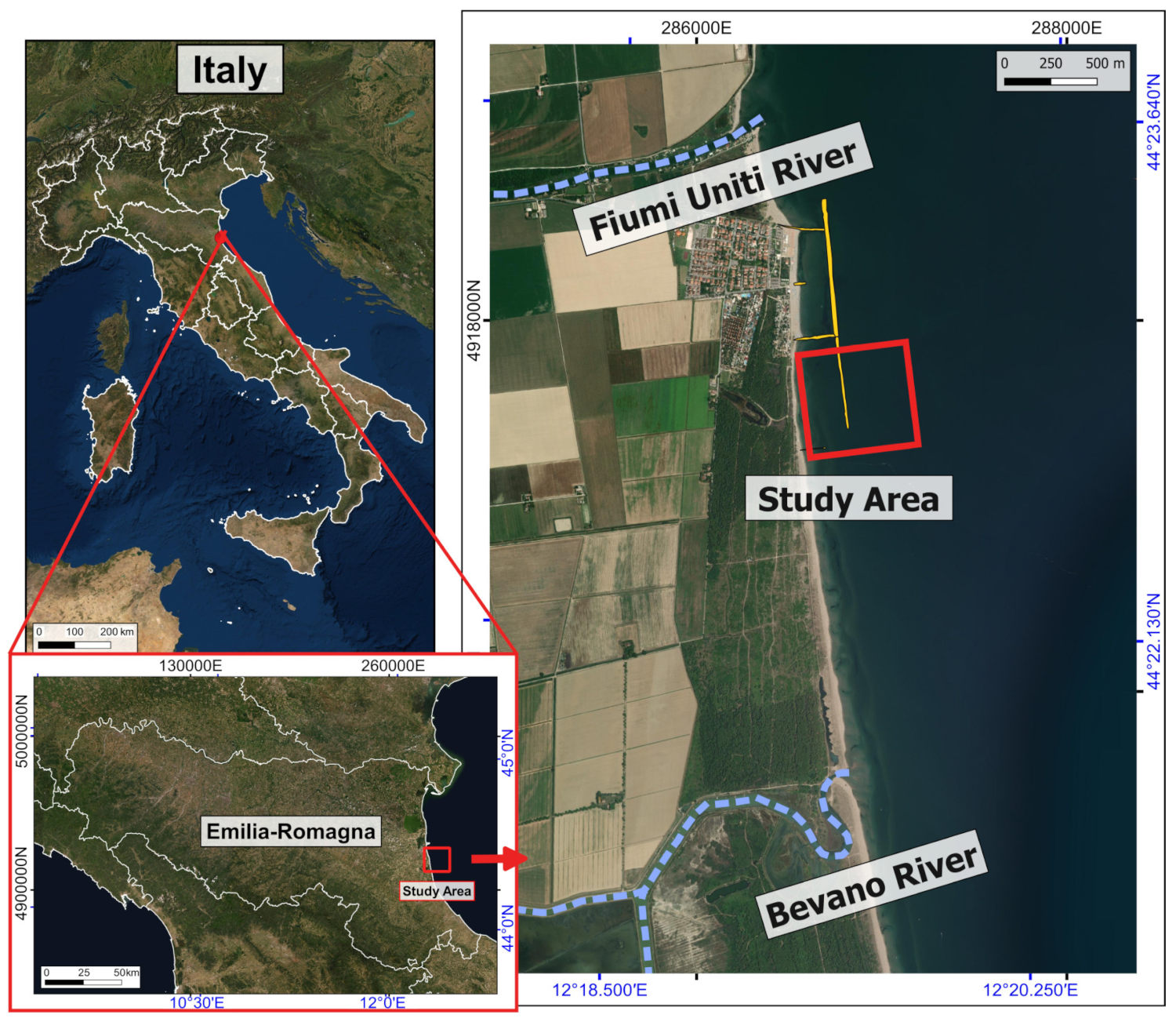
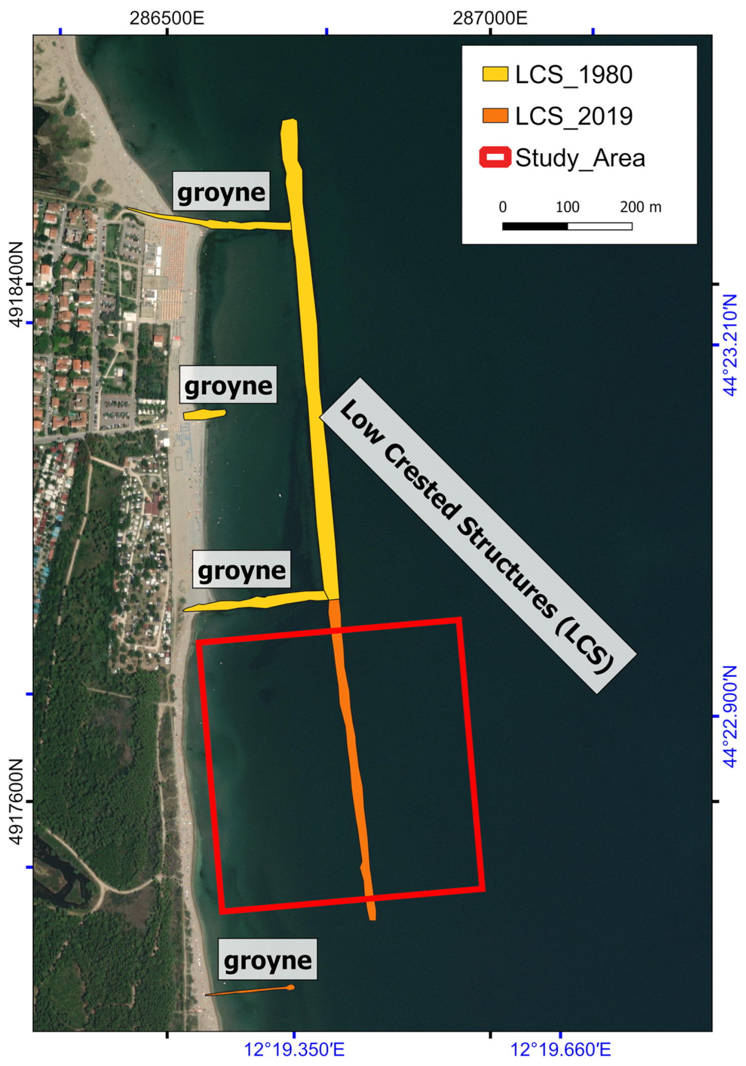
The Study Site

Lido di Dante is located in the Emilia-Romagna region coastal area, facing the Adriatic Sea in the Ravenna Municipality. This beach sector is delimited by the river mouths of the Fiumi Uniti and Bevano rivers to the north and south, respectively (Figure 1).

Despite its location, close to river outflows, Lido di Dante is affected by incipient erosion [7,8,9] due to its limited sediment supply and local subsidence enhanced by water and gas extraction [10]. Recent measurements, including high-precision leveling campaigns and GNSS measures, provided subsidence rates between 17 and 21 mm/y over the last few decades, which result higher relative to the regional average [7,8,9]. This process has led to an overall ground sinking of >50 cm in the interval 1984–2015.

Since the 1980s, part of the Lido di Dante beach has been defended by a system of shore-parallel, low-crested structures (LCSs), composed of a semi-submerged barrier and three groins (Figure 2). The almost 800 m long semi-submerged barrier is located 180 m offshore, at a water depth of 3.5 m, and was designed to emerge during low tide [11].

The southern part of the beach, extending south of the LCS system, was unprotected until recently. However, the effects of the LCSs on wave propagation were manifested just after their construction, and the localized coastal and nearshore erosion gradually propagated towards the south [7,8,9]. For this reason, in 2020 the barrier was prolonged by an additional ~500 m towards the south, and another wood groin was built (Figure 2). This sector was chosen as the study area for our tests.

Lido di Dante is a microtidal beach, with a maximum tidal range of about 0.7–1 m in the spring season [12,13]. The regional wave climate is recorded by an oceanographic buoy [7,8,9], which represents the main data source for coastal dynamic models. The most frequent conditions are characterized by wave heights reaching up to 1.0 m, directions from 90°N, and periods ranging between 5 and 7 s. Storms mostly arrive from either the NE (Bora wind) or the SE (Scirocco wind) [14]. The most energetic waves generated by Bora reach up to 4 m in height with periods of 9–11 s [14]. Scirocco storms, although commonly characterized by lower energies, are associated with a larger fetch and significant storm surges inducing a high wind set up. This wave regime is reflected by the short-term shoreline variability within the “artificially embayed” and protected Lido di Dante beach, with shoreline rotations, in either a counterclockwise or clockwise direction during Bora and Scirocco storms, respectively, as the effect of longshore currents in the opposite direction [14,15]. South of the LCSs, due to southward Bora storms, diffraction at the barrier edge generates a concentration of wave energy along the coastal stretch [16], which has experienced severe erosion in recent years [7,17]. Although the regional longshore transport direction is from south to north, a net southward longshore drift component was estimated to be ~49,000 m³/y for the submerged beach down to −7 m [16].

Presently, the Lido di Dante beach is artificially maintained through periodical nourishment. Two major interventions were carried out in 2007 and 2016, with sand volumes of about 107,100 and 122,050 m³, respectively [7,8]. It has been estimated that, to maintain the beach equilibrium, over 20,000 m³/y and 30,000–40,000 m³/y should be supplied for the area protected by the LCSs and the (previously) unprotected beach to the south, respectively [7]. Despite these nourishments, erosion is still active, and the beach is narrowing mainly in the southern stretch, where the natural dune system is subjected to overwash and overtopping during storm events [16].

A single nearshore bar with a longshore and transverse pattern was mapped in this sector before the recent prolongation of the submerged barrier [7]. In February/March 2021, a further replenishment was carried out in the nearshore area (of about 7000 m³), with the creation of an artificial bar at a depth of roughly 1.5 m that prolonged the submerged barrier by about 600 m (Figure 2). This feature acted as a “sand motor”, providing redistribution in the beach by waves and currents.

2. Materials and Methods

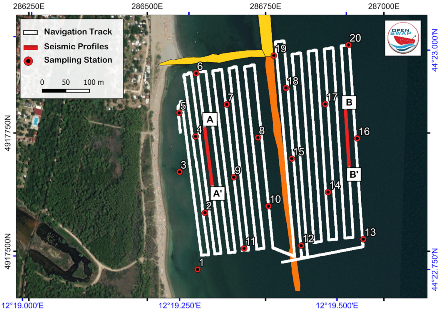
2.1. Geophysical Survey

Coastal morpho-dynamic studies require accurate estimates of beach and seafloor morphologies, as well as the analysis of their variations due to sedimentary processes. Two different strategies could be employed, involving the use of single- or multi-beam (MBES) echosounders. Although, in theory, multibeam surveys should be preferred, because the large beam width covers relatively broad sectors of the seafloor at each passage, ultra-shallow surveys carried out using single-beam echosounders present some advantages. First, the swath coverage of the MBESs decreases with depth, and in ultra-shallow waters the complexity of multibeam acquisition is not compensated for by a significant reduction in the acquisition times. Second, the increased effects of nearshore waves and turbulence approaching the coastline strongly impact the quality of MBES data, particularly those collected by lateral beams. Third, the anisotropy of the water column due to the intense mixing with air, as well as its vertical inhomogeneities caused by the fresh water supply in the nearshore area and strong temperature differences, could affect the accuracy of the beamforming procedures. All these effects could strongly limit the possibility of comparing repeated surveys. Conversely, bathymetric grids obtained by repeated passages along pre-defined tracks using single-beam echosounders enable more reliable depth and reflectivity estimates, although limited to a single profile. The possibility of comparing repeated echographic profiles or their corresponding interpolated grids as “pseudo-3D” representations of the seafloor could thus represent an interesting approach, provided that navigation lines are maintained with small errors relative to the planned routes. This latter requirement, a key factor for the feasibility of 4D (repeated) surveys, could be satisfied using an OpenSWAP ASV, which offers a maximum error within +/− 30 cm between planned and executed navigation paths in reasonable sea-state conditions [18]. Under such assumptions, and to test the potential and limits of 4D morpho-stratigraphic techniques, four repeated surveys of the study area were carried out at different times of the year, between October 2020 and December 2021 (

Table 1. List of surveys and instruments employed during the one-year experiment in the Lido di Dante study site.

Survey Number	Date	Data Collected
1	14 October 2020	- 200 kHz echosounder - Sub-bottom Chirp - Sediment sample collection
2	20 April 2021	- 200 kHz echosounder - Sub-bottom Chirp - Side-scan sonar
3	24 September 2021	- 200 kHz echosounder - Sub-bottom Chirp - Side-scan sonar
4	13 December 2021	- 200 kHz echosounder - Sub-bottom Chirp

).

2.1.1. Positioning and Navigation

During all surveys, OpenSWAP was equipped with a dual antenna differential GPS, which allowed for real-time true-heading by the autonomous navigation software. In order to obtain a homogeneous grid of bathymetric/stratigraphic data, a fixed network of planned profiles was uploaded in the navigation system of the vehicle prior to the surveys (Figure 3).

Since the main objective of our experiment was to obtain seafloor models detailed enough to be compared between relatively short time intervals (months), we first tested the accuracy of executing the planned survey lines during subsequent launches. For this purpose, a preliminary accuracy trial was performed. The results, reported in Figure 4, show that over 90% of the samples fell within 0.6 m of the expected positions, and over 50% were distributed within an error of less than 0.3 m.

2.1.2. Bathymetric Data

Bathymetric data were collected using a vertical incidence echosounder that was particularly suited to shallow-water environments, i.e., characterized by a high operating frequency (200 kHz), narrow (8° conical) beam width, short pulse length (350 µs), and a minimum depth range of ~0.3 m. Tidal oscillations were corrected using data from the tide-gauge station of Porto Corsini (12 km north of the study area), synchronized using the GNSS receiver timestamp. The 200 kHz echosounder signal was digitally sampled along a constant time window (25 ms) encompassing water column, seafloor, and sub-seafloor, and the echograms were stored in SEGY-format files. After frequency filtering and offset corrections, which were performed to account for relative offsets between the transducers and the GNSS antenna, an algorithm of bottom detection was employed to automatically identify the depth of the seabed (bottom tracking). That transit time, the so-called TWT (two-way travel), was converted into depth (m) using the average speed of sound in the water (1505 m/s, on average) measured at the beginning and end of each survey. Particular attention was devoted to filtering the effect of waves on the measures using data from the motion reference unit (MRU) onboard OpenSWAP, and in particular those relative to the vertical component. While such correction compensated for almost 90% of the wave motion, we were forced to apply a further smoothing algorithm to the bathymetric profiles to achieve a suitable correction limiting the lateral resolution of the data. In our case, this was not considered a critical problem due to the relatively high sampling rate (8 ping/s) with respect to the low speed of the vehicle during acquisition (about 2 m/s).

2.1.3. Seafloor Reflectivity

The acquisition of the entire echogram at each sounding point rather than a simple depth estimate based on an amplitude threshold gave us the opportunity to calculate seafloor reflectivity [19,20,21]. In the case of vertical incidence, neglecting the effect of energy scattering due to the bottom roughness, we could calculate the reflection coefficient (R) using:

R = (A_r/A_s) z

(1)

where A_r and A_s are the amplitudes of the source and reflected signals, respectively, and z is the water depth.

To obtain an estimate of R from our finite-length echosounder pulse, we used the following values for A_s and A_r:

$$A_s=\sum _{i=0}^W|x_i|$$

(2)

$$A_r=\sum _{i=B}^{B+W}|x_i|$$

(3)

where x(i) is the sampled signal, W is the width of the source pulse, and B is the bottom detection time. According to Equation (3), seafloor reflectivity was evaluated (together with depth) along each SEGY echographic profile using SeisPrho [22] and gridded using the nearest neighbor algorithm of the GMT software package [23] to compile reflectivity maps.

2.1.4. Stratigraphic Data

High-resolution seismic reflection profiles were acquired using a sub-bottom Chirp sonar specifically designed for OpenSWAP (µChirp [18]), integrated within the vehicle. An important feature of this system is the possibility of choosing between different emission wavelets (duration, amplitude, frequency content, etc.) depending on the target to be investigated. This allowed us to fully control the signal signature and perform reliable reflectivity estimates for seafloor and sub-seafloor targets, as well as to perform deterministic deconvolutions. Through the appropriate choice of mathematical procedures for extracting the impulse from waveforms, it is possible to achieve a remarkable improvement in the received signal resolution and amplitude.

The processing of the seismic reflection profiles was carried out using SeisPrho [22] and SEGYChange [24] and included several steps, starting from the dechirping of the frequency-modulated (FM) seismic signal through the following procedures: (i) debiasing to remove the DC component; (ii) band-pass filtering; (iii) the generation of the digital representation of the emitted FM waveform stored in the SEGY file; (iv) the cross-correlation of the digital representation of the pulse waveform with the received seismic signal; and (v) the generation of the minimum-phase wavelet and its cross-correlation with the waveform resulting from the previous steps. Further editing and processing of the seismic profiles included: swell correction, i.e., the removal of the vertical-motion wave effect (heave), and the application of a TVG (time-variant gain) compensating for spherical divergence losses.

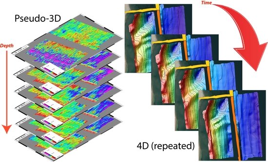
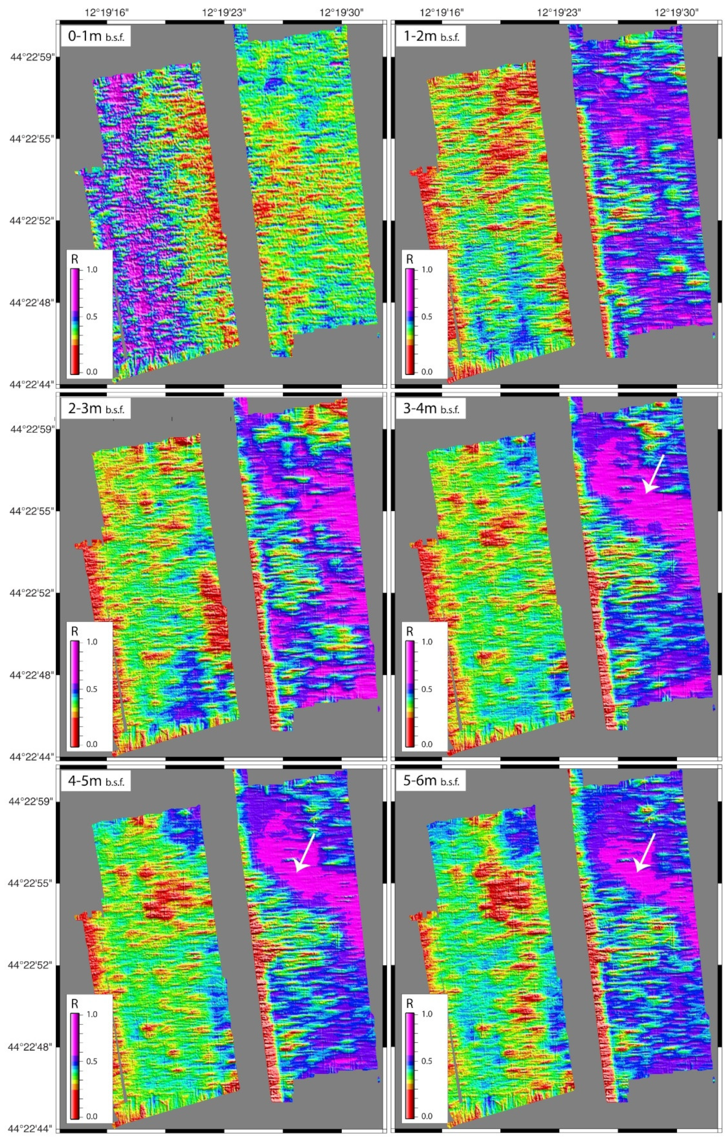
2.1.5. Flattening and Time Slicing

The densely spaced grids of the high-resolution seismic reflection profiles offered the opportunity to test pseudo-3D techniques [21] for highlighting the lateral and vertical variability of the acoustic facies. After reconstructing the amplitudes of the seismic signal by the inversion of the envelope, we removed the dipping structure from the seismic images, compiling “flattened” versions of the seismic sections using a special function of SeisPrho. These sections were obtained by time-shifting the seafloor (or any other reflector of interest within the sedimentary sequence) to form new traces in which the selected reflector was aligned at a horizontal reference level. The new set of “flattened” SEGY files was subsequently sampled at different stratigraphic levels using the Time-Slice function available in SeisPrho, which integrates seismic amplitudes (proportional to the seismic energy of reflections) within different time windows chosen based on local stratigraphy (see [21] for details). This cumulative amplitude index determined for each seismic trace was considered representative of the seismic facies and was used as a qualitative estimate of the lateral reflector’s coherence. For geological interpretation, we assumed that well-layered beddings provided higher values of this coefficient relative to chaotic deposits, a hypothesis verified in other similar cases [25,26]. In general, neatly layered seismic facies, generally corresponding to alternate levels of finer- and coarser-grained deposits, give rise to maximum values of coherence (amplitude index), while chaotic or “transparent” facies, due to, e.g., the presence of massive deposits, gas, or non-stratified layers, provide minimum amplitude indexes.

2.2. Seabed Sampling and Grain-Size Analysis

To give a geological/sedimentological ground to the echographic/seismic reflection features observed in the bathy-morphological and reflectivity maps, seafloor sediment samples were collected during the first campaign (October 2020) at twenty randomly located stations within an area of 168,000 m², at a minimum relative distance of 60 m (Figure 3 and Table S1). At each station, 50 mL of sediment was manually collected by SCUBA divers and stored at −18 °C. Grain size was determined using a Malvern Mastersizer 3000 analyzer, and laser-scattering spectra were processed using the multiple sample analysis function in the Excel worksheet GRADISTAT [27]. Grain-size analyses accounting for all particles included in the sample were reported on the GRADISTAT grain scale, modified after [28]. Based on grain-size distribution and the inflection points of cumulative curves, data were pooled into three main classes: silt and clay (<62 μm), very fine sand (62–125 μm), and fine sand and larger particles (>125 μm). Spatial analyses and the mapping of the grain-size distribution were obtained by spatial interpolation using the ordinary kriging method [29] in QGIS ver. 3.16 software [30].

Sedimentological analyses were subsequently compared to reflectivity patterns obtained by Chirp sonar data. We used the method proposed in [19], whereby the mean grain size was compared to the normalized reflectivity. This approach, though simple, was proven to be rather effective: while propagation and scattering of high-frequency acoustic signals at or near the bottom is controlled by several factors [31], experimental measurements suggest that the single most important geotechnical property related to acoustic attenuation is the mean grain size of the sediment [32,33,34,35]. The correlation between the cumulative percentage of fine sand and larger particles (>25 μm) and the reflectivity was investigated using the Pearson product-moment correlation coefficient (r), tested for difference from zero using Student’s t-distribution.

2.3. Hydrodynamic Modeling

A numerical study was implemented to simulate wave propagation and induced hydrodynamics in the study area to account for the morpho-dynamic patterns observed in the compiled maps. The coupled wave–2D hydrodynamics and sediment transport model of the Lido di Dante beach was created using the DHI suite (https://www.mikepoweredbydhi.com/ accessed date 12 January 2020). A regional 120-by-140 km digital elevation model (DEM), including our study area, was provided by ARPAe (Agenzia Regionale per l’Ambiente—Emilia-Romagna) for the purpose of the simulation (Figure 5).

The spectral waves module was based on wave heights measured by a buoy installed offshore the study site at −10 m depth in the period October 2020/April 2021. Wave-induced currents were considered alongside the 2D hydrodynamics module, based on the wave radiation stress and the sea water level (swl) measured by a tide gauge located in Porto Corsini.

3. Results

3.1. Morphobathymetry

The maps displayed in Figure 6 show the seafloor DEMs based on data collected during the four repeated surveys in the one-year experiment (Table 1).

The depth range is between 0.3 and about 4.9 m. Off the LCS, the bathymetry is dominated by a rather flat seabed regularly dipping seaward. In the inner (landward) side of the submerged barrier, the seabed is more irregular, with alternating ridges and troughs, mostly oriented ENE–WSW. These features showed some morphological differences between the surveys (Figure 6) that will be further discussed in Section 3.5. A relative minimum in the bathymetry reaching over −4 m was observed during all surveys at the southern roundhead LCS. This feature was also detected by previous bathymetric surveys [36] and was interpreted as being related to the local hydrodynamic conditions at the edges of the barrier, which caused localized seabed erosion.

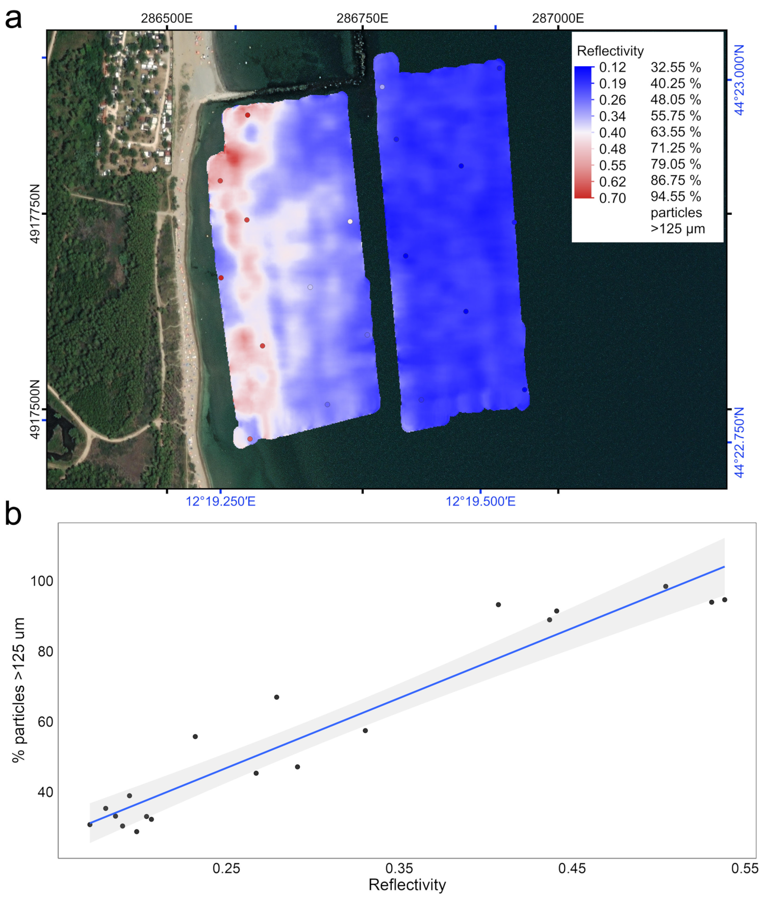
3.2. Sediment Grain Size and Reflectivity

Based on Folk and Ward’s [37] classification, seafloor sediments in the study area mostly ranged from coarse to very fine sand. The particle size distribution curve showed an inflection point corresponding to very fine sand (62–125 μm), which thus appeared to be the most distinctive class, ranging from 0.4 to 49.7% (Table S1 and Figure S1). The grain-size distribution map showed the prevalence of fine sand and larger particles close to the coastline, with an increasing seaward gradient of very fine sand, as well as a slight enrichment (commonly within a few percent) of silt and clay at the inner base of the LCSs (Figure 7).

The grain-size distribution was compared with the reflectivity map from the same campaign (Figure 8). The linear correlation between the cumulative percentage of fine sand and larger particles (>125 μm) and the normalized reflectivity showed a good fit (Figure 8b), with a correlation coefficient as high as 0.96 (p < 0.0001, n = 19).

The map in Figure 8a shows a similar pattern to that of Figure 7. This enabled us to consider the reflectivity maps obtained during the different seasonal surveys (Figure 9) as representative of grain-size distribution, even in absence of the direct sampling and analysis of the seafloor sediments.

The reflectivity maps displayed in Figure 9, collected during the four seasonal campaigns, show interesting features and significant differences, both in the normalized reflectivity values and the distribution patterns, indicating dynamics not immediately perceived in the bathymetric models alone (Figure 6). The reflectivity map of April 2021 (Figure 6b) shows an important difference compared to the other maps, with the R coefficient ranging from ≤0.2 near the LCS to a maximum of >0.9 in the nearshore area. This might suggest a discrepancy with the October 2020 pattern, probably due to the redistribution of relatively coarse-grained sediment after the 2021 nourishment intervention. It also accounts for the higher-than-expected R values off the LCSs detected in April 2021, probably indicating that part of the supplied sandy sediment passed above the semi-submerged barrier and was transported towards the offshore and along the coast.

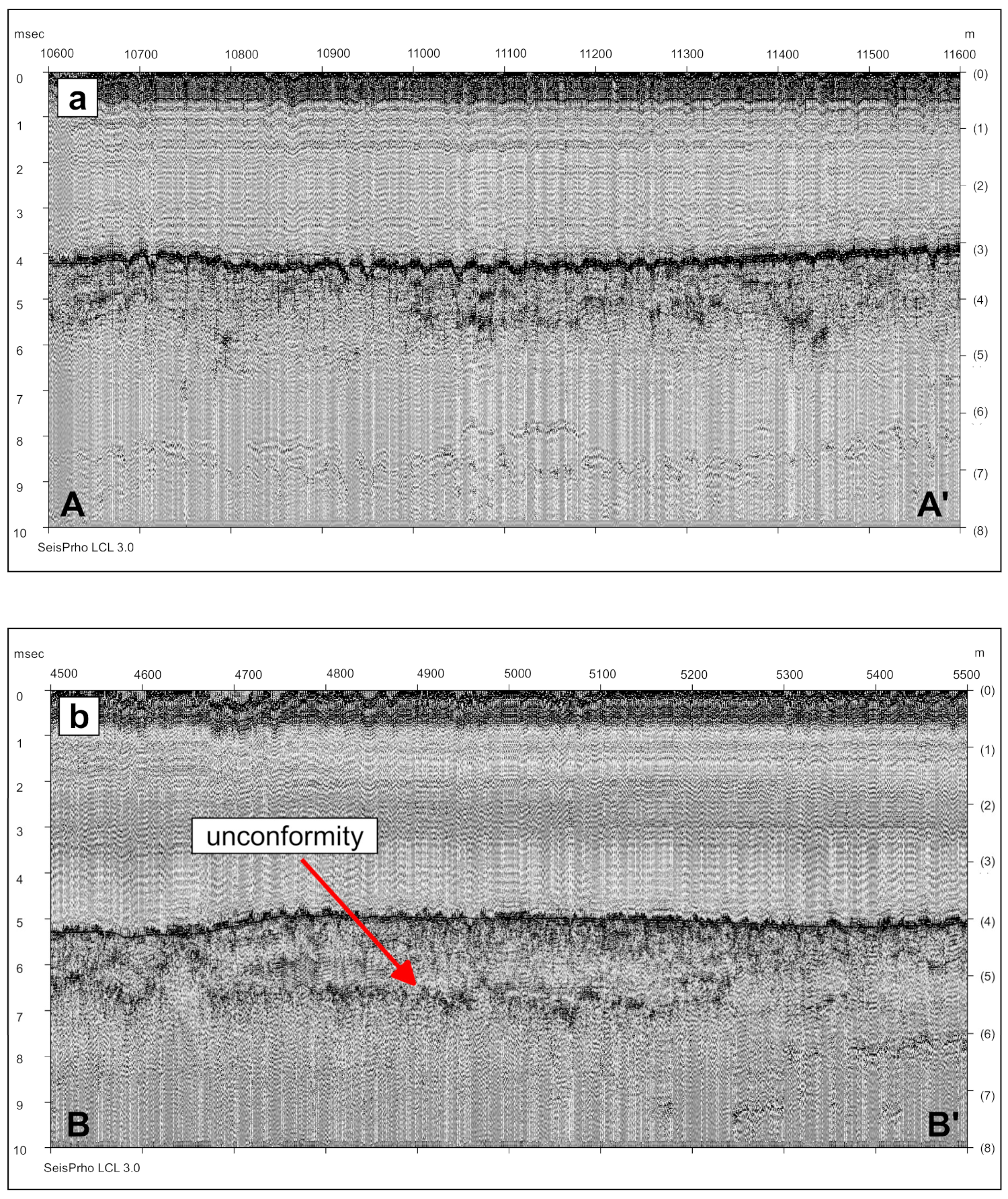
3.3. Stratigraphy

Figure 10 displays two seismic reflection profiles representative of the seismostratigraphic characteristics of the study area. We note that signal penetration into the nearshore sediments was limited to a few meters, probably due to the sandy nature of the deposits caused by the relatively high energy of the depositional processes involved.

Such features resulted in the presence, approaching the shoreline, of “massive” acoustic facies with sporadic irregular discontinuities (reflectors), probably due to lithologic vertical/lateral changes and/or to diagenetic or lithified surfaces (Figure 10a). Offshore, beyond the LCS barrier, the seismic signal penetrated deeper, showing sub-horizontal stratification up to a few meters of depth and major nonconformity (of undetermined age) ranging from 1.5 to 3.0 m below the seafloor (Figure 11).

While snapshots of the bathymetric and reflectivity changes at the seafloor could provide information about the active sedimentary processes shaping the coastal environment, the available seismic reflection profiles, penetrating the first few meters of the sedimentary sequence, could help shed light on its geological evolution. Figure 11 presents reflectivity layers extracted at different depths, each integrating (averaging) values of seismic amplitudes between one level and the next. As seen in other studies [21,26], such a technique is able to detect buried features in a way similar to that of CT-scan medical imaging techniques. In this case, we noted that below the first meter of depth reflectivity, the values increased from the coast towards the offshore area. In particular, the elongated pattern of high reflectivity (white arrow in Figure 11) ~3 m below the seafloor suggested the presence of an erosional channel filled with coarse deposits running oblique to the coastline. This feature, possibly connected in the past to the onshore river network, did not show any morphological correspondence with the present-day seafloor morphology, being covered by more recent, differently structured deposits.

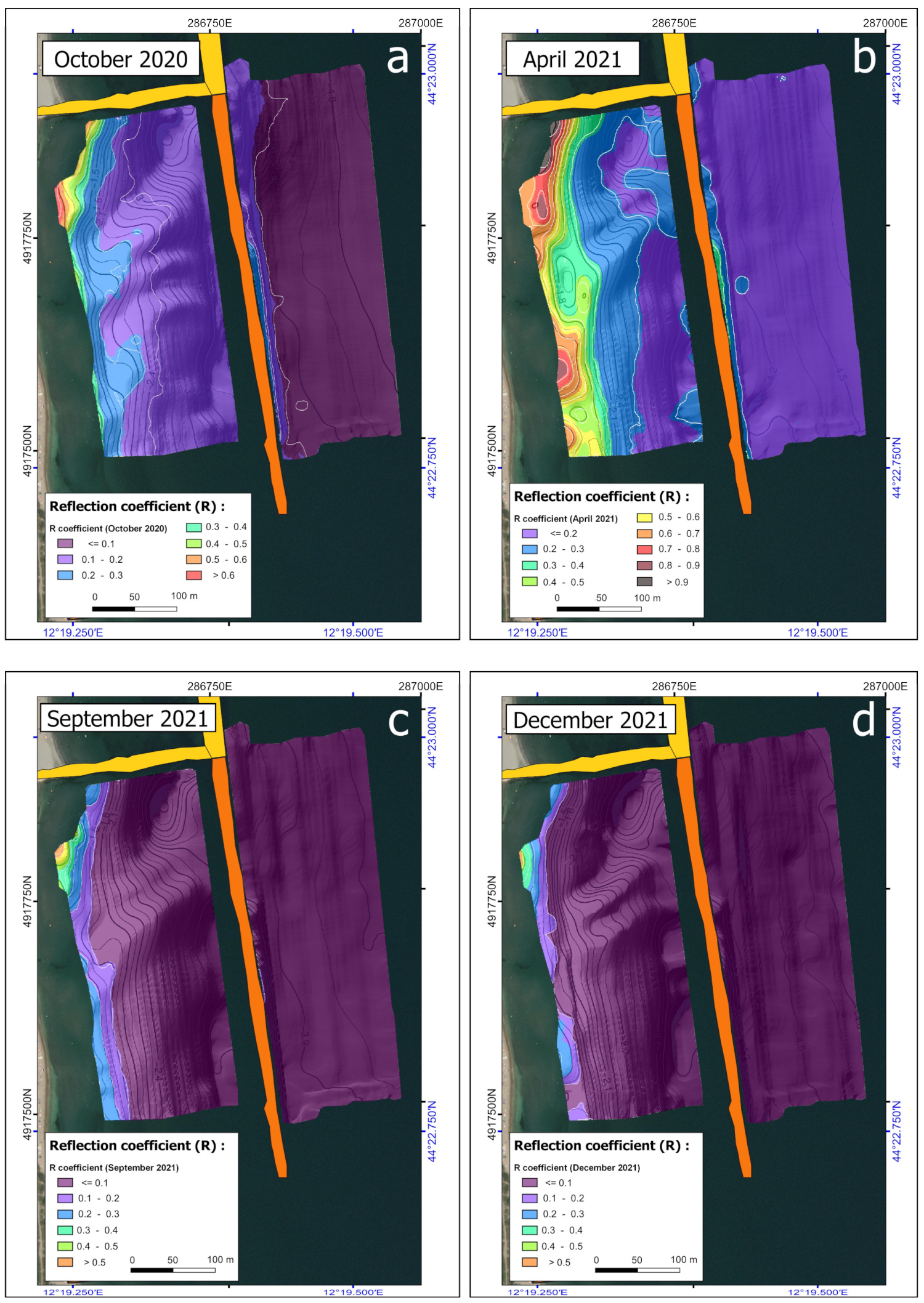
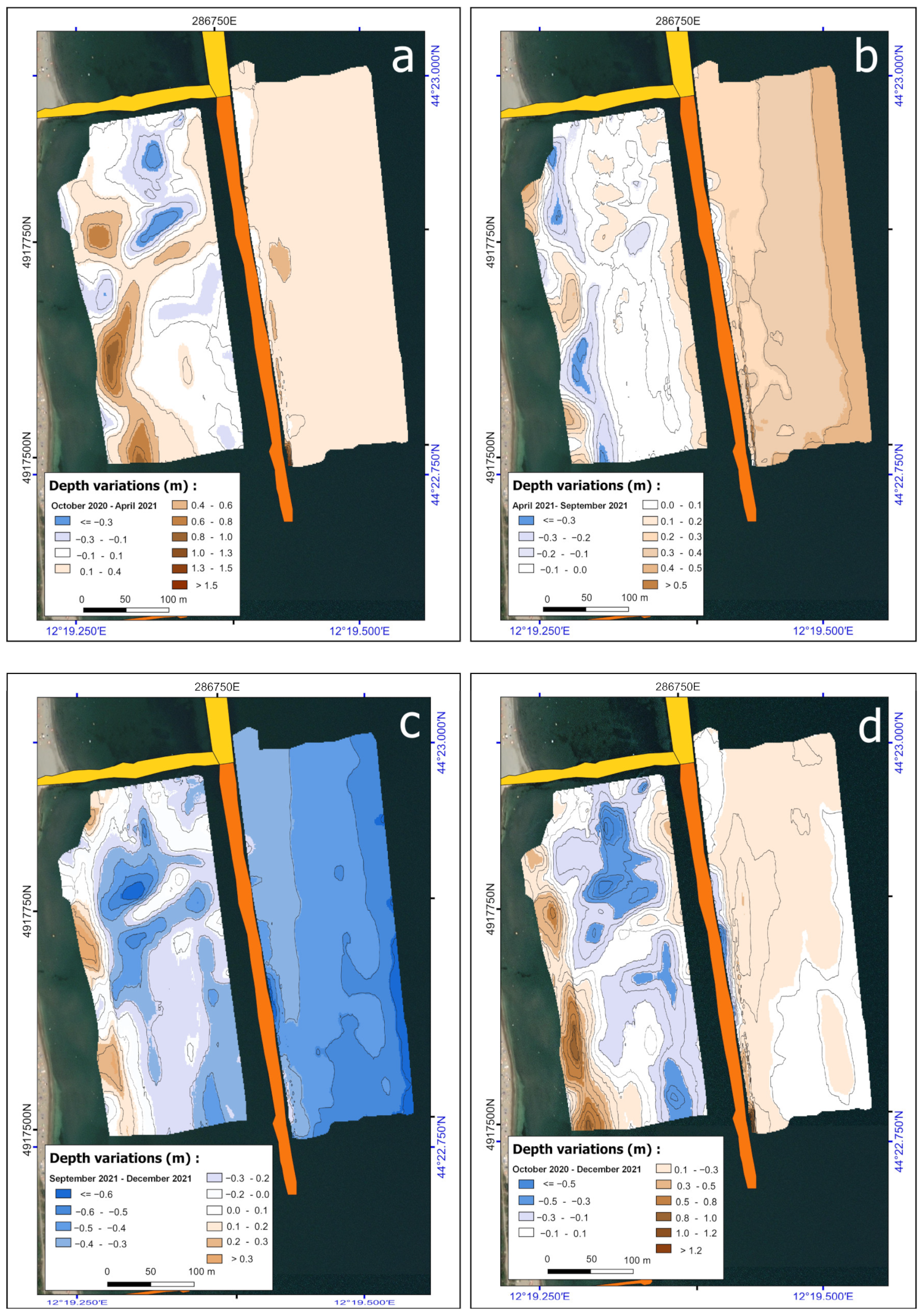
3.4. Bathy-Morphological Snapshots

To analyze the morphological changes of the seafloor and sediment transport within the study area during the one-year experiment, we compared the seafloor digital models from all surveys (Figure 12). To obtain a quantitative estimate of seafloor changes, we analyzed differential DTMs from subsequent surveys (for example, October 2020 vs. April 2021, Figure 12a). Absolute bathymetric differences were subsequently gridded and color-coded with colors ranging from light to dark brown for seabed accretion due to sediment accumulation, and from light to dark blue for sediment losses or erosion.

In Figure 12a (October 2020/April 2021), localized patches indicating accretion are visible in the nearshore area along an ENE–WSW-oriented ridge. This was likely due to the nourishment program carried out in this area in February/March 2021. A subsequent sediment redistribution, both within and beyond the LCS, also suggested by the analysis of the reflectivity patterns of Figure 9b, is shown in the April 2021/September 2021 comparison map (Figure 12b), with gradual seabed accretion up to 30–40 cm towards the offshore area on a flat seabed regularly dipping towards the sea. Conversely, in the September 2021/December 2021 differential map (Figure 12c), a flat seafloor prevailed in most of the submerged beach, probably indicating sediment redistribution/erosion that took place during the stormy winter. In the October 2020/December 2021 differential map (Figure 12d), the most evident depth variations occurred in the nearshore area, where the sediments added during the 2021 nourishment intervention were redistributed by currents, creating alternate positive and negative patterns. Very subtle seafloor changes were detected beyond the barrier, where the seafloor was characterized by a flat morphology and fine-grained sediments prevailed.

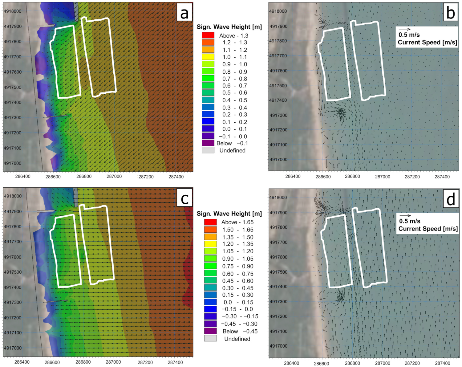
3.5. Wave Hydrodynamic Modeling

Hydrodynamic modeling in and around the study area provided us with a key to interpret the hydro- and morpho-dynamic patterns producing the observed seasonal changes. Figure 13 includes snapshots depicting the wave and current fields modeled for different conditions, such as during the storms that occurred between October 2020 and April 2021, which hit the coast from different directions. Each map displays the wave and current fields, as well as the wave boundary conditions at −10 m depth.

We observed that the heights of the waves reaching the coast were reduced by the presence of the submerged barrier. In the first case (Figure 13a,b), a storm wave with Hs = 1.63 m propagating from the NE, thus generated by Bora winds, induced a longshore current toward the S. Conversely (Figure 13c,d), waves generated by Scirocco winds during a storm from the SE produced longshore currents oriented towards the N, creating several vortexes between the coast and the submerged barriers, with sediment transport towards their lee side.

The simulation of seabed morphological changes for October 2020–April 2021 by the sediment transport module (Figure 14a) showed seabed accretion parallel to the coast, corresponding to the inner side of the submerged breakwater and other localized accretion spots in the nearshore area. Conversely, NNE–SSW-oriented nearshore erosional areas, reaching up to some tens of cm, resulted from the same model (Figure 14). The reproduced pattern of seafloor changes was similar to that observed through the bathymetric surveys presented in the October 2020/April 2021 differential map (Figure 12a and Figure 14b).

4. Discussion and Conclusions

The data collected in the study area during the one-year experiment suggested that 4D (repeated) surveys are feasible using the employed technologies, since consistent differential bathymetric and reflectivity models of the seafloor were obtained. Morphological changes, not limited to the subaerial beach but extending to the nearshore area, are more significant for evaluating the state and evolution of a coastal area than the shoreline behavior alone, which is very variable and often affected by anthropic bias [38,39]. Comparisons with independent hydrodynamic modeling also suggested an interesting fit between predicted and observed erosional/depositional patterns.

Our work suggests that these methods could be effective for monitoring coastal areas, allowing the evaluation of the key variables controlling the complex dynamics of the nearshore environment. Since they can be performed at a relatively low cost, in terms of both time and money, they could become common components of studies on coastal dynamics, the design of protection structures, and the verification of such structures’ effectiveness in limiting the progressive erosion and degradation of the natural environment. All maps compiled during this and possibly other experiments could be used as “snapshots” to capture the state of the nearshore at a certain moment and to calibrate hydrodynamic models that could predict its evolution under changing environmental variables.

The studied coastal stretch at Lido di Dante no longer represents natural conditions, and the effects of the adopted defense strategies largely control the sediment distribution and the beach’s morphological evolution. The repeated geophysical surveys show that the most active morpho-dynamic processes are confined to a very narrow sector between the coast and the submerged barriers. Here, the sediment is remobilized by waves and longshore currents that are particularly effective during storms, arriving from either the south or the north. The seabed in this most dynamic sector is characterized by coarser grain sizes, i.e., coarse/medium sand to fine sand, as shown by the grain-size distribution and reflectivity maps, while the finer fractions are mostly “cleaned up” by normal sorting processes in the nearshore area, also in the presence of protecting barriers.

Our experiment also confirmed that sediment distribution at the seafloor could be mapped using indirect methods, such as reflectivity maps, provided that preliminary data calibrations are performed through local sampling. It is crucial in this respect to avoid the saturation of the echographic signal, which could hamper the discrimination of grain-size differences in the high-reflectivity sectors.

The collection of Chirp sonar data penetrating several meters below the seafloor, together with or as an alternative to higher-frequency single-beam sensors, enables the compilation of reflectivity “time-slice” maps of the sub-seafloor, which could add a long-term perspective to the geological analysis of any study site. In this case, seismostratigraphic data should be complemented by stratigraphic information, i.e., analyses and correlations of sediment cores, which were not available for our study.

Certain technical aspects are critical for executing 4D (repeated) surveys in these environments. First and most important is the ability to repeat the planned acquisition tracks with a high degree of accuracy, within a few tens of centimeters of error; this can be achieved only by using autonomous surface vehicles. Then, most attention should be devoted to static corrections in regard to several sources, including waves (the most important factors in nearshore areas), tides, and the accurate measurement of sound velocity in the water. The measurement of these parameters should be conducted. If all these effects can be further minimized, as recent improvements in low-cost but accurate positioning systems and solid-state accelerometers might suggest, the periodic monitoring of coastal areas could become an interesting tool for marine and coastal studies.

References

- Bonetti, J.; Del Bianco, F.; Schippa, L.; Polonia, A.; Stanghellini, G.; Cenni, N.; Draghetti, S.; Marabini, F.; Gasperini, L. Anatomy of Anthropically Controlled Natural Lagoons through Geophysical, Geological, and Remote Sensing Observations: The Valli Di Comacchio (NE Italy) Case Study. Remote Sens. 2022, 14, 987. [Google Scholar] [CrossRef]
- Hodúl, M.; Bird, S.; Knudby, A.; Chénier, R. Satellite derived photogrammetric bathymetry. ISPRS J. Photogramm. Remote Sens. 2018, 142, 268–277. [Google Scholar] [CrossRef]
- Van Rijn, L. Coastal erosion and control. Ocean Coast. Manag. 2011, 54, 867–887. [Google Scholar] [CrossRef]
- Bio, A.; Bastos, L.; Granja, H.; Pinho, J.; Gonçalves, J.; Henriques, R.; Madeira, S.; Magalhães, A.; Rodrigues, D. Methods for coastal monitoring and erosion risk assessment: Two Portuguese case studies. Rev. de Gestão Costeira Integr. 2015, 15, 47–63. [Google Scholar] [CrossRef] [Green Version]
- Makar, A.; Specht, C.; Specht, M.; Dąbrowski, P.; Burdziakowski, P.; Lewicka, O. Seabed Topography Changes in the Sopot Pier Zone in 2010–2018 Influenced by Tombolo Phenomenon. Sensors 2020, 20, 6061. [Google Scholar] [CrossRef]
- Carlson, D.F.; Fürsterling, A.; Vesterled, L.; Skovby, M.; Pedersen, S.S.; Melvad, C.; Rysgaard, S. An affordable and portable autonomous surface vehicle with obstacle avoidance for coastal ocean monitoring. HardwareX 2019, 5, e00059. [Google Scholar] [CrossRef]
- Quaderni di Arpa, I.; Preti, M.; De Nigris, N.; Morelli, M.; Monti, M.; Bonsignore, F.; Aguzzi, M. (Eds.) Arpa. Stato del Litorale Emiliano-Romagnolo All’anno 2007 e Piano Decennale di Gestione; Arpa Emilia Romagna: Bologna, Italy, 2009; p. 270. ISBN 88-87854-21-1. [Google Scholar]
- Aguzzi, M.; Bonsignore, F.; De Nigris, N.; Morelli, M.; Paccagnella, T.; Romagnoli, C.; Unguendoli, S.; I quaderni di Arpae. Arpae. Stato del Litorale Emiliano-Romagnolo al 2012; Erosione e interventi di difesa; Arpae Emilia-Romagna Ed.: Bologna, Italy, 2016; p. 227. ISBN 978-88-87854-41-1. [Google Scholar]
- Quaderni di Arpae, I.; Aguzzi, M.; Costantino, R.; De Nigris, N.; Morelli, M.; Romagnoli, C.; Unguendoli, S.; Vecchi, E. (Eds.) Arpae. Stato del Litorale Emiliano-Romagnolo al 2018; Erosione e interventi di difesa; Arpae Emilia Romagna: Bologna, Italy, 2020; p. 224. ISBN 978-88-87854-48-0. Available online: https://www.arpae.it/it/notizie/slem-2018.pdf (accessed on 20 February 2021).
- Teatini, P.; Ferronato, M.; Gambolati, G.; Gonella, M. Groundwater pumping and land subsidence in the Emilia-Romagna coastland, Italy: Modeling the past occurrence and the future trend. Water Resour. Res. 2006, 42, W01406. [Google Scholar] [CrossRef]
- Lamberti, A.; Zanuttigh, B. An integrated approach to beach management in Lido di Dante, Italy. Estuar. Coast. Shelf Sci. 2005, 62, 441–451. [Google Scholar] [CrossRef]
- Armaroli, C.; Ciavola, P. Dynamics of a nearshore bar system in the northern Adriatic: A video-based morphological classi-fication. Geomorphology 2011, 126, 201–216. [Google Scholar] [CrossRef]
- Archetti, R. Quantifying the Evolution of a Beach Protected by Low Crested Structures Using Video Monitoring. J. Coast. Res. 2009, 254, 884–899. [Google Scholar] [CrossRef]
- Archetti, R.; Romagnoli, C. Analysis of the effects of different storm events on shoreline dynamics of an artificially embayed beach. Earth Surf. Process. Landf. 2011, 36, 1449–1463. [Google Scholar] [CrossRef]
- Archetti, R.; Lamberti, A.; Smith, J.M. Storm-Driven Shore Changes of a Beach Protected by a Low Crested Structure. In Coastal Engineering; World Scientific: Singapore, 2009; pp. 1977–1989. [Google Scholar] [CrossRef]
- Ciavola, P.; Armaroli, C.; Chiggiato, J.; Valentini, A.; Deserti, M.; Perini, L.; Luciani, P.; Silvani, V. Impact of storms along the coastline of Emilia-Romagna: The morphological signature on the Ravenna coastline (Italy). J. Coast. Res. 2007, 540–544. Available online: http://www.jstor.org/stable/26481647 (accessed on 15 April 2021).
- Preti, M. Ripascimento Delle Spiagge con Sabbie Sottomarine in Emilia-Romagna: Monitoraggio 2001–2009; Studi costieri N.19 2011; Arpae Emilia-Romagna Ed.: Bologna, Italy, 2011; p. 2016. [Google Scholar]
- Stanghellini, G.; Del Bianco, F.; Gasperini, L. OpenSWAP, an Open Architecture, Low Cost Class of Autonomous Surface Vehicles for Geophysical Surveys in the Shallow Water Environment. Remote Sens. 2020, 12, 2575. [Google Scholar] [CrossRef]
- Gasperini, L. Extremely Shallow-water Morphobathymetric Surveys: The Valle Fattibello (Comacchio, Italy) Test Case. Mar. Geophys. Res. 2005, 26, 97–107. [Google Scholar] [CrossRef]
- Ligi, M.; Bortoluzzi, G.; Giglio, F.; Del Bianco, F.; Ferrante, V.; Gasperini, L.; Ravaioli, M. Shallow water acoustic techniques to investigate transitional environments: A case study over Boka Kotorska bay. Measurement 2018, 126, 382–391. [Google Scholar] [CrossRef]
- Gasperini, L.; Ligi, M.; Stanghellini, G. Pseudo-3D techniques for analysis and interpretation of high-resolution marine seismic reflection data. Boll. Geofis. Teor. Appl. 2021, 62, 599–614. [Google Scholar]
- Gasperini, L.; Stanghellini, G. SeisPrho: An interactive computer program for processing and interpretation of high-resolution seismic reflection profiles. Comput. Geosci. 2009, 35, 1497–1507. [Google Scholar] [CrossRef]
- Wessel, P.; Smith, W.H.F.; Scharroo, R.; Luis, J.; Wobbe, F. Generic Mapping Tools: Improved Version Released. EOS Trans. Am. Geophys. Union 2013, 94, 409–410. [Google Scholar] [CrossRef] [Green Version]
- Stanghellini, G.; Carrara, G. Segy-change: The swiss army knife for the SEG-Y files. SoftwareX 2017, 6, 42–47. [Google Scholar] [CrossRef]
- Gasperini, L.; Marzocchi, A.; Mazza, S.; Miele, R.; Meli, M.; Najjar, H.; Michetti, A.M.; Polonia, A. Morphotectonics and late Quaternary seismic stratigraphy of Lake Garda (Northern Italy). Geomorphology 2020, 371, 107427. [Google Scholar] [CrossRef]
- Gasperini, L.; Peteet, D.; Bonatti, E.; Gambini, E.; Polonia, A.; Nichols, J.; Heusser, L. Late Glacial and Holocene environmental variability, Lago Trasimeno, Italy. Quat. Int. 2021, 622, 21–35. [Google Scholar] [CrossRef]
- Blott, S.J.; Pye, K. GRADISTAT: A grain size distribution and statistics package for the analysis of unconsolidated sediments. Earth Surf. Process. Landf. 2001, 26, 1237–1248. [Google Scholar] [CrossRef]
- Friedman, G.M.; Sanders, J.E. Principles of Sedimentology; Wiley: New York, NY, USA, 1978. [Google Scholar]
- Zhang, H.; Lu, L.; Liu, Y.; Liu, W. Spatial Sampling Strategies for the Effect of Interpolation Accuracy. Int. J. Geo-Inf. 2015, 4, 2742–2768. [Google Scholar] [CrossRef]
- QGIS Development Team. QGIS Geographic Information System Version 3.16.5 LTR. 2021. Available online: http://qgis.osgeo.org (accessed on 1 March 2021).
- Richardson, M.D.; Briggs, K.B. In situ and laboratory geoacoustic measurements in soft mud and hard-packed sand sediments: Implications for high-frequency acoustic propagation and scattering. Geo-Mar. Lett. 1996, 16, 196–203. [Google Scholar] [CrossRef]
- Shumway, G. Sound Speed and Absorption Studies of Marine Sediments by a Resonance Method. Geophysics 1960, 25, 451–467. [Google Scholar] [CrossRef]
- McCann, C.; McCann, D.M. The Attenuation of Compressional Waves in Marine Sediments. Geophysics 1969, 34, 882–892. [Google Scholar] [CrossRef]
- McCann, C.; McCann, D.M. A theory of compressional wave attenuation in non-cohesive sediments. Geophysics 1985, 50, 1311–1317. [Google Scholar] [CrossRef]
- Dunlop, J.I. Measurement of acoustic attenuation in marine sediments by impedance tube. J. Acoust. Soc. Am. 1992, 91, 460–469. [Google Scholar] [CrossRef]
- Zanuttigh, P.; Brusco, N.; Taubman, D.; Cortelazzo, G. A novel framework for the interactive transmission of 3D scenes. Signal Process. Image Commun. 2006, 21, 787–811. [Google Scholar] [CrossRef]
- Folk, R.L.; Ward, W.C. Brazos river bar: A Study in the Significance of Grain-Size Parameters. J. Sediment. Res. 1957, 27, 3–26. [Google Scholar] [CrossRef]
- MATTM-Regioni. Linee Guida Nazionali per la Difesa Della Costa dai Fenomeni di Erosione e Dagli Effetti dei Cambiamenti Climatici. 2018, p. 305. Available online: http://www.erosionecostiera.isprambiente.it/files/linee-guida-nazionali/TNEC_LineeGuidaerosionecostiera_2018.pdf (accessed on 1 March 2021).
- Romagnoli, C.; Sistilli, F.; Cantelli, L.; Aguzzi, M.; De Nigris, N.; Morelli, M.; Gaeta, M.G.; Archetti, R. Beach Monitoring and Morphological Response in the Presence of Coastal Defense Strategies at Riccione (Italy). J. Mar. Sci. Eng. 2021, 9, 851. [Google Scholar] [CrossRef]