
Potential of Time-Series Sentinel 2 Data for Monitoring Avocado Crop Phenology


Applied Agricultural Remote Sensing Centre, University of New England, Armidale, NSW 2351, Australia
*
Author to whom correspondence should be addressed.
Remote Sens. 2022, 14(23), 5942; https://doi.org/10.3390/rs14235942
Submission received: 20 October 2022
/
Revised: 21 November 2022
/
Accepted: 21 November 2022
/
Published: 24 November 2022
(This article belongs to the Special Issue Crop Growth Monitoring Using Remote Sensing: Progress, Challenges and Opportunities)
Abstract
:The ability to accurately and systematically monitor avocado crop phenology offers significant benefits for the optimization of farm management activities, improvement of crop productivity, yield estimation, and evaluation crops’ resilience to extreme weather conditions and future climate change. In this study, Sentinel-2-derived enhanced vegetation indices (EVIs) from 2017 to 2021 were used to retrieve canopy reflectance information that coincided with crop phenological stages, such as flowering (F), vegetative growth (V), fruit maturity (M), and harvest (H), in commercial avocado orchards in Bundaberg, Queensland and Renmark, South Australia. Tukey’s honestly significant difference (Tukey-HSD) test after one-way analysis of variance (ANOVA) with EVI metrics (EVImean and EVIslope) showed statistically significant differences between the four phenological stages. From a Pearson correlation analysis, a distinctive seasonal trend of EVIs was observed (R = 0.68 to 0.95 for Bundaberg and R = 0.8 to 0.96 for Renmark) in all 5 years, with the peak EVIs being observed at the M stage and the trough being observed at the F stage. However, a Tukey-HSD test showed significant variability in mean EVI values between seasons for both the Bundaberg and Renmark farms. The variability of the mean EVIs between the two farms was also evident with a p-value < 0.001. This novel study highlights the applicability of remote sensing for the monitoring of avocado phenological stages retrospectively and near-real time. This information not only supports the ‘benchmarking’ of seasonal orchard performance to identify potential impacts of seasonal weather variation and pest and disease incursions, but when seasonal growth profiles are aligned with the corresponding annual production, it can also be used to develop phenology-based yield prediction models.
1. Introduction
Avocado (Persea Americana) is the third most important fruit crop grown in Australia, after apples and mandarins, with production of 78,085 tonnes in the 2020/2021 season, which is worth around AUD 563 million at the farm gate [1]. Avocado production in Australia covers a wide geographic distribution, ranging from latitudes 17°S to 34°S, with varied climatic and soil conditions [2]. Key growing areas include north, central and southeast Queensland, northern and central New South Wales, the Sunraysia or Tristate area (South Australia, Victoria, and south-western New South Wales), and Western Australia. The most common and predominant variety in Australia is ‘Hass’, which usually has two major vegetative flushes and one flowering flush per year [3]. However, due to the diversity of climates and soils, the timing, frequency, and length of phenological stages (vegetative and reproductive growth patterns) vary between regions.
Monitoring the phenological stages of avocado crops—bud break, leaf flushing, flowering, and fruit development—is an important tool for farm management practices (i.e., irrigation and application of fertilizers and pesticides), yield prediction, harvest logistics, and marketing strategies, as well as for the identification of seasonal variations associated with pests, diseases, and climate change [4]. Moreover, determining the relative patterns of vegetative and reproductive growth and carbohydrate accumulation and utilization (sink–source) can help growers better predict low- and high-yielding seasons within an alternate bearing system [5,6]. This information offers a significant benefit to the industry, as it supports better decision making around crop load, harvesting logistics, labor requirements, and forward selling. In addition, information on avocado crop phenology helps to regulate nutrient supply according to root growth and to control Phytophthora cinnamomi [4,7], one of the major diseases of avocado worldwide.
According to the BBCH scale (Biologische Bundesanstalt, Bundessortenamt and Chemische Industrie), avocado phenology has been classified into four main stages: flowering (F), vegetative flush (V), fruit maturity (M), and harvest (H) [8,9]. The duration of each growth stage depends on a number of factors, such as weather conditions, variety, location, tree age, and crop management [10]. The growth of avocado crops is generally monopodial; the floral shoots produce both determinate and indeterminate inflorescence, where the determinate ends in a flower and the indeterminate ends in a vegetative bud [11,12]. In general, the ‘Hass’ avocado shows two vegetative flushes in Australia, one in spring (August–November) and another in summer (December–May), with short periods of rest [3,13]. However, due to seasonal variations in different regions, vegetative flushes vary by 4 to 6 weeks [14]. The spring vegetative flush is superimposed on the reproductive events of flower initiation, bud breaks, and flowering [4]. The overlap between the vegetative and reproductive growth stages during this period stimulates intense competition for nutrients and water, and it was identified as a major constraint on avocado yield potential in a number of previous studies [11,15,16,17]. During the F stage, a large, heavily flowering tree may have over one million flowers, and a high percentage of those are likely to be abnormal or sterile [18]. Although a high number of fruitlets may set under favorable conditions, a subsequent heavy fruitlet abscission of around 99% is a normal occurrence for avocado crops due to internal factors (i.e., alternate bearing) and external factors (i.e., wind speed, low temperature, and relative humidity) [18,19]. Avocado fruit development takes six to more than 12 months depending on the variety and growing conditions [12]. The fruit development of avocado shows a sigmoidal curve when measured by increase in mass or volume, although a slow growth in winter and resumption in spring have been observed in cool climates [20]. The avocado fruit development continues, albeit at a slower rate, as long as the fruit is not harvested from the tree due to the ripening inhibitor produced by the tree leaves [21]. The M stage of avocado is determined mostly by the avocado skin color, which changes from bright green to dark green or brown due to the degradation of chlorophyll and the high concentration of carotenoids and anthocyanins [22].
Traditionally, in-season field surveys are a common approach to investigating the phenology of avocado crops. However, visual assessments of both spatial (across orchard) and temporal (across time) variations in tree growth stages are subjective, labor intensive, and impractical over large geographical regions [23]. Recent advances in remote sensing platforms and sensors have resulted in more commercially available data that offer higher spatial, spectral, temporal, and radiometric resolution. These data can provide the basis for monitoring a crop’s phenological progress over space and time [24].
Numerous studies have shown the potential of monitoring crop phenology by associating optical scattering mechanisms of vegetation canopies, which are measured through satellite-based time-series analysis [25,26,27,28,29,30]. However, there is no prior research published on monitoring avocado crop phenology by using satellite remote sensing. When using satellite data to monitor crop phenological stages, there is always a trade-off between spatial and temporal resolutions [31]. Until now, most phenological detection methods using remote sensing technology have been focused on the state or global scale with coarse-spatial-resolution images due to the frequent revisiting of such imagery. Data sources include images from the Moderate-Resolution Imaging Spectro-Radiometer (MODIS) (spatial resolution of 250 to 1000 m, with a revisit in 1 to 2 days) [25,26,32] and the NOAA Advanced Very-High-Resolution Radiometer (AVHRR) (spatial resolution of 1.1 km, with a revisit time twice per day) [33,34]. However, they are not suitable for phenology mapping at the farm or regional level because of the inability to differentiate pixels associated with commercial orchards as opposed to other land classes [30,32]. With the rapid development of medium- and high-spatial-resolution satellites, such as Landsat (30 m) and Sentinel 2 (10, 20, and 60 m), imagery has been increasingly used to monitor crop phenology at the block or farm scale [10,35]. However, the low temporal resolution of Landsat images (16 days) and the frequent clouds and cloud shadows make it challenging to derive continuous time-series reflectance signatures. The new-generation multispectral Sentinel 2 (S2) satellite constellations (Sentinel 2A and Sentinel 2B) launched by the European Space Agency (ESA) have provided high spatial resolution (10 m pixel size for the blue, green, red, and near-infrared bands) and temporal resolution (2–5 day revisit time) since 2016, which are suitable for monitoring crops at fine scales [35,36,37].
Several software tools, such as PhenoSat [38], QPhenoMetrics [39], TimeSat [40], Spirits [41], etc., have been developed by using satellite time-series data to monitor dynamic land surface processes. However, they were developed mainly for the mapping of phenology and phenological variations, ecological disturbances, vegetation classification and characterization, agricultural applications, climate applications, and the improvement of remote sensing signal quality, but not specifically to retrieve the phenological stages of different crops to support crop management decisions or to develop yield prediction models. Moreover, such software was developed using the MODIS and AVHRR satellite sensors for implementation on large regional, country, or global scales, and it is not suitable for the block or farm level.
A number of studies have shown the potential of satellite-derived vegetation indices (VIs) for retrieving the phenological growth stages of crops [10,25,42,43]. These VIs have been developed as the spectral transformations of two or more wave bands and are related to various crop biophysical and biochemical characteristics [44]. There is a range of VIs that have been developed to understand the phenological growth of crops, depending on the crop type, crop conditions, and management. However, for fruit tree crops, phenological studies remain scarce, and very few VIs, such as the Normalized Difference Vegetation Index (NDVI), Enhanced Vegetation Index (EVI), Green Normalized Difference Vegetation Index (GNDVI), and Soil-Adjusted Vegetation Index (SAVI), have been investigated [10]. Sawant, Chakraborty, Suradhaniwar, Adinarayana, and Durbha [38] used Landsat-derived NDVI time-series data to understand citrus crop phenological stages in India. While monitoring grapevine phenological stages in Portugal, Fraga et al. [45] reported the usefulness of the EVI over the NDVI because of its empirically derived correction factors that account for canopy background and atmospheric effects and its enhanced sensitivity to high biomass. Bai et al. [46] used the NDVI, SAVI, Normalized Difference Water Index (NDWI), and EVI to monitor the phenology of jujube trees (Ziziphus jujube). Similarly, Torgbor, Rahman, Robson, Brinkhoff, and Khan [10] reported that among the NDVI, GNDVI, EVI, and SAVI, the EVI was the best VI at differentiating the phenological stages of mango in Ghana. Other studies reported that the EVI had a greater dynamic range than that of the NDVI and, therefore, was more suitable for capturing dynamic crop phenology without saturation [47,48].
Time-series VI data derived from satellite sensors typically contain noise induced by cloud and cloud shadow contamination, as well as atmospheric attenuation [49]. Therefore, noise reduction or model fitting is an essential step for the determination of phenological stages. The utilization of smoothing algorithms is an effective method for noise reduction and the generation of high-quality VI time-series data [32]. Previous studies suggested that the Savitzky–Golay (SG) filter is a robust algorithm for reducing noise in VI time-series data [49,50,51]. Meng et al. [52] studied wheat crop phenology monitoring by using time-series MERIS (Medium-Resolution Imaging Spectrometer Instrument) data with SG filtering and reported that high precision could be achieved when specifying the key phenological stages. Shihua, Jingtao, Ping, Jing, Hongshu, and Jingxian [30] smoothed time-series MODIS EVI data using SG to detect the phenological stages of double-cropping rice in Jiangxi Province, China.
Although VIs provide a measure of seasonal variations in greenness, which is related to crop vigor and leaf area, and they have been applied for the retrieval of phenological stages of a number of annual and perennial crops over more than three decades, they have not yet been applied for the understanding of the growth patterns of avocado crops and how they change under different weather conditions. Determining the exact phenophases of avocado crops with respect to VIs can provide valuable information that could greatly enhance a grower’s ability to plan management practices in relation to the events occurring within the trees. Moreover, knowledge of the times of different phenological stages of avocado crops by using time-series VIs will allow for the application of irrigation, fertilization, and other cultural practices at optimal times without any physical interventions. Therefore, the aim of this study is:
- (1)
- to investigate the potential of S2 EVI time-series data for deriving the seasonal growth profiles of ‘Hass’ avocado crops and for identifying the extent of seasonal variations within the study period (2017–2021);
- (2)
- to associate the seasonal growth profiles with four key phenological stages (i.e., F, V, M, and H) in order to determine the timing of avocado phenophases;
- (3)
- by undertaking research on orchards grown in Bundaberg, Queensland and Renmark, South Australia, to compare the influence of the growing location on the EVI time-series profiles and key phenological stages.
2. Materials and Methods
2.1. Study Area
The study was conducted in 4 avocado blocks in Bundaberg, Central Queensland (25°8′29″S, 152°21′43″E) and 3 avocado blocks in Renmark, South Australia (34°8′35″S, 140°40′14″E) (Figure 1).
The Bundaberg region has a subtropical climate with long hot summers and mild winters. The mean annual rainfall is 868.9 mm (2001–2021), the mean maximum temperature is 27.4 °C, reaching a peak in January (30.9 °C), and the mean minimum temperature is 16.7 °C, with a low occurring in July (10.7 °C) (2001–2021) [53]. For Renmark, the summers are hot, the winters are cold and windy, and it is dry and mostly clear year-round. The mean annual rainfall is 224.4 mm (2001–2021), the mean maximum temperature is 25.1 °C, reaching a peak in January (33.9 °C), and the mean minimum temperature is 9.8 °C, with a low occurring in July (3.8 °C) (2001–2021) [53]. The monthly minimum (Tmin) and maximum (Tmax) air temperatures and rainfall obtained from BOM [49] are shown in Figure 2. The mean annual rainfall over the study period (2017–2021) varied from 307.2 to 1214.4 mm in the Bundaberg region, with the highest in 2017 and the lowest in 2019, respectively, and from 104.8 to 216.8 mm in the Renmark region, with the highest in 2017 and the lowest in 2019, respectively. The mean maximum temperature varied from 27.6 to 28.5 °C for the Bundaberg region and from 24.3 to 26 °C for the Renmark region over the study period (2017–2021) [49]. The trees in the Bundaberg study area were planted in 2005, whereas those in the Renmark region were planted in 2000. Both orchards were irrigated.
2.2. Avocado Phenological Data
The general phenological information of the avocado crops was obtained from both farms; this comprised observations recorded from the last fifteen to twenty years of data. This included the timing of physiological changes, e.g., flowering, fruit set, leaf flush, fruit fall, and fruit maturity, and the durations of phenological events. Additionally, the published literature relating to the phenological cycles of avocado in different regions in Australia was reviewed [14]. The phenological information and timing are shown in Figure 3. The phenological stages in Renmark occurred 1 to 3 weeks later than those in Bundaberg. Moreover, there was an overlap of some phenological events. To explain the phenological stages in the context of the time-series EVI, four phenological stages were defined in relation to the calendar year (Table 1).
The F stage was when floral development began at the start of the season. From Figure 3, it was observed in the second week of September in the Bundaberg region and in the third week of September in the Renmark region. The ‘Hass’ avocado shows two vegetative flushes, one in spring, which coincides with flowering, and another in summer, when the growth of the fruit set takes place simultaneously. In Bundaberg, the spring leaf flush continued from September until late November, and the summer leaf flush continued from December to May, whereas in Renmark, the spring leaf flush continued from mid-October to late-December, and the summer leaf flush continued from January to May. The summer vegetative flush was considered as the V stage in this study, and it was superimposed by the growth of the fruit set. The M stage was when the tree reached its peak growth period due to the presence of the maximum vegetative flush and fruit development. At H stage, the harvest of fruits began, followed by seasonal pruning at both farms.
2.3. Sentinel 2 Data
In this study, a 5-year time series (September 2016–December 2021) of S2 L1C (top of the atmosphere) reflectance data were retrieved from the Google Earth Engine (GEE) platform [54]. TOA reflectance data have been found to be effective in identifying the surface reflectance differences between crops [36] and in monitoring crop phenological stages [55]. However, TOA data have significant limitations given their sensitivity to changes in the composition of the atmosphere over time. Therefore, all L1C data were transformed into L2A data (bottom of the atmosphere, BOA) by using the Sen2Cor algorithm [56]. The mean pixel reflectance for each farm (4 blocks in Bundaberg and 3 blocks in Renmark) was computed for each acquisition and stored in a table.
Frequent cloud cover during crop growth makes it difficult to retrieve crop phenological information and affects the calculation of the time series of indices [57]. Therefore, the S2 cloud probability dataset (s2cloudless) in GEE was used to mask the clouds and cloud shadows for each pixel [55,58]. A total of 199 images in the Bundaberg region of Queensland and 195 images in the Renmark region of South Australia during the study period were processed.
2.4. Enhanced Vegetation Index
The EVI is calculated using the following formula:
where is the near-infrared reflectance, is the red reflectance, is the blue reflectance, and L is the canopy background adjustment (L = 1). C1 and C2 are coefficients of the resistance and influence of aerosol in the blue and red bands, respectively (C1 = 6 and C2 = 7.5), and G is a gain factor (G = 2.5) [59]. The EVI values range from 0 (bare ground) to 1 (complete vegetation cover). As previously stated, this index minimizes the influence of the canopy background and reduces variations due to atmospheric effects [60].
2.5. Savitzky–Golay Smoothing
Due to the influence of atmospheric conditions, clouds, and cloud shadows, residual noise removal is an important step in processing time-series data derived from satellite imagery. The Savitzky–Golay (SG) filter is a simplified least-squares fit convolution method for smoothing noisy time-series data [61]. The convolution is a weighted moving-average filter with a polynomial of a certain degree. The weight coefficients (below, referred to as coefficients), when applied to a signal, perform a polynomial least-squares fit within the filter window. The polynomial is designed to preserve high-order moments within the data and reduce the bias introduced by the filter. This filter can be applied to any consecutive data that have data points at fixed and uniform intervals along the chosen abscissa and curves formed by plotting the points that are continuous and more or less smooth. The general equation of the simplified least-squares convolution for EVI time-series smoothing is described as:
where Y is the original EVI value, Y* is the smoothed EVI value, Ci is the coefficient for the ith EVI value of the filter (smoothing window), N is the number of convoluting integers, which is equal to the smoothing window size (2m + 1), and j is the running index of the original ordinate data table.
Two parameters (m and d) were defined in advance in this study. The first parameter, m, is the half-width of the smoothing window. The second parameter, d, is an integer specifying the degree of the smoothing polynomial. In this study, m and d are 5 and 3, respectively. A time-series noise-free EVI dataset at a 5-day frequency was produced, matching the S2 revisit time. The SG-smoothed EVI dataset was used for the following analysis.
2.6. EVI Metrices
Avocado crop reflectance profiles differ not only with leaf area, but also with the fruit set and the length of the phenological cycle. At the time of the F stage, the reflectance differs predominantly due to the variation in the determinate and indeterminate inflorescence and the fraction of canopy cover with inflorescence [11]. Based on these attributes, five EVI metrics were calculated (all EVI values are the SG-smoothed EVI):
where X is the phenological stage (i.e., F, V, M, and H), EVI is the EVI value from a specific acquisition, t1 corresponds to the beginning of a phenological stage, and t2 is the end of that stage. The beginning and end dates of each phenological stage were taken from the field-observed data given in Table 1.
EVIslope allows one to capture the greatest increase/decrease in the EVI, which is a useful metric to compare against avocado phenological stages [62].
2.7. Statistical Analysis
To differentiate four phenological stages in terms of EVImean and EVIslope, within the 5-year study period, descriptive data analyses, including box plots and one-way analysis of variance (ANOVA), were undertaken. The null hypothesis stated that the mean EVImean and EVIslope for all 5 years were the same, i.e., there was no significant difference between them. ANOVA was tested at a confidence level of 95% (p < 0.05). Once it was confirmed that EVImean and EVIslope were statistically different for the four phenological stages, Tukey’s honestly significant difference (Tukey-HSD) test with a p-value of 0.05 was adopted in order to identify the phenological stages that were significantly different in terms of EVImean and EVIslope in the avocado farms in Bundaberg and Renmark.
The Pearson correlation was used to measure how two continuous trends co-varied over time, indicating the linear relationship as a number between −1 (negatively correlated), 0 (not correlated), and 1 (perfectly correlated). In this study, the Pearson correlation coefficient (R) was applied to identify the cross-correlations between EVI trends at different seasons within the study period (2017–2021) and between the Bundaberg and Renmark avocado farms. An ANOVA test, followed by Tukey-HSD, was also undertaken to identify the mean differences between trend lines. All analyses were performed using the numpy and scipy libraries [63] in Python 3.10.6 [64].
The main steps used in this study are shown in Figure 4: (1) acquiring Sentinel 2A/B and L1C time-series (September 2016–December 2021) data and constructing a spatiotemporal resolution dataset; (2) calculating the enhanced vegetation index (EVI); (3) time-series reconstruction, including the 10-day composite, linear interpolation, and Savitzky–Golay filter smoothing; (4) calculating the EVI metrics (EVImean, EVImin, EVImax, EVIratio, EVIslope); (5) statistical analysis using one-way analysis of variance (ANOVA), Tukey’s honestly significant difference (Tukey-HSD) test, and Pearson correlation analysis.
3. Results
3.1. SG-Smoothed Time-Series EVI at Key Phenological Stages
SG-smoothed curves were derived from the S2 time-series EVI data for the Bundaberg and Renmark avocado farms, as shown in Figure 5. In general, the trend lines over the study period (2017–2021) in both regions showed similar patterns, with a peak in June–July and a trough in September–October, and with a small variation in the timings. The trough in the EVI at the Bundaberg farm was observed one to two weeks earlier than the trough at the Renmark farm, which agreed with field observations described above. However, in 2017 and 2019, the lowest EVI value occurred a little later due to a severe pruning event on the Bundaberg farm in both of these years.
3.2. Differentiating Phenological Stages Using EVI Metrics
The box plots of EVImean and EVIslope at the four phenological stages (i.e., F, V, M, and H) in the 5-year study period (2017–2021) for the Bundaberg and Renmark farms are shown in Figure 6. From the graph, it is evident that the combination of both EVImean and EVIslope was able to differentiate among the four phenological stages in both farms.
The Tukey-HSD test (Table 2) showed which phenological stages were significantly different from each other in the 5-year period when using EVImean and EVIslope for the Bundaberg and Renmark avocado farms. EVImean showed significant differences among phenological stages, except for V–H (p-value = 0.29; more than 0.05), since the average EVI values of these two stages resided at the two wings of the ‘sine curve’ EVI profile. However, EVIslope differentiated among all four phenological stages, where the highest p-value was 0.036 for M–F. For the Renmark farm, EVImean showed no significant difference in M–H (p-value = 0.09) and V–H (p-value = 0.34), and EVIslope exhibited no significant differences in only M–F (p-value = 0.25). Using both EVImean and EVIslope, significant differences could be revealed among the four phenological stages for the Renmark farm.
3.3. Seasonal Variability of the EVI
The seasonal variability (from 1 September to 31 August ) of the smoothed EVI trends for the Bundaberg and Renmark avocado farms in the 5-year study period (2017–2021) is shown in Figure 7. In the Bundaberg farm, the EVI followed a similar trend across the study period, except for 2017 and 2020, where severe pruning delayed the start of the season. In Renmark, no such variation was observed in the EVI trend across the years. In both farms, the EVI values varied mostly at the V stage, which was due to the variations in the leaf growth, fruit set, and fruit drop in different years [65]. A distinctive seasonal trend of the EVI was observed in both regions, with a peak at the M stage and a trough at the F stage.
The Pearson correlation analysis of the EVI trends for the Bundaberg and Renmark avocado farms within the study period (2017–2021) found no significant differences among the seasonal trend lines within the 5-year study period (R = 0.68 to 0.95 for the Bundaberg farm and R = 0.8 to 0.96 for the Renmark farm). However, the results of the Tukey-HSD test (Table 3) showed significant differences in the mean EVI values in 2018–2020 (p-value < 0.05) for the Bundaberg farm and in 2017–2019, 2017–2020, 2018–2019, and 2018–2020 (p-value < 0.05) for the Renmark farm.
3.4. Variability in the EVI between the Two Farms
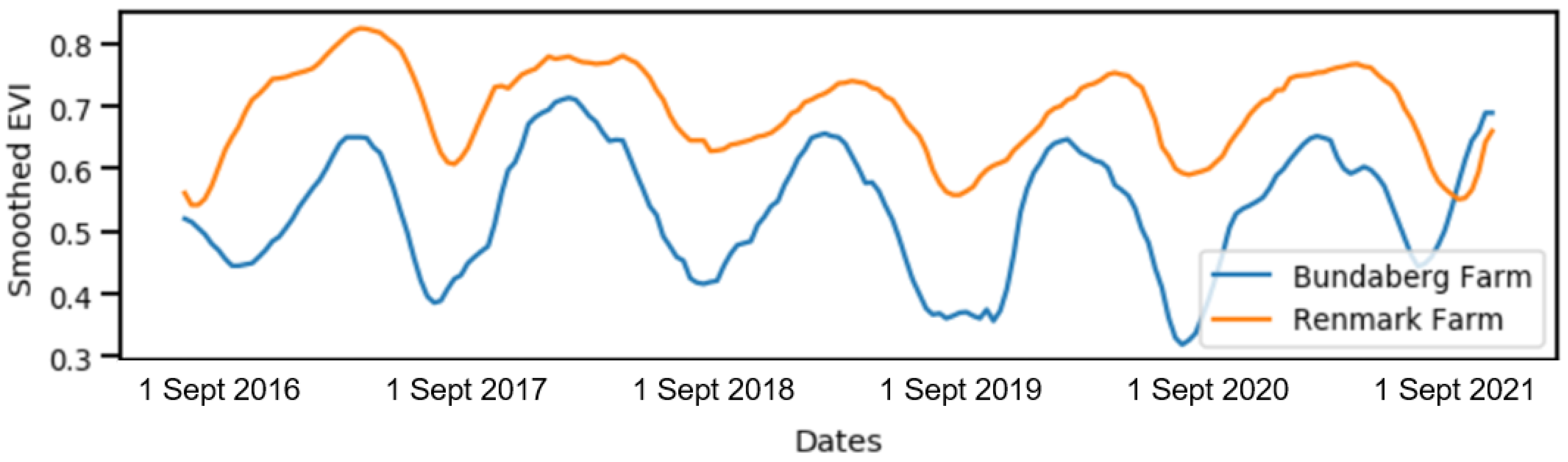
The variability in the EVI trends between the Bundaberg and Renmark avocado farms during the study period (2017–2021) is explored in Figure 8. Both curves showed similar trends, with a one- to two-week difference in the peak and trough. The EVI values for the Renmark farm were much higher (0.52 to 0.82) compared to those for the Bundaberg farm (0.3 to 0.73).
The Pearson correlation analysis of the EVI trends during the study period (2017–2021) for the Bundaberg and Renmark avocado farms did not show significant differences between the two farms, with R = 0.68 and p-value < 0.01. However, the Tukey-HSD test analysis (Table 4) showed significant difference between the mean EVI values between the two farms.
4. Discussion
In this study, S2-derived time-series EVI data were explored to understand the phenological profile of avocado crops over a five-year period (2017 to 2021) in the Bundaberg and Renmark regions of Australia. An SG filter was applied to smooth out the noise in the time-series EVI data. The trend lines in both regions showed a similar pattern over the study period (2017–2021), with a peak in June–July and a trough in September–October. However, slight deviations of two to three weeks were observed between the two regions, which could be due to different factors, such as weather conditions, crop age, and crop management practices [66], which might have been more precisely exposed in the EVI trends in both farms.
To describe the four key phenological stages (i.e., F, V, M, and H) with respect to the SG-smoothed time-series EVI data, the phenological events of avocado crops were defined according to calendar months. Two metrics derived from the SG-smoothed time-series EVI (EVImean and EVIslope) data clearly differentiated among the four phenological stages. In general, the seasonal time-series EVI (n = 5 years) followed a ‘sine’ curve, with a peak at the M stage and a trough at the F stage, which was similar to the findings reported by Torgbor, Rahman, Robson, Brinkhoff, and Khan [10] for mango crops. The minimum EVImean at the F stage could be due to the presence of flowers that reflected more in the green–red domain of the spectrum while causing no apparent changes in the blue and near-infrared (NIR) domain, which was reported by Shen et al. [67] and Torgbor, Rahman, Robson, Brinkhoff, and Khan [10]. Moreover, the simultaneous presence of both determinate and indeterminate inflorescence for the avocado crops and the fraction of canopy cover with flowers could have influenced the EVI trends at this stage. On the other hand, due to the simultaneous presence of developed shoots and fruits, the highest EVImean was observed at the M stage. The V and H stages resided on two opposite sides of the ‘sine’ curve, with comparable EVImean values. However, EVIslope differentiated between these two stages, since one had a positive slope and the other had negative. Due to the development of leaf flush and fruit set, the trend of EVI or EVIslope showed positive results in the V stage, whereas the crop harvest followed by pruning showed negative results in the H stage because of the declining biomass at this stage.
The most variability among the seasonal SG-smoothed EVI trends was witnessed in the F and V stages for both the Bundaberg and Renmark farms. The variation in the EVI at the F stage may be related to ‘alternate bearing’. Previous research [6,19,68] reported the loss of tens of thousands of avocado flowers at the F stage, which was not the same in the ‘on’ and ‘off’ seasons. Inter-annual variation at the V stage was also evident. This variability was due to the variation in shoot growth and fruit development at this stage, which has been reported by several previous researchers as well [65,69,70]. The higher value of the EVI at this stage could have been due to the greater vegetative growth and improved photosynthetic performance, which could lead to a high number of fruit sets, low fruit drop, and higher yield, and vice-versa [71,72].
According to the Pearson correlation analysis, there were no significant differences observed in the seasonal variability of the SG-smoothed EVI trends during the study period (2017–2021) for both the Bundaberg and Renmark avocado farms. Since the flowering in 2017 and 2020 in the Bundaberg farm started around two months later than in other years due to severe pruning events following the harvest in the previous season (from the growers’ data), the Pearson correlation analysis showed the lowest correlation between 2017 and 2021 (R = 0.63 and p-value < 0.01). In Renmark, the lowest correlations were observed in 2017–2019 and 2017–2020 (R = 0.8 and p-value < 0.01 in both years). However, the Tukey-HSD test showed significant inter-annual variability in the mean EVI values between years for both the Bundaberg and Renmark farms, which was predominantly due to the variations in the F and V stages, as discussed earlier. Future research on understanding the variability in the F and V stages in order to improve crop management, eliminate the ‘alternate bearing’ issue, and develop yield prediction models for avocado crops is warranted.
The Pearson correlation analysis of the EVI trends during the study period did not show any significant differences between the Bundaberg and Renmark avocado farms. However, the Tukey-HSD test showed a significant difference between the mean EVI values for the Bundaberg and Renmark avocado farms, which could be due to several factors, such as crop age, farm management practices, and weather (rainfall, temperature, relative humidity, etc.) [66].
5. Conclusions
To the best of our knowledge, the use of satellite remote sensing to describe avocado crop phenology is novel, although field studies for understanding the phenological changes in this crop have been conducted for more than two decades. In this study, S2-derived EVI data were explored to retrieve four key phenological stages (i.e., F, V, M, and H) of ‘Hass’ avocado crops in the Bundaberg and Renmark regions in Australia. The time-series EVI data that were studied over a 5-year period (2017–2021) showed seasonal variations that aligned favorably with phenological changes in avocado crops acquired from field observations. The combined use of EVImean and EVIslope differentiated among the four phenological stages in both farms. This information about phenological events from remote sensing data can provide a great benefit to the industry by guiding the key timings for crop management activities, including the application of crop inputs (e.g., nutrition, growth regulators, and fungicides, among others) and harvest scheduling without any labor-intensive and time-consuming field surveys. The variations in the EVI due to pruning in the Bundaberg farm demonstrated the potential of ‘benchmarking’ the seasonal trends of avocado crops, which can provide valuable information about significant variations resulting from pest and disease incursions and the potential impacts of seasonal weather variations. The potential use of very-high-resolution imagery, such as that from Planet Scope with 3 m spatial resolution and daily revisitation, could greatly improve the granularity and sensitivity of this form of orchard monitoring.
Author Contributions
M.M.R. conceived the idea and designed the research. M.M.R. conducted the experiments and drafted the manuscript. A.R. and J.B. revised the manuscript. M.M.R., A.R., and J.B. contributed to the scientific discussion of the article. All authors have read and agreed to the published version of the manuscript.
Funding
This research was funded by Horticulture Innovation Australia Ltd. (HIA), project number AV21006.
Acknowledgments
The authors of this paper would like to acknowledge the Horticulture Innovation Australia Ltd. (HIA) for funding this research, Avocado Australia Ltd. for their support, and Chad Simpson (Simpson Farms) for providing field-level avocado phenological data.
Conflicts of Interest
The authors declare no conflict of interest.
References
- Avocado Austrlia. Facts at a Glance for the Australian Avocado Industry—2020/21. 2021. Available online: https://avocado.org.au/wp-content/uploads/2021/10/2020-21_AAL-Facts-at-a-glance3.pdf (accessed on 30 July 2022).
- Whiley, A.W. Avocado Production in Australia. In Avocado Production in Asia and the Pacific; Papademtriou, M.K., Ed.; Food and Agriculture Organization of the United Nations, Regional Office for Asia and the Pacific: Bangkok, Thailand, 2000; Available online: https://www.fao.org/publications/card/en/c/e001af72-db59-5a89-ad40-aee479743100/ (accessed on 30 July 2022).
- Thorp, T.G.; Aspinall, D.; Sedgley, M. Preformation of Node Number in Vegetative and Reproductive Proleptic Shoot Modules of Persea (Lauraceae). Ann. Bot. 1994, 73, 13–22. [Google Scholar] [CrossRef]
- Whiley, A.W.; Wolstenholme, B.N. Carbohydrate management in avocado trees for increased production. SAAGA Yearb. 1990, 13, 25–27. [Google Scholar]
- Wolstenholme, B.N.; Whiley, A.W. Carbohydrate and phenological cycling as management tools for avocado orchards. SAAGA Yearb. 1989, 12, 33–37. [Google Scholar]
- Garner, L.C.; Lovatt, C.J. The Relationship Between Flower and Fruit Abscission and Alternate Bearing of ‘Hass’ Avocado. J. Am. Soc. Hortic. Sci. 2008, 133, 3–10. [Google Scholar] [CrossRef]
- Whiley, A.W.; Saranah, J.B.; Wolstenholme, B.N. Pheno-physiological modelling in avocado-an aid in research planning. In Proceedings of the World Avocado Congress III, Tel Aviv, Israel, 22–27 October 1995; pp. 71–75. [Google Scholar]
- Alcaraz, M.; Thorp, T.G.; Hormaza, J. Phenological growth stages of avocado (Persea americana) according to the BBCH scale. Sci. Hortic. 2013, 164, 434–439. [Google Scholar] [CrossRef]
- Márquez-Santos, M.; Hernández-Lauzardo, A.N.; Castrejón-Gómez, V.R. States of phenological development of avocado (Persea americana Mill.) based on the BBCH scale extended and its relationship to the incidence of anthracnose in field conditions. Sci. Hortic. 2020, 271, 109379. [Google Scholar] [CrossRef]
- Torgbor, B.A.; Rahman, M.M.; Robson, A.; Brinkhoff, J.; Khan, A. Assessing the Potential of Sentinel-2 Derived Vegetation Indices to Retrieve Phenological Stages of Mango in Ghana. Horticulturae 2022, 8, 11. [Google Scholar] [CrossRef]
- Salazar-García, S.; Lord, E.M.; Lovatt, C.J. Inflorescence and flower development of the ‘Hass’ avocado (Persea americana Mill.) during “on” and “off” crop years. J. Am. Soc. Hortic. Sci. 1998, 123, 537–544. [Google Scholar] [CrossRef] [Green Version]
- Chanderbali, A.S.; Soltis, D.E.; Soltis, P.S.; Wolstenholme, B.N. Taxonomy and botany. In The Avocado, Botany, Production and Uses; Schaffer, B., Wolstenholme, B.N., Whiley, A.W., Eds.; CAB International: Wallingford, UK, 2013; pp. 31–49. [Google Scholar]
- Thorp, T.G.; Sedgley, M. Architectural analysis of tree form in a range of avocado cultivars. Sci. Hortic. 1993, 53, 85–98. [Google Scholar] [CrossRef]
- Newett, S.; Dixon, J. Avocado Tree Growth Cycle. Available online: http://www.avocadosource.com/journals/ausnz/ausnz_2009/newettsimon2009.pdf (accessed on 30 September 2021).
- Bergh, B. Factors affecting avocado fruitfulness. In Proceedings of the First International Tropical Fruit Short Course: The Avocado; University of Florida: Gainesville, FL, USA, 1977; pp. 83–88. [Google Scholar]
- Wolstenholme, B.; Whiley, A. Strategies for maximising avocado productivity: An overview. In Proceedings of the World Avocado Congress III, Tel Aviv, Israel, 22–27 October 1995; p. 70. [Google Scholar]
- Dixon, J.; Elmsly, T.; Dixon, E.; Mandemaker, A.; Pak, H. Factors Influencing Fruit Set of Hass Avocados in New Zealand. In Proceedings of the World Avocado Congress VI, Viña del Mar, Chile, 12–16 November 2007; ISBN 978-956-17-0413-8. [Google Scholar]
- Lahav, E.; Zamet, D. Flowers, fruitlets and fruit drop in avocado trees. Rev. Chapingo Ser. Hortic. 1999, 5, 95–100. [Google Scholar]
- Garner, L.C.; Lovatt, C.J. Physiological factors affecting flower and fruit abscission of ‘Hass’ avocado. Sci. Hortic. 2016, 199, 32–40. [Google Scholar] [CrossRef]
- Kaiser, C.; Wolstenholme, B.N. Aspects of delayed harvest of ‘Hass’ avocado (Persea americana Mill.) fruit in a cool subtropical climate. I. Fruit lipid and fatty acid accumulation. J. Hortic. Sci. 1994, 69, 437–445. [Google Scholar] [CrossRef]
- Pinto, J.; Rueda-Chacón, H.; Arguello, H. Classification of Hass avocado (Persea americana mill) in terms of its ripening via hyperspectral images. TecnoLógicas 2019, 22, 111–130. [Google Scholar] [CrossRef]
- Toivonen, P.M.A.; Brummell, D.A. Biochemical bases of appearance and texture changes in fresh-cut fruit and vegetables. Postharvest Biol. Technol. 2008, 48, 1–14. [Google Scholar] [CrossRef]
- Piao, S.; Liu, Q.; Chen, A.; Janssens, I.A.; Fu, Y.; Dai, J.; Liu, L.; Lian, X.; Shen, M.; Zhu, X. Plant phenology and global climate change: Current progresses and challenges. Glob. Chang. Biol. 2019, 25, 1922–1940. [Google Scholar] [CrossRef] [PubMed]
- Usha, K.; Singh, B. Potential applications of remote sensing in horticulture—A review. Sci. Hortic. 2013, 153, 71–83. [Google Scholar] [CrossRef]
- Boschetti, M.; Stroppiana, D.; Brivio, P.A.; Bocchi, S. Multi-year monitoring of rice crop phenology through time series analysis of MODIS images. Int. J. Remote Sens. 2009, 30, 4643–4662. [Google Scholar] [CrossRef]
- Yang, W.; Zhang, S. Monitoring Vegetation Phenology Using MODIS Time-Series Data. In Proceedings of the 2012 2nd International Conference on Remote Sensing, Environment and Transportation Engineering, (RSETE), Nanjing, China, 1–3 June 2012; pp. 1–4. [Google Scholar]
- Pan, Z.; Huang, J.; Zhou, Q.; Wang, L.; Cheng, Y.; Zhang, H.; Blackburn, G.A.; Yan, J.; Liu, J. Mapping crop phenology using NDVI time-series derived from HJ-1 A/B data. Int. J. Appl. Earth Obs. Geoinf. 2015, 34, 188–197. [Google Scholar] [CrossRef] [Green Version]
- Zheng, Y.; Wu, B.; Zhang, M.; Zeng, H. Crop Phenology Detection Using High Spatio-Temporal Resolution Data Fused from SPOT5 and MODIS Products. Sensors 2016, 16, 2099. [Google Scholar] [CrossRef] [Green Version]
- Sehgal, V.K.; Jain, S.; Aggarwal, P.K.; Jha, S. Deriving Crop Phenology Metrics and Their Trends Using Times Series NOAA-AVHRR NDVI Data. J. Indian Soc. Remote Sens. 2011, 39, 373–381. [Google Scholar] [CrossRef]
- Shihua, L.; Jingtao, X.; Ping, N.; Jing, Z.; Hongshu, W.; Jingxian, W. Monitoring paddy rice phenology using time series MODIS data over Jiangxi Province, China. Int. J. Agric. Biol. Eng. 2014, 7, 28–36. [Google Scholar]
- Sun, L.; Gao, F.; Anderson, M.C.; Kustas, W.P.; Alsina, M.M.; Sanchez, L.; Sams, B.; McKee, L.; Dulaney, W.; White, W.A.; et al. Daily Mapping of 30 m LAI and NDVI for Grape Yield Prediction in California Vineyards. Remote Sens. 2017, 9, 317. [Google Scholar] [CrossRef] [Green Version]
- Sakamoto, T.; Yokozawa, M.; Toritani, H.; Shibayama, M.; Ishitsuka, N.; Ohno, H. A crop phenology detection method using time-series MODIS data. Remote Sens. Environ. 2005, 96, 366–374. [Google Scholar] [CrossRef]
- Brown, M.; De Beurs, K.; Marshall, M. Global phenological response to climate change in crop areas using satellite remote sensing of vegetation, humidity and temperature over 26 years. Remote Sens. Environ. 2012, 126, 174–183. [Google Scholar] [CrossRef]
- Heumann, B.W.; Seaquist, J.; Eklundh, L.; Jönsson, P. AVHRR derived phenological change in the Sahel and Soudan, Africa, 1982–2005. Remote Sens. Environ. 2007, 108, 385–392. [Google Scholar] [CrossRef]
- Pan, L.; Xia, H.; Zhao, X.; Guo, Y.; Qin, Y. Mapping Winter Crops Using a Phenology Algorithm, Time-Series Sentinel-2 and Landsat-7/8 Images, and Google Earth Engine. Remote Sens. 2021, 13, 2510. [Google Scholar] [CrossRef]
- Rahman, M.M.; Robson, A. Integrating Landsat-8 and Sentinel-2 Time Series Data for Yield Prediction of Sugarcane Crops at the Block Level. Remote Sens. 2020, 12, 1313. [Google Scholar] [CrossRef] [Green Version]
- Griffiths, P.; Nendel, C.; Hostert, P. Intra-annual reflectance composites from Sentinel-2 and Landsat for national-scale crop and land cover mapping. Remote Sens. Environ. 2019, 220, 135–151. [Google Scholar] [CrossRef]
- Rodrigues, A.; Marçal, A.R.; Cunha, M. Monitoring vegetation dynamics inferred by satellite data using the PhenoSat tool. IEEE Trans. Geosci. Remote Sens. 2012, 51, 2096–2104. [Google Scholar] [CrossRef]
- Duarte, L.; Teodoro, A.C.; Monteiro, A.T.; Cunha, M.; Gonçalves, H. QPhenoMetrics: An open source software application to assess vegetation phenology metrics. Comput. Electron. Agric. 2018, 148, 82–94. [Google Scholar] [CrossRef]
- Eklundh, L.; Jönsson, P. TIMESAT for Processing Time-Series Data from Satellite Sensors for Land Surface Monitoring. In Multitemporal Remote Sensing; Remote Sensing and Digital Image Processing; Ban, Y., Ed.; Springer: Cham, Switzerland, 2016; Volume 20. [Google Scholar] [CrossRef]
- Eerens, H.; Haesen, D.; Rembold, F.; Urbano, F.; Tote, C.; Bydekerke, L. Image time series processing for agriculture monitoring. Environ. Model. Softw. 2014, 53, 154–162. [Google Scholar] [CrossRef]
- Sawant, S.; Chakraborty, M.; Suradhaniwar, S.; Adinarayana, J.; Durbha, S. Time series analysis of remote sensing observtions for citrus crop growth stage and evapotranspiration estimation. In Proceedings of the International Archives of the Photogrammetry, Remote Sensing and Spatial Information Sciences, XXIII ISPRS Congress, Prague, Czech Republic, 12–19 July 2016; Volume XLI-B8. [Google Scholar] [CrossRef]
- Choudhary, K.; Shi, W.; Boori, M.S.; Corgne, S. Agriculture phenology monitoring using NDVI time series based on remote sensing satellites: A case study of Guangdong, China. Opt. Mem. Neural Netw. 2019, 28, 204–214. [Google Scholar] [CrossRef]
- Hatfield, J.L.; Gitelson, A.A.; Schepers, J.S.; Walthall, C.L. Application of spectral remote sensing for agronomic decisions. Agron. J. 2008, 100, S117–S131. [Google Scholar] [CrossRef] [Green Version]
- Fraga, H.; Amraoui, M.; Malheiro, A.C.; Moutinho-Pereira, J.; Eiras-Dias, J.; Silvestre, J.; Santos, J.A. Examining the relationship between the Enhanced Vegetation Index and grapevine phenology. Eur. J. Remote Sens. 2014, 47, 753–771. [Google Scholar] [CrossRef]
- Bai, T.; Zhang, N.; Mercatoris, B.; Chen, Y. Jujube yield prediction method combining Landsat 8 Vegetation Index and the phenological length. Comput. Electron. Agric. 2019, 162, 1011–1027. [Google Scholar] [CrossRef]
- Huete, A.; Didan, K.; Miura, T.; Rodriguez, E.P.; Gao, X.; Ferreira, L.G. Overview of the radiometric and biophysical performance of the MODIS vegetation indices. Remote Sens. Environ. 2002, 83, 195–213. [Google Scholar] [CrossRef]
- Galford, G.L.; Mustard, J.F.; Melillo, J.; Gendrin, A.; Cerri, C.C.; Cerri, C.E. Wavelet analysis of MODIS time series to detect expansion and intensification of row-crop agriculture in Brazil. Remote Sens. Environ. 2008, 112, 576–587. [Google Scholar] [CrossRef]
- Chen, J.; Jönsson, P.; Tamura, M.; Gu, Z.; Matsushita, B.; Eklundh, L. A simple method for reconstructing a high-quality NDVI time-series data set based on the Savitzky–Golay filter. Remote Sens. Environ. 2004, 91, 332–344. [Google Scholar] [CrossRef]
- Cao, R.; Chen, Y.; Shen, M.; Chen, J.; Zhou, J.; Wang, C.; Yang, W. A simple method to improve the quality of NDVI time-series data by integrating spatiotemporal information with the Savitzky-Golay filter. Remote Sens. Environ. 2018, 217, 244–257. [Google Scholar] [CrossRef]
- Chen, Y.; Cao, R.; Chen, J.; Liu, L.; Matsushita, B. A practical approach to reconstruct high-quality Landsat NDVI time-series data by gap filling and the Savitzky–Golay filter. ISPRS J. Photogramm. Remote Sens. 2021, 180, 174–190. [Google Scholar] [CrossRef]
- Meng, J.; Wu, B.; Li, Q.; Du, X.; Jia, K. Monitoring crop phenology with MERIS data—A case study of winter wheat in North China Plain. In Proceedings of the Progress in Electromagnetics Research Symposium, Beijing, China, 23–27 March 2009; pp. 1225–1228. [Google Scholar]
- BOM. Bureau of Meteorology. Available online: http://www.bom.gov.au (accessed on 15 September 2021).
- Gorelick, N.; Hancher, M.; Dixon, M.; Ilyushchenko, S.; Thau, D.; Moore, R. Google Earth Engine: Planetary-scale geospatial analysis for everyone. Remote Sens. Environ. 2017, 202, 18–27. [Google Scholar] [CrossRef]
- Pan, L.; Xia, H.; Yang, J.; Niu, W.; Wang, R.; Song, H.; Guo, Y.; Qin, Y. Mapping cropping intensity in Huaihe basin using phenology algorithm, all Sentinel-2 and Landsat images in Google Earth Engine. Int. J. Appl. Earth Obs. Geoinf. 2021, 102, 102376. [Google Scholar] [CrossRef]
- Louis, J.; Debaecker, V.; Pflug, B.; Main-Knorn, M.; Bieniarz, J.; Mueller-Wilm, U.; Cadau, E.; Gascon, F. Sentinel-2 Sen2Cor: L2A processor for users. In Proceedings of the Living Planet Symposium 2016, Prague, Czech Republic, 9–13 May 2016; pp. 1–8. [Google Scholar]
- Zhu, Z.; Woodcock, C.E. Automated cloud, cloud shadow, and snow detection in multitemporal Landsat data: An algorithm designed specifically for monitoring land cover change. Remote Sens. Environ. 2014, 152, 217–234. [Google Scholar] [CrossRef]
- Li, H.; Jia, M.; Zhang, R.; Ren, Y.; Wen, X. Incorporating the Plant Phenological Trajectory into Mangrove Species Mapping with Dense Time Series Sentinel-2 Imagery and the Google Earth Engine Platform. Remote Sens. 2019, 11, 2479. [Google Scholar] [CrossRef] [Green Version]
- Huete, A.R.; Liu, H.Q.; Batchily, K.; van Leeuwen, W. A comparison of vegetation indices over a global set of TM images for EOS-MODIS. Remote Sens. Environ. 1997, 59, 440–451. [Google Scholar] [CrossRef]
- Miura, T.; Huete, A.R.; Yoshioka, H.; Holben, B.N. An error and sensitivity analysis of atmospheric resistant vegetation indices derived from dark target-based atmospheric correction. Remote Sens. Environ. 2001, 78, 284–298. [Google Scholar] [CrossRef]
- Savitzky, A.; Golay, M.J. Smoothing and differentiation of data by simplified least squares procedures. Anal. Chem. 1964, 36, 1627–1639. [Google Scholar] [CrossRef]
- Beurs, K.M.d.; Henebry, G.M. Spatio-temporal statistical methods for modelling land surface phenology. In Phenological Research; Hudson, I., Keatley, M., Eds.; Springer: Dordrecht, The Netherlands, 2010; pp. 177–208. [Google Scholar] [CrossRef]
- Bressert, E. SciPy and NumPy: An overview for Developers; O’Reilly Media, Inc.: Sebastopol, CA, USA, 2012. [Google Scholar]
- Van Rossum, G.; Drake, F.L. Python 3 Reference Manual; CreateSpace: Scotts Valley, CA, USA, 2009. [Google Scholar]
- Liu, X.; Hofshi, R.; Arpaia, M.L. Hass’ avocado leaf growth, abscission, carbon production and fruit set. In Proceedings of the Avocado Brainstorming, Riverside, CA, USA, 27–28 October 1999; Arpaia, M.L., Hofshi, R., Eds.; Hofshi Foundation: Fallbrook, CA, USA, 1999; pp. 52–55. [Google Scholar]
- Basso, B.; Cammarano, D.; Carfagna, E. Review of crop yield forecasting methods and early warning systems. In Proceedings of the First Meeting of the Scientific Advisory Committee of the Global Strategy to Improve Agricultural and Rural Statistics, Rome, Italy, 9–10 April 2013; p. 19. [Google Scholar]
- Shen, M.; Chen, J.; Zhu, X.; Tang, Y. Yellow flowers can decrease NDVI and EVI values: Evidence from a field experiment in an alpine meadow. Can. J. Remote Sens. 2009, 35, 99–106. [Google Scholar] [CrossRef]
- Inoue, H.; Takahashi, B. Studies on the Bearing Behavior and Yield Composition of the Avocado Tree. J. Jpn. Soc. Hortic. Sci. 1990, 59, 487–501. [Google Scholar] [CrossRef]
- Davenport, T. Avocado growth and development. Proc. Fla. State Hortic. Soc. 1982, 95, 92–96. [Google Scholar]
- Mickelbart, M.V.; Robinson, P.W.; Witney, G.; Arpaia, M.L. ‘Hass’ avocado tree growth on four rootstocks in California. II. Shoot and root growth. Sci. Hortic. 2012, 143, 205–210. [Google Scholar] [CrossRef]
- Whiley, A.W.; Saranah, J.B.; Rasmussen, T.S. The Relationship between Carbohydrate Levels and Productivity in the Avocado and Impact on Management Practices, Particularly Time of Harvest; Talking Avocados, Report—AV033; Queensland Department of Primary Industries: Brisbane, Australia, 1996. [Google Scholar]
- Wolstenholme, B. Theoretical and applied aspects of avocado yield as affected by energy budgets and carbon partitioning. In South African Avocado Growers’ Association Yearbook, Proceedings of the First World Avocado Congress, Pretoria, South Africa, 4–8 May 1987; South African Avocado Growers’ Association: Tzaneen, South Africa, 1987; Volume 10, pp. 58–61. [Google Scholar]
Figure 1.
Locations of the four avocado blocks in Bundaberg, Queensland and the three avocado blocks in Renmark, South Australia.
Figure 1.
Locations of the four avocado blocks in Bundaberg, Queensland and the three avocado blocks in Renmark, South Australia.

Figure 2.
Monthly averages of the maximum (Tmax) and minimum (Tmin) air temperatures (°C), along with the monthly average rainfall (mm) for the Bundaberg (top) and Renmark (bottom) study regions (2001–2021).
Figure 2.
Monthly averages of the maximum (Tmax) and minimum (Tmin) air temperatures (°C), along with the monthly average rainfall (mm) for the Bundaberg (top) and Renmark (bottom) study regions (2001–2021).

Figure 3.
Avocado phenological stages in (a) Bundaberg and (b) Renmark (data acquired from the growers).
Figure 3.
Avocado phenological stages in (a) Bundaberg and (b) Renmark (data acquired from the growers).

Figure 4.
The workflow for monitoring avocado crop phenological stages using time-series Sentinel 2 images.
Figure 4.
The workflow for monitoring avocado crop phenological stages using time-series Sentinel 2 images.

Figure 5.
Savitzky–Golay (SG)-smoothed curve fitted to Sentinel 2 (S2) time-series EVI data over five years (2017–2021) for the (a) Bundaberg (four blocks) and (b) Renmark (three blocks) avocado farms. The four different colors show the four phenological stages (i.e., F, V, M, and H) according to the calendar months.
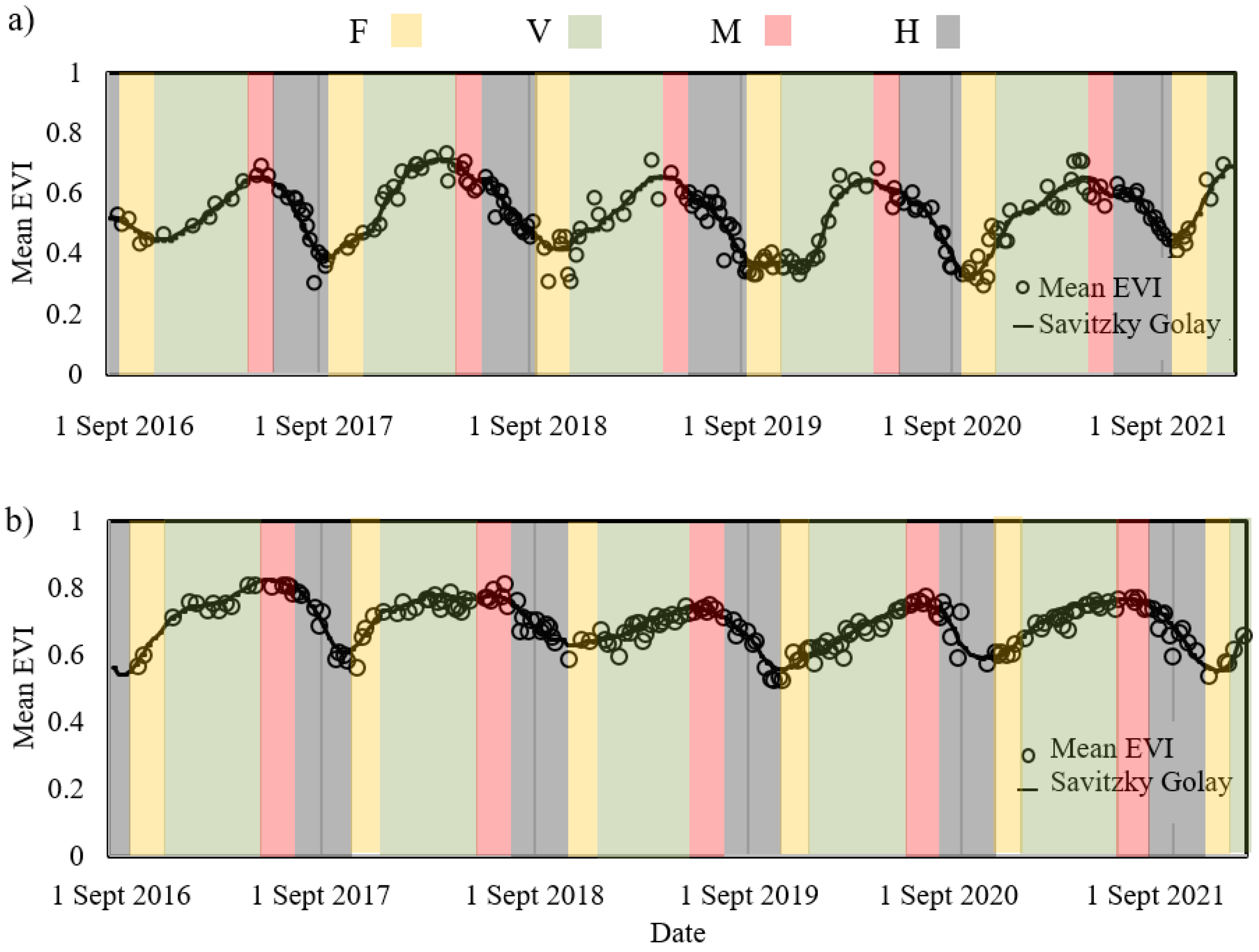
Figure 6.
The box plots of EVImean and EVIslope data showing the differences among the four phenological stages (i.e., F, V, M, and H) for the (a) Bundaberg (n = 5 years) and (b) Renmark (n = 5 years) avocado farms.
Figure 6.
The box plots of EVImean and EVIslope data showing the differences among the four phenological stages (i.e., F, V, M, and H) for the (a) Bundaberg (n = 5 years) and (b) Renmark (n = 5 years) avocado farms.
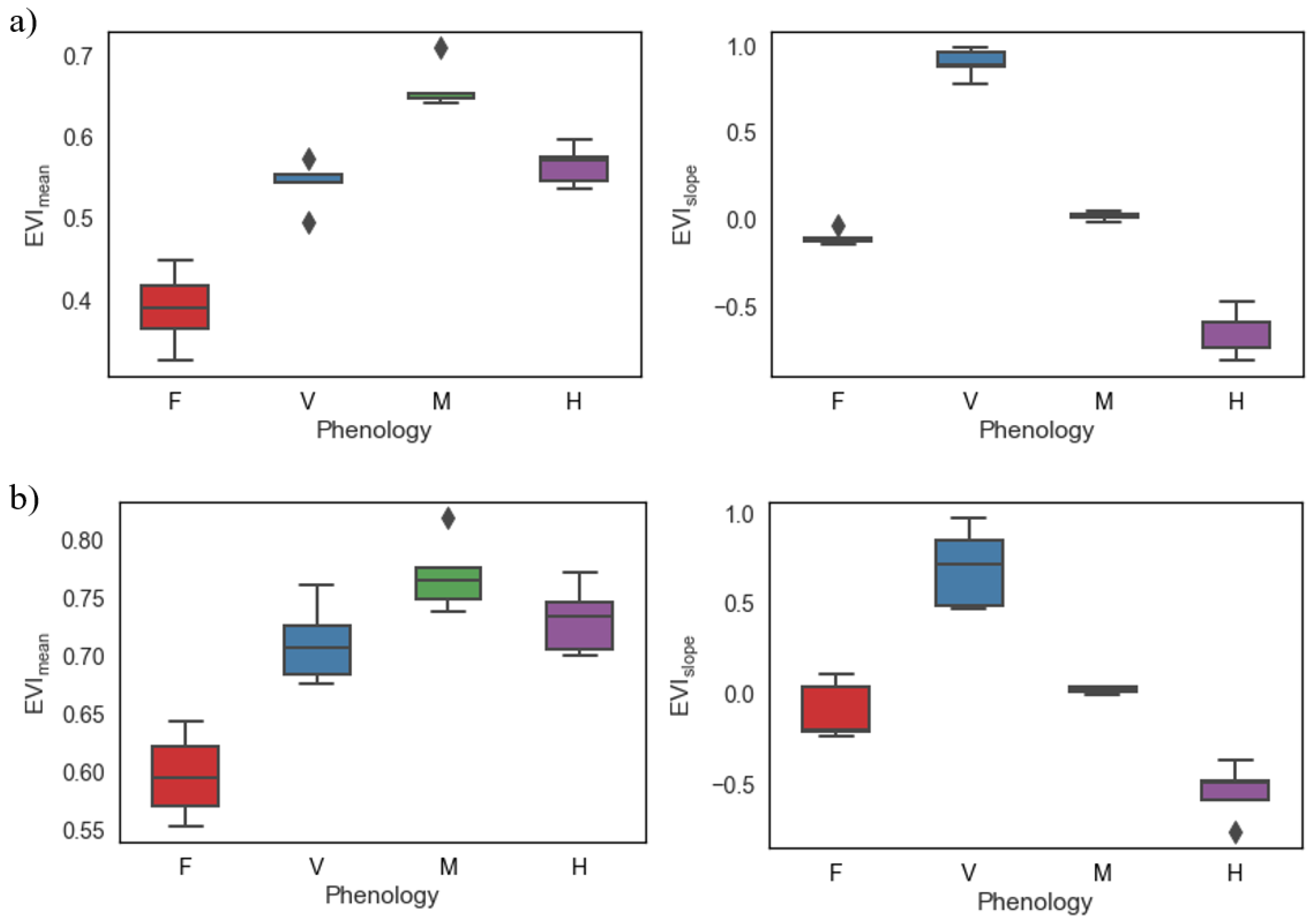
Figure 7.
Seasonal variations in EVI trends within the study period (2017–2021) in the (a) Bundaberg and (b) Renmark avocado farms.
Figure 7.
Seasonal variations in EVI trends within the study period (2017–2021) in the (a) Bundaberg and (b) Renmark avocado farms.
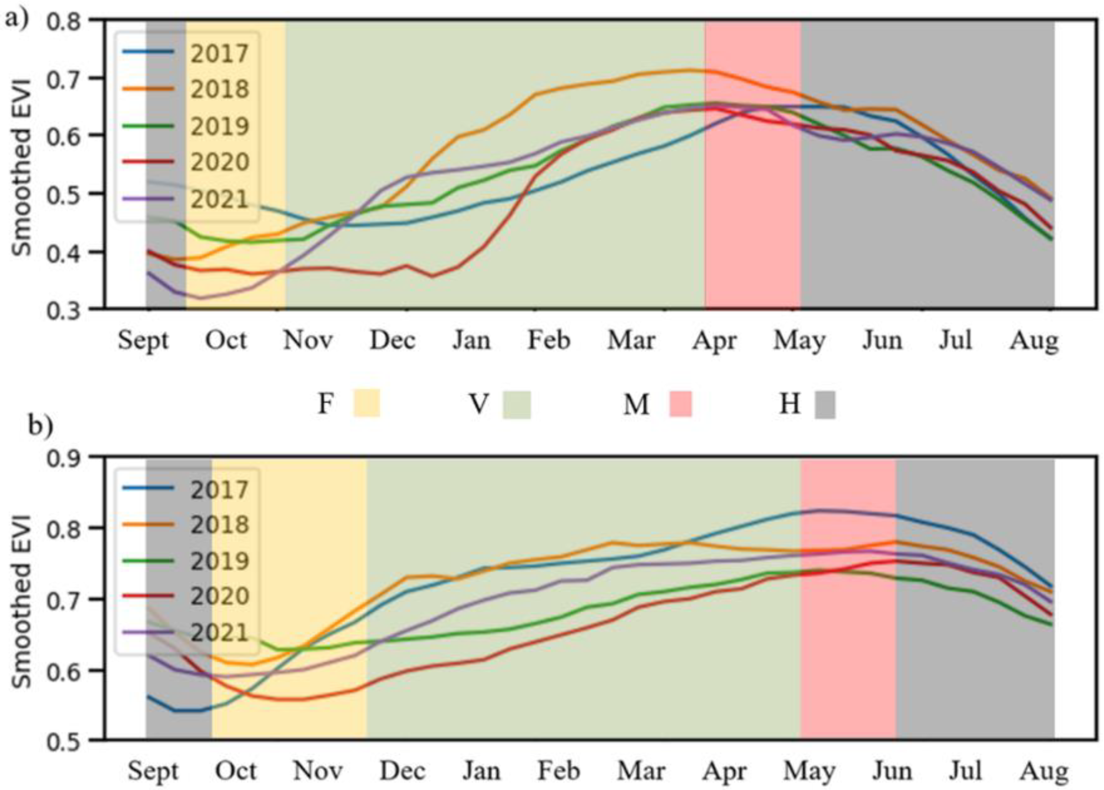
Figure 8.
Temporal variability of the EVI trends between the Bundaberg and Renmark avocado farms.

Table 1.
The four avocado phenological stages in Bundaberg and Renmark.
| Phenology Stages | Bundaberg | Renmark |
|---|---|---|
| Flowering (F) | September 2nd week–October 3rd week | September 3rd week–November 3rd week |
| Vegetative flush (V) | October 4th week–April | November 4th week–May |
| Fruit Maturity (M) | April–May | May–June |
| Harvest (H) | May–September 1st week | June–September 2nd week |
Table 2.
Results of the Tukey-HSD test on the phenological stages for the Bundaberg and Renmark farms.
Table 2.
Results of the Tukey-HSD test on the phenological stages for the Bundaberg and Renmark farms.
| EVImean at Bundaberg Farm | ||||
|---|---|---|---|---|
| Difference between Stages | Mean Difference | Std. Error | t | P > |t| |
| H-F | 0.18 | 0.02 | 8.30 | 3.39 × 10⁻⁷ |
| M-F | 0.28 | 0.02 | 12.80 | 8.02 × 10⁻¹⁰ |
| V-F | 0.16 | 0.02 | 7.22 | 2.04 × 10⁻⁶ |
| M-H | 0.10 | 0.02 | 4.49 | 3.67 × 10⁻⁴ |
| V-H | −0.03 | 0.02 | −1.08 | 2.94 × 10⁻¹ |
| V-M | −0.12 | 0.02 | −5.58 | 4.14 × 10⁻⁵ |
| EVIslope at Bundaberg Farm | ||||
| H-F | −0.56 | 0.05 | −10.61 | 1.20 × 10⁻⁸ |
| M-F | 0.12 | 0.05 | 2.29 | 3.58 × 10⁻² |
| V-F | 1.00 | 0.05 | 18.86 | 2.35 × 10⁻¹² |
| M-H | 0.69 | 0.05 | 12.90 | 7.16 × 10⁻¹⁰ |
| V-H | 1.57 | 0.05 | 29.47 | 2.27 × 10⁻¹⁵ |
| V-M | 0.88 | 0.05 | 16.57 | 1.70 × 10⁻¹¹ |
| EVImean at Renmark Farm | ||||
| H-F | 0.13 | 0.02 | 6.39 | 8.81 × 10⁻⁶ |
| M-F | 0.17 | 0.02 | 8.18 | 4.12 × 10⁻⁷ |
| V-F | 0.11 | 0.02 | 5.41 | 5.74 × 10⁻⁵ |
| M-H | 0.04 | 0.02 | 1.78 | 9.32 × 10⁻² |
| V-H | −0.02 | 0.02 | −0.98 | 3.39 × 10⁻¹ |
| V-M | −0.06 | 0.02 | −2.77 | 1.36 × 10⁻² |
| EVIslope at Renmark Farm | ||||
| H-F | −0.44 | 0.09 | −4.48 | 3.79 × 10⁻⁴ |
| M-F | 0.12 | 0.09 | 1.21 | 2.45 × 10⁻¹ |
| V-F | 0.79 | 0.09 | 8.11 | 4.66 × 10⁻⁷ |
| M-H | 0.56 | 0.09 | 5.68 | 3.38 × 10⁻⁵ |
| V-H | 1.24 | 0.09 | 12.59 | 1.03 × 10⁻⁹ |
| V-M | 0.68 | 0.09 | 6.90 | 3.57 × 10⁻⁶ |
Table 3.
Results of the Tukey-HSD test for the Bundaberg and Renmark avocado farms.
| Bundaberg Farm | ||||
|---|---|---|---|---|
| Difference between Stages | Mean Difference | Std. Error | t | P > |t| |
| 2017–2018 | −0.043506 | 0.023061 | −1.886572 | 0.366870 |
| 2017–2019 | 0.000944 | 0.023061 | 0.040955 | 0.998689 |
| 2017–2020 | 0.035722 | 0.023061 | 1.549056 | 0.545558 |
| 2017–2021 | 0.003178 | 0.023061 | 0.137801 | 0.998689 |
| 2018–2019 | −0.044450 | 0.023061 | −1.927527 | 0.366870 |
| 2018–2020 | −0.079228 | 0.023061 | −3.435628 | 0.007359 * |
| 2018–2021 | −0.046683 | 0.023061 | −2.024373 | 0.335841 |
| 2019–2020 | −0.034778 | 0.023061 | −1.508101 | 0.545558 |
| 2019–2021 | −0.002233 | 0.023061 | −0.096846 | 0.998689 |
| 2020–2021 | 0.032544 | 0.023061 | 1.411255 | 0.545558 |
| Renmark Farm | ||||
| 2017–2018 | −0.002528 | 0.015251 | −0.165742 | 0.868552 |
| 2017–2019 | 0.042694 | 0.015251 | 2.799396 | 0.039189 * |
| 2017–2020 | 0.063444 | 0.015251 | 4.159935 | 0.000448 * |
| 2017–2021 | 0.027539 | 0.015251 | 1.805674 | 0.260559 |
| 2018–2019 | −0.045222 | 0.015251 | −2.965137 | 0.027252 * |
| 2018–2020 | −0.065972 | 0.015251 | −4.325676 | 0.000255 * |
| 2018–2021 | −0.030067 | 0.015251 | −1.971416 | 0.227248 |
| 2019–2020 | −0.020750 | 0.015251 | −1.360539 | 0.439319 |
| 2019–2021 | 0.015156 | 0.015251 | 0.993722 | 0.539950 |
| 2020–2021 | 0.035906 | 0.015251 | 2.354261 | 0.112360 |
* Statistically significant difference between means with p-value < 0.05.
Table 4.
Tukey-HSD test between the Bundaberg and Renmark avocado farms.
| EVImean at Bundaberg Farm | ||||
|---|---|---|---|---|
| Difference between Farms | Mean Difference | Std. Error | t | P > |t| |
| Renmark–Bundaberg | 0.16 | 0.01 | 18.00 | 4.09 × 10−53 |
Publisher’s Note: MDPI stays neutral with regard to jurisdictional claims in published maps and institutional affiliations. |
© 2022 by the authors. Licensee MDPI, Basel, Switzerland. This article is an open access article distributed under the terms and conditions of the Creative Commons Attribution (CC BY) license (https://creativecommons.org/licenses/by/4.0/).
Share and Cite
MDPI and ACS Style
Rahman, M.M.; Robson, A.; Brinkhoff, J. Potential of Time-Series Sentinel 2 Data for Monitoring Avocado Crop Phenology. Remote Sens. 2022, 14, 5942. https://doi.org/10.3390/rs14235942
AMA Style
Rahman MM, Robson A, Brinkhoff J. Potential of Time-Series Sentinel 2 Data for Monitoring Avocado Crop Phenology. Remote Sensing. 2022; 14(23):5942. https://doi.org/10.3390/rs14235942
Chicago/Turabian StyleRahman, Muhammad Moshiur, Andrew Robson, and James Brinkhoff. 2022. "Potential of Time-Series Sentinel 2 Data for Monitoring Avocado Crop Phenology" Remote Sensing 14, no. 23: 5942. https://doi.org/10.3390/rs14235942
Note that from the first issue of 2016, this journal uses article numbers instead of page numbers. See further details here.