Regulation of Evapotranspiration in Different Precipitation Zones and Its Application in High-Temperature and Drought Monitoring

Abstract

When drought occurs in different regions, evapotranspiration (ET) changes differently with the process of drought. To achieve an accurate monitoring of large-scale drought using remote sensing, it is particularly necessary to clarify the temporal and spatial characteristics of ET changes with soil water content (SWC). Firstly, based on the measured data, combined with the artificial intelligence particle swarm optimization (PSO) algorithm, an empirical model of ET retrieval by FY–4A satellite data was established and the spatial–temporal characteristics of ET changes with SWC were further analyzed. Lastly, different ET regulation regions were distinguished to achieve the remote sensing monitoring of large-scale drought based on SWC. The main results are as follows: (1) The correlation coefficient between the ET estimated by the empirical model and the measured value was 0.48 and the root mean square error was 24 W·m⁻². (2) In the areas with extreme water shortage, water limits the conversion rate of net radiation (Rn) to ET (ECR) and surpasses Rn to become the determinative factor of ET. (3) In extreme arid areas, ET has a significant positive correlation with WVP and SWC. In other precipitation areas, ET has a significant linear correlation with WVP, but the slope of the linear fitting line is different for precipitation. The relationship between ET and SWC is more complex. In areas with precipitation exceeding 800 mm, the correlation between SWC and ET is not significant. In areas with precipitation between 200 mm and 800 mm or in alpine regions, SWC and ET have a quadratic relationship. (4) ECR has quadratic correlations with WVP and SWC, and ECR reaches the maximum when WVP = 0.182 kPa and SWC = 0.217 m³∙m⁻³. ET may be inhibited for water shortage or water supersaturation. (5) In areas where SWC determines ET, the ET stress index (ESI) is inversely proportional to SWC, and in areas where heat affects ET, the ESI is directly proportional to SWC. Therefore, for the accurate monitoring of large-scale drought, various drought monitoring criteria should be determined in different areas and periods, considering information on precipitation, the underlying surface type, and digital elevation.

1. Introduction

Drought is a meteorological disaster with the highest frequency, the longest duration, and the most extensive impact [1]. It has a profound impact on global agricultural production, ecological environment, and social and economic development [2]. The declaration of the “High-level Meeting on National Drought Policy” held by the United Nations in 2013 indicated that drought poses severe challenges to all countries in the world, especially in developing and the least developed countries, in terms of food security, poverty, lack of resources, deterioration of ecological environment, and social unrest. In the context of global climate change and increasing human activity, the frequency, intensity, and duration of drought are likely to increase. To respond to and manage drought better, reduce drought vulnerability, and avoid the series of impacts generated by drought, improvements in the monitoring of drought levels and early warning technology are important in the international drought research field [3].

Drought monitoring entails monitoring water conditions using data, such as precipitation, temperature, evapotranspiration (ET), and runoff which can be obtained from ground observation [4], satellite detection [5] and numerical models [6]. In recent decades, with the development of global Earth observation technology, drought monitoring technology has seen great progress. Various drought (or soil moisture) monitoring models and indexes have been developed, which have been effectively applied in drought monitoring in different countries [7,8,9,10,11,12,13,14,15,16].

However, the characteristics of drought differ greatly in temporal and spatial aspects, and drought has a strong variability, which makes the monitoring methods suitable for one area not applicable in other areas. Moreover, drought is difficult to monitor accurately on a large scale [17,18,19,20]. In view of the strong spatiotemporal heterogeneity of drought characteristics, the accuracy of drought monitoring is improved by developing various monitoring criteria [21].

As a key factor of energy and water balance, ET is a linking parameter between soil water content (SWC) and atmospheric water vapor through complex physical and physiological processes [22]. Measuring the water condition of the earth–atmosphere system is an important factor and one of the main parameters of drought monitoring. It plays an important role in hydrology, meteorology, and agriculture [23,24].

ET mainly includes crop transpiration and soil evaporation, which are closely related to the conditions of soil, crop, and atmosphere [25,26]. However, given the differences in regional precipitation, the water and heat characteristics of the soil, the underlying surface types, and crop drought resistance, the spatial and temporal differences of regulating factors and models are significant, which makes the characteristics of ET vary in different areas and periods and brings uncertainty to large-scale drought monitoring [27].

In view of the temporal and spatial differences of ET and the complexity of drought process, to improve the accuracy of large-scale drought monitoring, the determinative factors of ET in different regions and periods must be determined as well as the regulating rules of these factors.

On the basis of the observation data of 15 ground sites in China for years, this study discusses the determinative regulating factors of ET in different precipitation zones and periods, analyzes the variation characteristics of ET and parameters related with atmospheric and soil moisture, lays a foundation for the application of ET in atmospheric and soil water monitoring, and provides a basis for developing criteria for the division and monitoring of drought areas.

2. Materials and Methods

2.1. Materials

2.1.1. Introduction of Ground Sites

The observation data used in this study were obtained from the National Ecological Science Data Center (NESDC) (http://www.cnern.org.cn/index.jsp, accessed on 8 May 2020), National Tibetan Plateau Data Center (NTPDC) (https://data.tpdc.ac.cn/zh-hans/, accessed on 27 July 2021), Lanzhou University (http://www.lzu.edu.cn/, accessed on 1 April 2012), and Institute of Arid Meteorology. The data include air temperature (Ta), precipitation, net radiation (Rn), water vapor pressure (WVP), SWC, and the latent heat flux (LE) measured by eddy correlation method [28], and the data were collected once every 30 min. For more details of these data, refer to the introduction on the data website. The geographical locations of the observation sites are shown in Figure 1. The overview of the observation sites is shown in

Table 1. Overview of the observation sites used for developing the ET retrieval model.

Name	Site	Longitude (°E), Latitude (°N)	Vegetation Type	Observation Time	Application
Arou	AR	100.46, 38.05	Grassland	2020	Modeling
Jingyangling	JYL	101.12, 37.84	Grassland	2019	Modeling
Sidaoqiao	SDQ	101.14, 42.0	forest	2020	Modeling
Dingxi	DXX	104.58, 35.57	Cropland	2019–2020	Modeling (2019)/Verifying (2020)
Daman	DM	100.37, 38.86	Cropland	2019–2020	Verifying
Dashalong	DSL	98.94, 38.84	Grassland	2020	Verifying

and

Table 2. Overview of the observation sites used for ET regulation.

NO.	Name	Site	Longitude (°E), Latitude (°N)	Vegetation Type	Rainfall (mm)	Observation Time
1	Changbaishan	CBS	128.06, 42.24	Mixed forest	438–523	2003–2010
2	Dangxiong	DX	91.03, 30.29	Alpine meadow	241–648	2004–2010
3	Dinghushan	DHS	112.30, 23.09	Forest	1063–1989	2003–2010
4	Haibei	HB	101.20, 37.40	Alpine meadow	342–546	2003–2010
5	Neimeng	NM	116.18, 44.08	Grassland	107–364	2004, 2005, 2008–2010
6	Qianyanzhou	QYZ	115.03, 26.44	Forest	855–1454	2003–2010
7	Xishuangbanna	XSBN	101.16, 21.54	Forest	552–3458	2003–2010
8	Yuzhong	SACOL	104.13, 35.95	Grassland	225–402	2007–2010
9	Shiquanhe	SQH	80.08, 32.50	Desert	48–129	2014–2016

.

The purpose of the observation data is determined from the availability of the observation data, the geographical location of the station, and the observation period. Since the data released by FY–4A satellite began in 2018, the observation data of NTPDC with relatively short observation period and observation time after 2018 were selected as the data source for the development of the ET retrieval model, as shown in Table 1. In order to analyze the ET regulation mechanism, long–term observation data in different climatic regions and different underlying surfaces were required. Therefore, 9 stations distributed in different climatic regions along with the observation period were used for the analysis of the regulation mechanisms, as shown in Table 2.

2.1.2. Remote Sensing Data

The satellite remote sensing data used in this paper included Fengyun–4A/Advanced Geosynchronous Radiation Imager (FY–4A/AGRI) and Global Change Observation Mission 1st–Water/Advanced Microwave Scanning Radiometer–2 (GCOM–W1/AMSR–2) data. The FY–4A satellite remote sensing data were provided by the National Satellite Meteorological Center (http://www.nsmc.org.cn/NSMC/Home/Index.html, accessed on 31 August 2022), including level 1 products from 1 January 2019 to 31 August 2022, with a 4 km resolution. The data of soil moisture were from https://search.earthdata.nasa.gov/search, accessed on 31 August 2022, from 1 May 2013 to 31 August 2022, with a 10 km resolution.

2.1.3. Data Processing

(1) Data calculation

The daily, monthly, and annual precipitation (the unit is mm) were derived using 30 min data.

The daily, monthly, and annual average values of Ta, Ts, WVP, SWC, LE, and Rn were calculated using an average method based on 30 min data, with the units of °C, °C, kPa, m³∙m⁻³, W∙m⁻² and W∙m⁻², respectively.

(2) ET, TE, and LE

The ET used in this study can be expressed in two ways, TE and LE. TE is the total ET, which is the total amount of water vapor transport over a certain time scale, with the unit of mm. LE is the latent heat flux, which is a quantity of water vapor transport speed, with unit of W∙m⁻². TE = λ LE, where λ is the latent heat of vaporization, with λ = 2.45 MJ·kg⁻¹; 1 W∙m⁻² = 0.035 mm in daily time scale.

(3) The monthly cumulative rainfall and TE

The cumulative rainfall or TE in N month (CX_N) was calculated as follows:

$${\mathrm{CX}}_{\mathrm{N}}={{\displaystyle \sum }}_{\mathrm{i}=1}^{\mathrm{i}=\mathrm{N}}{\mathrm{CX}}_{\mathrm{i}},$$

(1)

where CX_i was the rainfall or TE in i month.

(4) Valid data filtering

The analysis of ET regulation uses monthly data. According to the calculation of corresponding observation periods of all sites, 696 research samples were expected in this paper. Through simple screening, which is mainly to eliminate unqualified data (e.g., invalid data and negative data of LE and Rn), 600 effective research samples were finally obtained. The missing data and retention period are shown in Figure 2.

The missing data of CBS, DX, DHS, HB, and NM sites are the data with negative values of LE and Rn in winter, and the invalid data of SWC and precipitation, with data retention percentage of 87%. The observation values of SACOL from September to December 2010 are missing, as well as the SQH data in June 2014.

(5) Remote sensing data

First, the FY–4A/AGRI remote sensing data were processed by geographic location and calibration to obtain the reflectance and brightness temperature. The point remote sensing data corresponding to the ground station was obtained by the nearest–neighbor interpolation method. Ten–day scale products were obtained by synthesizing the maximum of daily land surface temperature (LST), ET and ET stress index (ESI) results.

The daily, 10–day, and monthly average values of GCOM–W1/AMSR–2 were calculated by using the data of the ascending and descending orbits. The spatial resolutions of the two remote sensing data were unified to 4 km.

2.2. Methods

2.2.1. ET Retrieval

Research shows that remote sensing parameters closely related to ET can be combined with Rn to establish an estimation model to achieve ET retrieval [29]. The correlation analysis of ET/Rn and parameters is shown in Figure 3. The ratio of ET/Rn has the most significant correlation with the normalized difference vegetation index (NDVI) than average LST (LSTm) and the range of LST difference (DLSTR). Therefore, we used these parameters to develop an all–weather remote sensing retrieval model of the daily average ET in this study, that is,

$$\mathrm{ETv}={\mathrm{R}}_{\mathrm{n}}\left({\mathrm{a}}_0+{\mathrm{a}}_1\mathrm{NDVI}+{\mathrm{a}}_2\mathrm{LSTm}+{\mathrm{a}}_3\mathrm{DLSTR}\right),$$

(2)

where a₀–a₃ are the model coefficients obtained by the particle swarm optimization (PSO) algorithm [30] using the observation data of the stations in Table 1. The coefficients are 0.103, 0.06, 0.0043, and −0.0003, respectively. In this paper, the low and high LSTs were taken as the values at 8:00 after sunrise in the morning and 14:00 in the afternoon, respectively. LSTs at 8:00 and 14:00 were estimated by the algorithm developed by Becker and Li [31] with the modified emissivity model [26]. The Rn was retrieved by the model developed by Wang for FY–4A/AGRI data [32].

2.2.2. Estimation of the Potential ET

The ET calculated by the Priestley–Taylor method (PET) [33] is the lower limit of the ET intensity of moist underlying surface. PET is obtained by gradient transport theory and energy conservation principle under the conditions of wide and wet (saturated) underlying surface, ignoring boundary effect and advection. The difference between ET and PET can reflect the difference between the water condition and water saturation of the underlying surface [34]. The PET formula is as follows:

$$\mathrm{PET}=\mathsf{\alpha }\frac{∆}{∆+\mathsf{\gamma }}\left(\mathrm{Rn}-{\mathrm{G}}_0\right),$$

(3)

where Δ represents the slope of the vapor pressure–temperature curve. On the regional scale, PET is estimated by replacing the daily average air temperature with daily LSTm. γ represents the dry/wet bulb constant and α is the ratio between the actual evaporation and the equilibrium evaporation rate, in this study, α = 1.26. G₀ is the soil heat flux [35].

2.2.3. ESI

Studies have shown that the PET equation can estimate the ET of wet area. According to the symmetric complementary model [36], the difference between ET and PET under the condition of limited water can reflect the water content of the underlying surface. The common drought monitoring index based on ET is the ESI, which is expressed as follows:

$$\mathrm{ESI}=1-\mathrm{ET}/\mathrm{PET},$$

(4)

3. Results

3.1. ET Estimated Result

The diurnal ET estimated by Equation (2) using the FY–4A/AGRI data was shown in Figure 4. A significantly positive correlation exists between the estimated ET and the measured value. The correlation coefficient R² was 0.48, the root mean square error was 24 W·m⁻², and the slope of the fitting line was 1.07. This empirical model does not need the auxiliary input of ground observation data, and it can quickly achieve the remote sensing retrieval of ET on a large-scale. For regions and periods lacking ground observation data, the empirical model can effectively estimate the ET on a large-scale, and the estimation results have a certain credibility.

3.2. Time Series of Parameter Change

The time series of different parameters in the nine observation sites used for the ET regulation analysis are shown in Figure 5. Figure 5a shows the time series of Ta and precipitation. The Ta at each site has significant annual variation characteristics, and it reaches the highest in summer. The temperatures of the three sites in the tropics (XSBN) and subtropics (DHS and QYZ) are significantly higher than those in the other zones. The temperatures of the three sites in the tropics and subtropics are mainly in the range of 5 °C–30 °C. The temperatures of the three observation sites in the temperate zone (CBS, NM, and SACOL) range from −20 °C to 20 °C, and the temperatures of the three observation sites in the alpine zone (DX, HB, and SQH) range from −15 °C to 15 °C. The rising temperatures in the observation sites are all accompanied by increases in precipitation. All sites belong to the same period of rainfall and heat. Combined with Figure 5d, with the accumulation of precipitation, ET increases. However, since all stations are located where rainfall and high temperature occur at the same time, whether heat or water is dominant in the process of increasing ET needs to be further analyzed.

Figure 5b shows the time series of SWC and WVP at each observation site. Combined with the energy changes shown in Figure 5c, the results show that the WVPs of DHS, QYZ, and XSBN always have high levels, indicating that the atmosphere in these areas is in a relatively humid state, and the main energy change is ET. The SWCs of DX, NM, SACOL, and SQH sites always have low levels, especially, SQH (which is in the extreme water shortage zone), SWC, and WVP are have low levels. In terms of energy change, the energy distribution of DX, NM, and SACOL is seasonal, which mainly corresponds to precipitation. In the period of sufficient precipitation, SWC is high, and the energy distribution is dominated by ET. On the contrary, the energy distribution is mainly Hs. In SQH, where the atmosphere and soil are extremely dry, the difference of LST and Ta is large, and the energy distribution is mainly Hs. Before the precipitation season, the energy distribution of CBS and HB is mainly Hs, and after sufficient precipitation, the energy distribution of CBS and HB is mainly ET.

3.3. ET Regulation

The environmental factors affecting ET mainly associated with two aspects, namely, heat and water. The heat of the earth–atmosphere system originates from radiation. The radiation entering the earth–atmosphere system is expressed by Rn, and the increase in system heat is expressed by Ta. The water in the earth–atmosphere system mainly originates from precipitation. Part of this precipitation stays in the atmosphere, which increases the atmospheric water vapor content and is expressed by WVP. Part of the precipitation reaches the underling surface, thereby increasing the SWC, which is expressed by SWC. Therefore, this study mainly analyzed the relationship between ET and Rn, Ta, WVP, and SWC to determine the regulating factors of different ET processes.

Figure 6a shows the correlation between ET and Rn at different observation sites. On the whole, ET and Rn are significantly positively correlated, indicating that incident radiation is always the main controlling factor of ET. However, the atmosphere and soil of SQH in the extreme water shortage area are very dry and belong to the rainfall–heat synchronization zone. When the Rn of SQH is less than 100 W∙m⁻², the atmosphere and soil of this area are very dry and ET does not have a strong relationship with Rn. In the extreme dry condition, even if the radiation is incident in the earth–atmosphere system, ET still changes slightly and water becomes the decisive factor in this ET process. The annual precipitation of DHS, QYZ, and XSBN all exceed 800 mm, belonging to water–sufficient areas. The ET of these areas are directly determined by the incident energy. The ET and Rn always maintain a strong linear positive correlation, and the correlation coefficient (R²) reaches 0.7. In other sites with annual precipitation between 200 mm and 800 mm, ET and Rn are exponentially correlated, and R² is larger than 0.8. In these areas, water and heat affect the ET process simultaneously.

Figure 6b shows the correlation between ET and Ta at different observation sites. On the whole, the discussion on the correlation between ET and Ta should be inseparable from precipitation. In each precipitation zone, ET has a strong exponential relationship with Ta, and R² is larger than 0.6. When Ta < 0 °C, because the liquid water is limited, the ET increases slowly. When Ta > 0 °C, ET increases rapidly with the increase in Ta. In the alpine zones, except SQH, the response of ET to Ta is more sensitive than that in other zones. As previously analyzed, the increase in ET is limited by the water condition in SQH, and the ET changes with Ta only after the water reaches a certain level.

Figure 6c shows the correlation between ET and WVP at different observation sites. WVP represents the atmospheric water condition. When the WVP is less than 2.5 kPa, ET in different precipitation zones exhibits a strong linear correlation with WVP, which indicates that WVP is the main regulating factor of ET. The sensitivity of ET to WVP is relatively weak in zones with precipitation over 800 mm, and when the WVP is greater than 2.5 kPa, WVP is sufficient, and the correlation between WVP and ET is weakened obviously. However, ET is the most sensitive to WVP in the alpine regions, with a precipitation of 200–800 mm.

Figure 6d shows the correlation between ET and SWC in different observation sites. Overall, a positive linear correlation exists between ET and SWC. DHS, QYZ, XSBN, and HB (as shown in Figure 3b); with sufficient SWC, ET and SWC have little correlation. Thus, SWC is no longer the main regulating factor of ET in these wet areas. In other areas with insufficient precipitation, ET correlates to SWC, especially in SQH with annual precipitation levels lower than 200 mm, R² = 0.91.

In summary, radiation is the power source of the ET process, so ET has a strong correlation with Rn and Ta. Given the difference in precipitation, the correlations between ET and WVP and SWC are varied in different areas. The correlation between ET and WVP is strong, so ET can be directly used to monitor the atmospheric water vapor condition. However, given that the correlation between ET and WVP varies with precipitation, the atmospheric water vapor condition should be monitored by combining with climatic zonalization. For SWC, the correlation between ET and SWC is more complex, and the distribution regulation of ET with SWC is not obvious. How SWC affects the ET process remains to be further studied.

Radiation is the source of heat that triggers evaporation and transpiration processes. However, not all radiation can be converted into ET. The evaporation and transpiration processes are affected by many factors, among which the water conditions of the atmosphere and soil are two key parameters.

The correlations of ECR (ECR = LE/Rn) and WVP and SWC are shown in Figure 7. In limited water conditions, water increasing will be conducive to ECR, that is, ECR is proportional to WVP and SWC. ECR reaches the maximum level when WVP = 0.182 kPa and SWC = 0.217 m³∙m⁻³. When the water content exceeds this threshold, in the limited energy condition, the increase in temperature of the soil and atmosphere may be impeded if the water content in the atmosphere and soil is sufficient, which slows down crop transpiration and soil evaporation, and ECR is inversely proportional to WVP and SWC. Therefore, in the entire whole process, ECR has a quadratic relationship with WVP and SWC. For different precipitation zones, ECR almost does not change with WVP and SWV in the area with annual precipitation exceeding 800 mm. ECR has a weak negative correlation with WVP and SWC, and the correlation is not strong. Especially when WVP is exceeds 2.5 kPa, the correlation between ECR and WVP is weaker, indicating that the atmospheric and soil water conditions are not limitation factors of ECR in these periods. As shown in Figure 7a, in other zones where the annual precipitation is lower than 800 mm, WVP and ECR have a positive linear correlation, and R² is above 0.37. This correlation is stronger with the decrease in precipitation, and the sensitivity of ECR to WVP varies in different precipitation intervals. As shown in Figure 7b, the correlation between ECR and SWC is more complex in zones with precipitation between 200 mm and 800 mm, which shows that SWC is one of the regulating factors of ECR under certain conditions, but not always the dominant factor of ECR. In the area where the annual precipitation is lower than 200 mm, a strong positive linear correlation exists between ECR and SWC, and R² reaches 0.85, indicating that SWC is always the dominant factor regulating the conversion of Rn to ET in the extreme water shortage area.

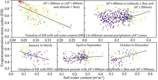
3.4. Correlation between ESI and SWC

Previous analyses has indicated a strong positive correlation between ET and WVP in different precipitation zones. Therefore, ET can directly monitor atmospheric water vapor condition. The relationship between ET and SWC is similar to that between ET and WVP, but the relationship is more complex than the latter and needs further discussion.

Figure 8 shows the correlation between ESI and SWC at monthly scales. A strong quadratic relationship exists between ESI and SWC, which is similar to the correlation between ET and SWC, especially in the alpine zones. The restriction of water supersaturation on ECR occurs with ease in the alpine zones. Given that the change in ESI with SWC is not a strictly monotone function in a large scale, the application of ESI in SWC monitoring needs to be studied in different zones.

As shown in Figure 9, a strong negative linear relationship exists between ESI and SWC in NM and SACOL stations, and R² = 0.47. The SWC is the main regulating factor of ET when the annual precipitation is lower than 400 mm, and ESI can represent the difference of SWC between the current underlying surface water condition and the fully humid condition to monitor the drought situation. When the annual precipitation exceeds 400 mm, the relationship between ESI and SWC is uncertain. As shown in Figure 9b, some of the scattered points of ESI and SWC show a positive correlation, whereas others show a negative correlation.

Figure 10a shows the time series of precipitation at the DHS, QYZ and XSBN stations with the annual precipitation exceeds 800 mm. The precipitation at these observation sites is mainly concentrated in the period from April to September. Before the occurrence of the main precipitation, that is, from January to March, SWC in these zones has relatively low level. At this time, as shown in Figure 10b, ESI is positively correlated to SWC. In the main precipitation period, the correlation between ESI and SWC is not clear due to the influence of precipitation on Rn and SWC, as shown in Figure 10c. After the occurrence of the main precipitation, that is, from October to December, the soil in these zones is basically in the state of water–supersaturated. The increase in temperature can be slowed down by water supersaturation. The ET process is inhibited, as shown in Figure 10d, and ESI is proportional to SWC. As shown in Figure 11, the relationship between ESI and SWC on the annual scale is similar to that on the monthly scale, but it is stronger than that on the monthly scale.

In summary, there exist significant differences in the changes in ET with SWC with different annual precipitations. The drought process is illustrated in Figure 12. Point B shows the state of SWC before the occurrence of the main precipitation in the humid areas. Point A indicates the water–supersaturated soil after the occurrence of the main precipitation in the humid zones. Point M indicates the early stage of drought, that is, the crop physiological process is unaffected by the decrease in SWC. Ta rises to the optimal temperature of crop physiological process with the occurrence of drought. Point C indicates that the drought process continues until the crop begins to die with water shortage. Point D indicates that with extreme drought, all crops die and SWC is almost zero. Then, in the humid areas, drought occurs, and the first B → M process occurs. Due to the decrease in SWC, the temperatures of air and crop are higher than usual, crop transpiration and soil evaporation increase correspondingly, and ET increases with the decrease in SWC. The drought continues, M → C occurs, crop is under water stress, and the transpiration is reduced. At the same time, the evaporation process of soil is limited with a water shortage, and ET decreases with SWC. In extreme drought, C → D can occur, and water is lacking at extreme levels. Transpiration decreases with the death of crops, the evaporation process is weak, ET decreases rapidly and tends to zero, and ET reaches zero even when the SWC is not zero.

The B → M → C → D process may occur in the humid areas, where the SWC is not always the main regulating factor of ET. However, in the water shortage areas, where the SWC is always the main regulating factor of ET, there may be only the M → C → D process; even in the zones with extremely low precipitation, the drought process may be directly C → D. Contrary to the drought process, such as the main precipitation process in the humid areas and the period after the main precipitation, the SWC is in the supersaturated state. The temperature is lower than usual due to water supersaturation, which inhibits the transpiration of crops and soil evaporation process and makes ET weaker than the normal state, that is, the process of B → A.

In the process of soil water supersaturation to extreme drought, ET and SWC have a typical quadratic relationship. However, from the analysis of observation data from the different zones, all sites are in the same period of rainfall and heat. In the period when the main precipitation occurs in the humid zone, the temperature increases with seasonal changes. The crop transpiration and soil evaporation increase due to the rise in environmental temperature. The cumulative effect of ET increasing caused by environmental factors and ET decreasing caused by the B → A process lead to the great uncertainty in ET change with SWC during the precipitation period in the humid area. As shown in Figure 10c, no significant correlation exists between ET and SWC in this period. After the main precipitation period, the SWC may be in the state of supersaturation, and the environmental temperature is also in the period of decreasing with seasonal change. A negative correlation exists between ET and SWC in this period because of the accumulation effect of environmental temperature and the B → A process, that is, ESI is proportional to SWC.

At the same time, due to the differences in crop water use efficiency, drought resistance, and soil characteristics, the locations of A, B, C, D, and M points are varied in different areas, which leads to the scattered points of ET and SWC not being closely and evenly distributed on both sides of the quadratic fitting line on a large scale.

3.5. Application of ET in Drought Monitoring

Research results in the literature [37] show that there exists a certain deviation between the GCOM–W1/AMSR–2 soil moisture product and the measured value, but the correlation between them is significant, which can represent the spatial difference characteristics of soil moisture on a large scale. In this study, the GCOM–W1/AMSR–2 soil volume water content was used in setting a threshold value in large-scale drought monitoring to simply distinguish different ET control areas to achieve the purpose of ESI in large-scale drought monitoring.

In the summer of 2022, severe high temperature and drought event occurred in southern China. As shown in Figure 13, the LST in Shanxi, Henan, Hebei, and Shandong in late June exceeded 60 °C, whereas that in the east of Sichuan and other southern areas exceeded 45 °C. By the middle of August, the high–temperature areas were concentrated in the east of Sichuan, Chongqing, Henan, Hubei, Hunan, Anhui, Jiangxi, Zhejiang, and Jiangsu; and the basically exceeded 45 °C. The continuous high temperature and little rainfall lead a lack of effective supplementation of soil moisture in these areas. As shown in Figure 14a, the soil moisture in the southern region from early June to late July was negative compared with that in the previous 10 days, indicating that the soil moisture in this region was in continuous deficit since early June. In the first 10 days of August, the soil moisture increased compared with the last 10 days of July, and in the middle of August, the soil moisture continued to show a deficit state. Figure 14b shows the difference between the mean value of soil moisture in July and August of 2013–2022 and the mean value of soil moisture in May, indicating the supplementation of summer precipitation to soil moisture each year. As shown in the figure, the soil water increment in the four summers of 2013, 2015, 2016, and 2022 was negative; thus, the soil water consumption in these summers is greater than soil water income, whereas the corresponding high temperature and drought events have occurred in southern China in these years. From the distribution of soil moisture increment in the summer, southern China was in a normal slightly wet state in 2021, so the difference between the parameters in 2022 and 2021 was used to represent the anomaly of soil moisture, as shown in Figure 14c. Except for the first 10 days of June and the middle 10 days of July, the soil moisture of the other 10 days in the summer of 2022 was lower than that of 2021, indicating that the summer of 2022 in southern China was drought–prone. Similarly, the LST in most regions of China in 2022 was higher than that in 2021. As shown in Figure 15a–c, the LST in August is evidently higher than that in 2021, and the deviation of some regions was about 20 °C. As southern China is a humid area, with the emergence of high temperatures in summer, ET in this area also increases, as shown in Figure 15d–f, which is a major feature of flash droughts.

The monitoring results of ESI are shown in Figure 16d–f. With the continuous high temperatures in the south and the reduction in soil moisture, ET increases and ESI decreases. In comparison with 2021, the deviations of ESI in most areas of southern China were negative. However, in the northern China, due to soil water deficit, ET decreases, ESI increases, and the deviations of ESI between 2022 and 2021 were positive. This finding is consistent with the relationship between ESI and SWC in different precipitation zones previously analyzed. To avoid the drought monitoring deviation caused by the regional difference of ESI, we use SWC as the standard to unify the ESI monitoring results in different regions. In this study, the areas with SWC ≥ 0.1 m³·m⁻³ and plateau areas (above 3 km in altitude) were simply defined as areas with a positive correlation between ESI and SWC, and the remaining areas were those with a negative correlation between ESI and SWC. Monitoring standards were formulated in different areas. The results are shown in Figure 16g–i. After regional monitoring, the drought in late June mainly occurred in Shaanxi, Gansu, Ningxia, Yunnan, eastern Sichuan, Chongqing, Hunan, Jiangxi, Fujian, and other parts of the country. By the end of July, the drought in the north was relieved, mainly in Longnan of Gansu. The drought situation in southern China was more serious in Hunan and Guangxi. By the middle of August, severe droughts were been detected in most southern regions, such as Sichuan, Chongqing, Henan, Hubei, Anhui, and Jiangxi. The monitoring results are similar to the regional distribution of soil moisture (Figure 16a–c), which can monitor the high temperatures and drought in most areas in the south. The simple zoning monitoring of ESI through soil moisture greatly improves the accuracy of large-scale drought monitoring.

4. Discussion

Generally, ET is regulated by heat and water. Radiation is the heat source of ET, and water is the controlling factor of ECR. Based on this study, from water supersaturation to water disappearance, ET has a quadratic correlation with SWC. However, for the differences in precipitation, crop species, and drought resistance, the characteristic curve and critical threshold of ET changing with SWC may significantly vary.

This study showed that the relationship between ET and WVP or that between ESI and SWC is not a single monotone function on a large scale. ET, as the water link of the soil–vegetation–atmosphere system, has always been a hot spot in related research fields. Similar research results to ours have been published. For example, Ying [38] and Wang [39] pointed out that there is a significant positive correlation between the soil water content and ET in arid barren and sandy lands on the basis of field observation data. Wang [40] also pointed out, through a farmland water experiment, that the soil water content is the main influencing factor of ET at the stage of wheat water shortage. At the same time, Liao [41] estimated the global ET through the global land surface temperature/vegetation coverage (LST/FVC) model. The results showed that the model with asynchronous ET and soil moisture change in semi–arid and semi–humid regions is better, and the model with synchronous ET and soil moisture change in humid regions is better, which also proves that the relationship between ET and soil moisture is different for precipitation.

Wang et al. [42] showed the changing relationship of relative evapotranspiration (LE/PET) with leaf area index (LAI) and relative soil water content (RSWC) during the entire growth period of winter wheat through the long–term observation data of the Yucheng experimental station, as shown in Figure 17. Based on the Yucheng experimental data, the change in LE/PET with RSWC and LAI during the entire growth period of wheat was shown. It was pointed out that, when the LAI of wheat is less than the critical value, the ET is mainly determined by the surface soil water content. When the LAI is greater than the critical value, if the soil water is insufficient, the soil water content is still the control factor of ET. When soil water is sufficient, LAI is the controlling factor of LE/PET. As shown in Figure 17, before April 2, the RSWC decreased. However, as the temperature increased, the LE/PET increased. After the first irrigation, the RSWC increased rapidly. Later, with the growth of vegetation, the RSWC consumption and the LAI increased, and the LE/PET decreased. After the second irrigation in the filling period, the LAI began to decline. While the soil moisture content decreased, the LE/PET also decreased. To sum up, in the early stage of vegetation growth, i.e., when the LAI is small, the LE/PET is inversely proportional to RSWC. When the water is sufficient, the vegetation status and RSWC become the main influencing factors of LE/PET. After the filling period, the LAI decreases, and the water does not effectively increase vegetation transpiration. As the RSWC decreases, the LE/PET also decreases. This result is similar to the conclusions obtained in this paper, as shown in Figure 10.

Similar to our research, Yue et al. [43] analyzed the measured data of the SACOL station in a semi–arid area and pointed out that, in semi–arid areas, the relationship between relative evapotranspiration and soil water content is exponential, as shown in Figure 18.

It has been shown that the relationship between relative evapotranspiration and soil water is different under different water, heat and vegetation conditions. The relationship between ESI(1–ET/PET) and soil water is also different under different water, heat, and vegetation conditions. However, in large-scale drought monitoring, it will inevitably span different precipitation zones and different vegetation underlying surfaces. The differences in soil hydrothermal characteristics and vegetation drought resistance undoubtedly increase the difficulty in drought monitoring. At present, the effective way to improve the accuracy of large-scale drought monitoring is to formulate criteria considering different areas and periods, combining climate regionalization, underlying surface type, and digital elevation information. To achieve successful large-scale drought monitoring, remote sensing is an effective way with unique advantages. Although the accuracy of monitoring can be improved by formulating drought monitoring criteria in different zones and periods, how to use remote sensing data to accurately estimate ET is also a major difficulty for ESI to use in large-scale drought monitoring [22,23].

In addition, as shown in Figure 12, some points in the process of ET changing with SWC have great significance. For example, M is the optimal temperature and water combination point for crop physiological state. If SWC is lower than this threshold, then the crop is subject to water stress, or even yield reduction, thereby threatening food security. Determining the temperature and water threshold at this point is conducive to crop disaster prediction. Point C is the location where crops begin to die, which is the critical threshold for some physiological processes of crops to appear irreversible, which is greatly significant for predicting crop death caused by drought and assessing the influence of climate change [44].

The analysis in this study indicated that water and heat are two key factors affecting ET, and different water and heat regulation mechanisms will correspond to different monitoring standards of ESI. If ESI is used to accurately monitor large-scale drought, a refined zoning of the study area should be conducted, and monitoring standards and drought classification standards in different regions should be developed. This paper only used SWC for simple zoning to achieve the ESI monitoring of drought on a large scale, but in actual zoning, precipitation, temperature, altitude, and the underlying surface type should also be considered. The establishment of the refined zoning scheme of the monitoring area is the basis for accurate ESI monitoring.

5. Conclusions

In this study, on the basis of observation data, an empirical model for retrieving land surface evapotranspiration from FY–4A satellite remote sensing was established, and the regulation of water and heat factors on ET was analyzed in different precipitation zones using nine stations in different precipitation areas and different underlying surfaces. The variation characteristics of ET during the drought period and the applicability of ESI in different areas were discussed. The main conclusions are as follows.

(1) The correlation analysis of ET with Rn, Ta, WVP, and SWC in different precipitation regions shows that there is a linear relationship between ET, Rn, Ta and WVP in different regions, but the slopes of the fitting line between ET and parameters are different due to the precipitation. The ECR has a quadratic relationship with WVP and SWC. When WVP = 0.182 kPa and SWC = 0.217 m³∙m⁻³, ECR reaches the maximum level.

(2) In extreme water shortage areas, water is always the decisive factor of ET regulation. ET and ECR show strong positive linear correlations with SWC, and the Rn has an effect on ET only when the water content of the earth–atmosphere system reaches a certain level. In areas with sufficient water, Rn, as a heat source, is the main regulating factor of ET. ECR changes slightly with WVP and SWC. Moreover, a weak negative correlation is shown between ECR and WVP and SWC, which indicates that water condition is not the main regulating factor of ECR in areas with sufficient water. When the annual precipitation between 200 mm and 800 mm, water and Rn participate in the regulation of ET. The relationships between WVP and ET and ECR exhibit a strong positive correlation, and the relationships between SWC and ET and ECR are more complex, showing quadratic relationships.

(3) Based on the data of six observation stations in the Heihe River basin, an empirical model for land surface ET retrieving using NDVI, average land surface temperature and land surface temperature difference was established using the artificial intelligence particle swarm optimization algorithm, and the remote sensing retrieval of large-scale ET based on geostationary satellites remote sensing data was achieved. The correlation coefficient R² between the ET estimated by the empirical model and the measured value was 0.48; a certain deviation exists in the value, with the root mean square error being 24 W·m⁻². On the basis of ET retrieval products, combined with the relationship between ESI and SWC previously analyzed, the ESI results are divided by SWC, and monitoring standards were formulated in different regions to improve the accuracy of large-scale drought monitoring. It turns out to be the case that using AMSR–2 soil volume water content to simply distinguish different control areas of ET can achieve the remote sensing monitoring of large-scale drought. The accuracy of ESI in monitoring drought on a large scale can be improved by formulating monitoring standards in different regions.

References

1. Xu, G. Part 4: Drought Disasters and Drought Mitigation. J. Arid. Meteorol. 1990, 4, 34–43. [Google Scholar]
2. WMO. Early Warning Systems for Drought Preparedness and Drought Management. In Proceedings of the Expert Group Meeting, Lisbon, Portugal, 5–7 September 2000; pp. 1–8. [Google Scholar]
3. Sivakumar, M.; Stefanski, R.; Bazza, M.; Zalaya, S.; Wilhite, D.; Magalhaes, A. High Level Meeting on National Drought Policy: Summary and Major Outcomes. Weather Clim. Extrem. 2014, 3, 126–132. [Google Scholar] [CrossRef] [Green Version]
4. Yang, X. Research and Application of Meteorological Drought Monitoring Indexes in Northwest China. Meteorol. Mon. 2007, 33, 90–96. [Google Scholar]
5. Hao, X.; Zhang, Q.; Yang, Z.; Wang, X.; Yue, P.; Han, T.; Wang, S. A new method for drought monitoring based on land surface energy balance and its preliminary application to the Hedong region of Gansu province. Chin. J. Geophys. 2016, 59, 3188–3201. [Google Scholar]
6. Li, Y.; Zhang, L.; Zhang, H.; Pu, Z. Drought Monitoring Based on CABLE Land Surface Model and Its Effect Examination of Typical Drought Events. Plateau Meteorol. 2015, 34, 1005–1018. [Google Scholar]
7. Kogan, F. Development of Global Drought Watch System Using NOAA/AVHRR Data. Adv. Space Res. 1993, 13, 219–222. [Google Scholar] [CrossRef]
8. Kogan, F. Application of Vegetation Index and Brightness Temperature for Drought Detection. Adv. Space Res. 1995, 15, 91–100. [Google Scholar] [CrossRef]
9. Jackson, R.; Slaler, P.; Pinter, P. Discrimination of Growth and Water Stress in Wheat by Various Vegetation Indices Through Clear and Turbid Atmosphere. Remote Sens. Environ. 1983, 13, 187–208. [Google Scholar] [CrossRef]
10. Sandhoh, I.; Rasmussen, K.; Andersen, J. A simple Interpretation of the Surface Temperature-Vegetation Index Space for Assessment of Surface Moisture Status. Remote Sens. Environ. 2002, 79, 213–224. [Google Scholar] [CrossRef]
11. Carlson, T.; Gillies, R.; Perry, E. A Method to Make Use of Thermal Infrared Temperature and NDVI Measurement to Infer Soil Water Content and Fractional Vegetation Cover. Remote Sens. Rev. 1994, 52, 45–59. [Google Scholar] [CrossRef]
12. Sun, L.; Wang, F.; Wu, J. Drought Monitoring by Remote Sensing in Winter-Wheat-Growing Area of China. Trans. Chin. Soc. Agric. Eng. 2010, 1, 243–249. [Google Scholar]
13. Watson, K.; Rowen, L.; Offield, T. Application of Thermal Modeling in the Geologic Interpretation of IR Image. Remote Sens. Environ. 1971, 3, 2017–2041. [Google Scholar]
14. Jackson, R.; Idso, S.; Reginato, R. Canopy Temperature as A Crop Water Stress Indicator. Water Resour. Res. 1981, 17, 1133–1138. [Google Scholar] [CrossRef]
15. Moran, M.; Clarke, T.; Inoue, Y.; Vodal, A. Estimating Crop Water Deficit Using the Relation between Surface Air Temperature and Spectral Vegetation Index. Remote Sens. Environ. 1994, 49, 246–263. [Google Scholar] [CrossRef]
16. Shao, X.; Yao, F.; Zhang, J.; Li, H. Analysis of Drought in North China Based on Evapotranspiration Drought Index. Meteorol. Mon. 2013, 39, 1154–1162. [Google Scholar]
17. Zhang, X.; Li, J.; Qin, Q.; Han, Y.; Guan, J. Comparison and Application of Several Drought Monitoring Models in Ningxia, China. Trans. Chin. Soc. Agric. Eng. 2009, 25, 18–23. [Google Scholar]
18. Shan, Y.; Gong, A.; Su, Y.; Liu, W.; Jiang, W. Improvement of Soil Moisture Monitoring Using EVI as A Key Parameter Based on TVDI in the North China Plain. In Proceedings of the 2013 IEEE International Geoscience and Remote Sensing Symposium—IGARSS, Melbourne, VIC, Australia, 21–26 July 2013; IEEE: Piscataway Township, NJ, USA, 2014; pp. 3738–3741. [Google Scholar]
19. Guo, N.; Wang, X. Advances and Developing Opportunities in Remote Sensing of Drought. J. Arid. Meteorol. 2015, 33, 1–18. [Google Scholar]
20. Zhang, D.; Meng, L.; Qu, J.; Zhang, W.; Wang, L. Estimation of Surface Soil Moisture in Cornfields Using A Modified MODIS-Based Index and Considering Corn Growth Stages. IEEE J. Sel. Top. Appl. Earth Obs. Remote Sens. 2017, 10, 5618–5631. [Google Scholar] [CrossRef]
21. Guo, N.; Wang, W.; Wang, X.; Hu, D.; Wang, L. Agricultural Drought Remote Sensing Monitoring and Analysis Platform in Northwest China Base on FY-3 Data. In Proceedings of the 2019 International Conference on Meteorology Observations (ICMO), Chengdu, China, 28–31 December 2019. [Google Scholar] [CrossRef]
22. Liu, S.; Huang, Z.; Liu, L. Numerical Simulation of the Evapotranspiration Process in the Soil-Vegetation-Atmosphere Continuum. Acta Geogr. Sin. 1996, 51, 118–126. [Google Scholar]
23. Wang, J.; Liu, S.; Sun, M.; Guo, N.; Bastiaanssen, W. Monitoring ET with Remote Sensing and the Management of Water Resource on A Basin Scale. J. Arid. Meteorol. 2005, 23, 1–7. [Google Scholar]
24. Anderson, M.; Kustas, W. Thermal Remote Sensing of Drought and Evapotranspiration. Eos Trans. Am. Geophys. Union 2013, 89, 233–234. [Google Scholar] [CrossRef]
25. Meng, X.; Lü, S. Estimation of Land Surface Heat Flux in the Heterogeneous Underlying Surface in Jinta Oasis Based on RemoteSensing and Numerical Model. Plateau Meteorol. 2012, 31, 910–919. [Google Scholar]
26. Yang, F.; Zhang, Q.; Hunt, J.E.; Zhou, J.; Sha, S.; Li, Y.; Yang, Z.; Wang, X. Biophysical Regulation of Evapotranspiration in Semiarid Croplands. J. Soil Water Conserv. May 2019, 74, 309–318. [Google Scholar] [CrossRef]
27. Yu, G.; Yanbin, H.; Yanfen, W. 2003–2005 China Flux Observation (ChinaFLUX) Carbon and Water Flux Observation Dataset; Science Data Bank: Beijing, China, 2018. [Google Scholar]
28. Wang, K.; Liang, S. An Improved Method for Estimating Global Evapotranspiration Based on Satellite Determination of Surface Net Radiation, Vegetation Index, Temperature, and Soil Moisture. J. Hydrometeor. 2008, 9, 712–727. [Google Scholar] [CrossRef]
29. Yang, Q.; Wu, J.; Li, Y.; Li, W.; Wang, L.; Yang, Y. Using the Particle Swarm Optimization Algorithm to Calibrate the Parameters Relating to the Turbulent Flux in the Surface Layer in the Source Region of the Yellow River. Agric. For. Meteorol. 2017, 232, 606–622. [Google Scholar] [CrossRef] [Green Version]
30. Becker, F.; Li, Z.L. Towards a Local Split-Window Method over Land Surfaces. Int. J. Remote Sens. 1990, 11, 369–393. [Google Scholar] [CrossRef]
31. Wang, L.; Guo, N.; Wang, W.; Zuo, H. Optimization of the Local Split-Window Algorithm for FY-4A Land Surface Temperature Retrieval. Remote Sens. 2019, 11, 2016. [Google Scholar] [CrossRef] [Green Version]
32. Wang, L.; Zuo, H.; Wang, W. A Simple Method for Surface Radiation Estimating Using FY-4A Data. J. Appl. Meteorol. Climatol. 2021, 60, 763–777. [Google Scholar] [CrossRef]
33. Priestley, C.; Taylor, R. On the Assessment of Surface Heat Flux and Evaporation using Large-scale Parameters. Mon. Weather Rev. 1972, 100, 81–92. [Google Scholar] [CrossRef]
34. Jiang, L.; Islam, S. Estimation of Surface Evaporation Map over Southern Great Plains Using Remote Sensing Data. Water Resour. Res. 2001, 37, 329–340. [Google Scholar] [CrossRef] [Green Version]
35. Yang, K.; Huang, G.; Tamai, N. A Hybrid Model for Estimating Global Solar Radiation. Sol. Energy 2001, 70, 13–22. [Google Scholar] [CrossRef]
36. Haque, A. Estimating actual areal evapotranspiration from potential evapotranspiration using physical models based on complementary relationships and meteorological data. Bull. Eng. Geol. Environ. 2003, 62, 57–63. [Google Scholar] [CrossRef]
37. Wang, S.; Jaing, L.; Wang, J. Retrieval of Soil Moisture Based on Multi-frequency Microwave Remote Sensing: Study of HiWATER. Remote Sens. Technol. Appl. 2020, 35, 1414–1425. [Google Scholar]
38. Ying, G.; Hou, Y.; Zhang, Y.; Xue, Y.; Wang, H.; Tian, Y.; Si, Q. Responses of Evapotranspiration of Dominant Plants to Soil Moisture in Desert Steppe. Anim. Husb. Feed Sci. 2016, 37, 18–22. [Google Scholar]
39. Wang, X.; Zhang, L.; Liu, L.; Huang, Z.; Liu, X. Numerical Calculation of the Relationship between Evapotranspiration and Soil Moisture in Arid Sandy Region. J. Desert Res. 1996, 16, 388–391. [Google Scholar]
40. Wang, H.; Liu, C. Evapotranspiration, Soil Evaporation and Water Efficiet Use. Acta Geogr. Sin. 1997, 52, 447–454. [Google Scholar]
41. Liao, Q. Study on Remote Sensing Inversion of Surface Evapotranspiration. Master’s Thesis, Guilin University of Technology, Guangxi, China, 2020. [Google Scholar]
42. Wang, J.; Li, X.; Liu, E.; Yu, Q. The Relationship between Relative Evapotranspiration and Leaf Area Index and Surface Soil Water Content in Winter Wheat Field of North China Plain. Chin. J. Eco-Agric. 2003, 11, 32–43. [Google Scholar]
43. Yue, P.; Zhang, Q.; Zhang, L.; Yang, Y.; Wang, W.; Yang, Z.; Li, H.; Wang, S.; Sun, X. Biometeorological effects on carbon dioxide and water-use efficiency within a semiarid grassland in the Chinese Loess Plateau. J. Hydrol. 2020, 590, 125520. [Google Scholar] [CrossRef]
44. Choat, B.; Brodribb, T.; Brodersen, C.; Duursma, R.; Lopez, R.; Medlyn, B. Triggers of Tree Mortality under Drought. Nature 2018, 558, 531–539. [Google Scholar] [CrossRef]
Figure 1. Location of observation sites. The red triangle represents the ground stations, the green font represents the name of the station used to develop the ET retrieval model, and the blue font represents the name of the station used to analyze ET regulation.
Remotesensing 14 06190 g001
Figure 2. Valid data filtering, in which the red dotted line is used to distinguish the data between stations. In the lower abscissa, the interval between two scales is one year.
Remotesensing 14 06190 g002
Figure 3. Correlation analysis of the ET to Rn ratio (ET/Rn) and normalized difference vegetation index (NDVI) (a), mean land surface temperature (LSTm) (b), and the range of LST difference (DLSTR) (c).
Remotesensing 14 06190 g003
Figure 4. Comparison between ET estimated by Equation (2) and the measured value of the station in Table 1, where the bold black line represents the fitting line of scattered points and the dotted black line represents the 1:1 line.
Remotesensing 14 06190 g004
Figure 5. Time series of the different parameters in all observation sites in Table 2, in which the red dotted line distinguish the data between stations and in the lower abscissa, the interval between two scales is one year. Among them, (a) includes the monthly changes in Ta and rainfall; (b) includes the monthly changes in SWC and WVP; (c) includes the monthly changes in Rn, Hs, and LE; and (d) includes the monthly cumulative rainfall and TE calculated by Equation (1).
Remotesensing 14 06190 g005aRemotesensing 14 06190 g005b
Figure 6. Correlation between ET and Rn (a), Ta (b), WVP (c), and SWC (d). The black dots are the data of the alpine zones. The red fitting line indicates the data of SQH station. The green fitting line indicates the alpine zones, except the SQH station. The yellow fitting line indicates the area where the altitude is less than 3 km, with annual precipitation levels lower than 800 mm (as NM, SACOL and CBS stations in this study). The purple fitting line indicates the area with an altitude of lower than 3 km and annual precipitation exceeding 800 mm (as DHS, QYZ, and XSBN stations in this study). Figure 7 and Figure 8 are similar to Figure 6.
Remotesensing 14 06190 g006
Figure 7. Correlation between ET conversion rate (ECR = LE/Rn) and WVP (a) and SWC (b). The black fitting line represents the result of all points. Figure 8, Figure 9, Figure 10 and Figure 11 are similar to Figure 7.
Remotesensing 14 06190 g007
Figure 8. Variation of ESI with SWC. (a) is the data of all sites in Table 2 and (b) is the data of the alpine zones.
Remotesensing 14 06190 g008
Figure 9. Variation of ESI with SWC in different precipitation zones. (a) is the data of SQH, NM and SACOL stations with the annual precipitation is lower than 400 mm, and the blue line is the fitting line of the scattered points and (b) is the data of other stations. Additionally, the orange line is the fitting line of the scattered points. Figure 11 is similar to Figure 9.
Remotesensing 14 06190 g009
Figure 10. Variation of ESI with SWC in different periods at the DHS, QYZ and XSBN stations with the annual precipitation exceeds 800 mm. (a) is the time series of average precipitation of the DHS, QYZ and XSBN stations; (b) is the correlation between ESI and SWC from January to March; (c) is the correlation between ESI and SWC from April to September; and (d) is the correlation between ESI and SWC from October to December.
Remotesensing 14 06190 g010
Figure 11. Variation of ESI with SWC at an annual scale. (a) is the data of all sites and (b) is the data of the alpine zones. The blue fitting line indicates the data of NM and SACOL stations, the orange fitting line indicates the data of other stations, and the black fitting line indicates the data of all stations.
Remotesensing 14 06190 g011
Figure 12. Schematic of ET changing with SWC.
Remotesensing 14 06190 g012
Figure 13. Distributions of LST and ET in the summer of 2022, where (ac) are the distributions of LST in late June, late July, and middle August, respectively, and (df) are the distributions of ET in late June, late July, and middle August, respectively.
Remotesensing 14 06190 g013
Figure 14. Soil moisture increment, where (a) shows the increase in soil moisture in each 10–day period in the summer of 2022, that is, the difference between the current 10–day period and the previous 10–day period; (b) shows the difference between the average soil volume water content from July to August and that in May of that year; and (c) shows the moisture difference between each 10–day period in the summer of 2022 and the corresponding 10 days in 2021.
Remotesensing 14 06190 g014
Figure 15. Comparison of LST and ET in 2022 with those in 2021, where (ac) are the distributions of the LST difference in late June, late July, and middle August, respectively, and (df) are the distributions of the ET difference in late June, late July, and middle August, respectively.
Remotesensing 14 06190 g015
Figure 16. Distributions of soil moisture difference between 2002 and 2021 and ESI monitoring results, where (ac) are the distributions of soil moisture difference in late June, late July, and middle August, respectively; and (df) are the normal ESI monitoring results in late June, late July, and middle August, respectively; and (gi) are the monitoring results of ESI after zoning based on soil moisture.
Remotesensing 14 06190 g016
Figure 17. The variations of relative evapotranspiration (LE/PET) with leaf area index (LAI) and relative soil water content (RSWC) in the surface layer of winter wheat from turn–green to harvest (cited from the literature [42]).
Remotesensing 14 06190 g017
Figure 18. Relationship between the daily ET/PET SWC at 5 cm depth during the growing seasons from 2007 to 2012 (cited from the literature [43]).
Remotesensing 14 06190 g018