Article

Radiative Transfer Image Simulation Using L-System Modeled Strawberry Canopies

1
Gulf Coast Research and Education Center, School of Forest Fisheries, and Geomatics Sciences, University of Florida, Plant City, FL 33563, USA
2
Gulf Coast Research and Education Center, Department of Horticultural Sciences, University of Florida, Plant City, FL 33563, USA
3
School of Forest Fisheries, and Geomatics Sciences, University of Florida, Plant City, FL 33563, USA
4
Centre d’Etudes Spatiales de la BIOsphère—UPS, CNES, CNRS, IRD, Université de Toulouse, 31401 Toulouse, France
*
Author to whom correspondence should be addressed.
Remote Sens. 2022, 14(3), 548; https://doi.org/10.3390/rs14030548
Submission received: 4 December 2021 / Revised: 20 January 2022 / Accepted: 21 January 2022 / Published: 24 January 2022
(This article belongs to the Special Issue Advances in Remote Sensing for Crop Monitoring and Yield Estimation)

Abstract

:
The image-based modeling and simulation of plant growth have numerous and diverse applications. In this study, we used image-based and manual field measurements to develop and validate a methodology to simulate strawberry (Fragaria × ananassa Duch.) plant canopies throughout the Florida strawberry growing season. The simulated plants were used to create a synthetic image using radiative transfer modeling. Observed canopy properties were incorporated into an L-system simulator, and a series of strawberry canopies corresponding to specific weekly observation dates were created. The simulated canopies were compared visually with actual plant images and quantitatively with in-situ leaf area throughout the strawberry season. A simple regression model with L-system-derived and in-situ total leaf areas had an A d j   R 2 value of 0.78. The L-system simulated canopies were used to derive information needed for image simulation, such as leaf area and leaf angle distribution. Spectral and plant canopy information were used to create synthetic high spatial resolution multispectral images using the Discrete Anisotropic Radiative Transfer (DART) software. Vegetation spectral indices were extracted from the simulated image and used to develop multiple regression models of in-situ biophysical parameters (leaf area and dry biomass), achieving A d j   R 2 values of 0.63 and 0.50, respectively. The Normalized Difference Vegetation Index (NDVI) and the Red Edge Simple Ratio (SRre) vegetation indices, which utilize the red, red edge, and near infrared bands of the spectrum, were identified as statistically significant variables (p < 0.10). This study showed that both geometric (canopy seize metrics) and spectral variables were successful in modeling in-situ biomass and leaf area. Combining the geometric and spectral variables, however, only slightly improved the prediction model. These results show the feasibility of simulating strawberry canopies and images with inherent geometrical, topological, and spectral properties of real strawberry plants. The simulated canopies and images can be used in applications beyond creating realistic computer graphics for quantitative applications requiring the depiction of vegetation biological processes, such as stress modeling and remote sensing mission planning.

Graphical Abstract

1. Introduction

Advances in plant measurement techniques have made it possible to construct a geometric model of a specific plant from structural parameters [1,2]. The construction of such models to simulate plants for computer graphics has long been a field of active study [3,4]. Simulated plants have very promising applications, not only for modeling complex biological processes [5], but also for enriching training datasets for deep learning applications [6].
Plant growth simulation can be modeled as a dynamic system with dynamic structures [7], in which not only the values of the state variables but also the set of state variables change over time. Several modeling techniques have been developed over the years, among which is the Lindenmayer-system (L-system) [8]. The L-system made it possible to model dynamically reconfigurable plant structures. With the mathematical theory of plant development [8] and the ability to incorporate geometric interpretations [9], the L-system has been used in various agricultural research applications. Benoit et al. (2014) [10] employed an L-system-based root model to generate images of simulated roots. Ubbens et al. (2018) used L-system-generated leaf images to augment a dataset to help train a neural network system [6]. Rokhana et al. (2020) used the L-system as a polynomial function to simulate and visualize the growth of soybean (Glycine max L. Merrill) plants in response to various combinations of fertilizers [11]. Xin et al. (2020) used a stochastic L-system to achieve 3D reconstruction of grape fruit clusters (Vitis vinifera L. cv. Merlot) [12].
Several studies have utilized image-based positional information for plant modeling [13,14]. Structure from Motion (SfM) [15] analysis was used to generate point clouds from plant images [16,17,18], which were then used to acquire leaf segment and petiole silhouettes. Laser scanning has been used to derive positional information from scanned point clouds [16,19]. A combination of image information, including image-based point clouds and in-situ measurements of leaves and petioles, was used to extract canopy size metrics, which were subsequently used to model canopy leaf area and biomass [20,21]. This method can provide essential geometrical information needed to model crops, including strawberry (Fragaria × ananassa Duch.), throughout the entire growing season.
Strawberry is a high-value fruit crop grown worldwide. However, strawberry production requires intensive management, as plants and fruit are highly sensitive to various biotic and abiotic factors [22]. Remote sensing data, captured with the right configuration and at the right time, combined with advanced analysis techniques [23], can be used to assist strawberry farm management. Understanding canopy structure characteristics is key to many strawberry farming applications as well as preventative and management actions. Models described in Guan et al. and Abd-Elrahman et al. [20,21] have focused on developing empirical models of the relationship between plant biophysical parameters and remote sensing information. These models, however, do not attempt to integrate radiative transfer interactions inside the canopy structure to quantify photosynthesis and plant growth and to plan remote sensing data acquisition mission parameters such as image spectral, spatial, and temporal resolutions.
Physical Radiative Transfer (RT) models can simulate the propagation of radiation in Earth landscapes and the atmosphere and can therefore simulate remote sensing images of these landscapes using physically described mechanisms [24]. Ideally, they consider all possible observation configurations with any sun and sensor viewing directions. The amount of energy received at each pixel in an image can vary significantly due to image formation geometry, expressed by the variations in energy source, object, and sensor geometry [25], which can be expressed using RT models [26]. Methods to derive canopy structure characteristics using physical RT models through inversion procedures [27,28,29,30] and forward procedures [31,32] have been used. Precisely simulated images based on RT modeling have a great potential in many domains, including agriculture and forestry. For example, they can be simulated for various vegetation stress conditions and growth stages. They can constitute synthetic training data for deep learning models. They can also be used to prepare observation campaigns and design future satellite missions through the determination of optimal spectral bands and time of satellite overpass, given the geometry and optical properties of the studied land surfaces. However, these approaches require canopy structure characteristics that are difficult to acquire and are often obtained from generic pre-existing databases. Plants simulated using actual biological characteristics are key to the accurate RT image simulation of vegetation canopies.
This study aims to demonstrate and validate (1) the use of in-situ measurements in strawberry plant growth simulation models and (2) the utilization of the simulated plants in RT-based synthetic image simulation. In-situ measurements and image-derived information of strawberry plants are used to provide geometric, structural, and phenological characteristics to inform growth functions. The simulated plants are validated against canopy size metrics of existing strawberry plants throughout the growing season. A physical RT model is calibrated using simulated canopy information to create synthetic multispectral images of strawberry canopies at different growth stages. Spectral vegetation indices derived from the simulated image are used to assess the simulation results. This research is an important step towards realizing a biologically driven simulation that goes beyond graphical representation and towards emerging applications such as the visualization of crop model outputs, facilitating training datasets for deep learning, and planning remote sensing missions.

2. Methods

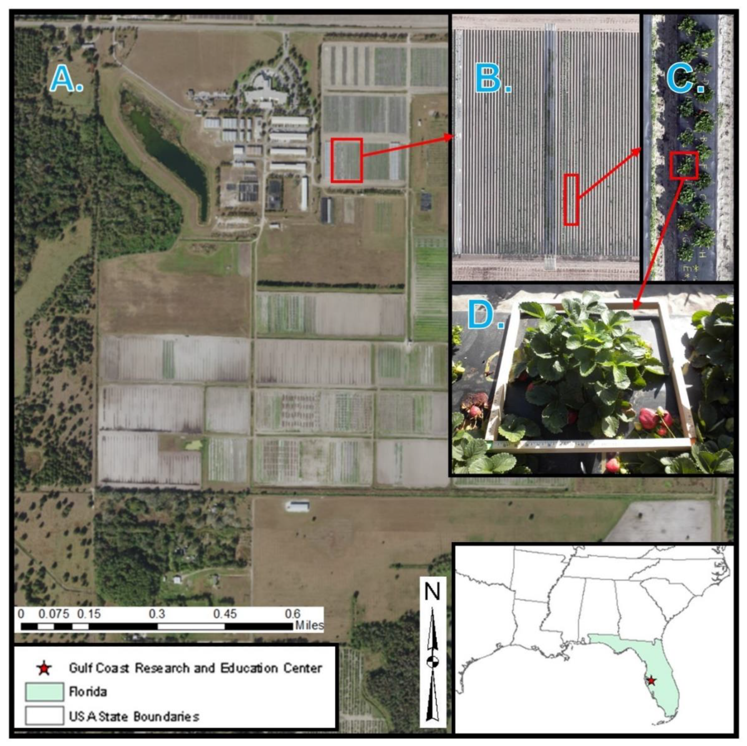
2.1. Study Site and Data Collection

The University of Florida’s Gulf Coast Research and Education Center (GCREC) experimental farm in Wimauma, FL (27°45′40″N, 82°13′40″W) (Figure 1A) served as the study site. Sweet Sensation® “Florida127” strawberry plants were planted on a raised bed (Figure 1B–D) and maintained according to the commercial growing standards in Central Florida. “Florida127” is one of the major strawberry cultivars grown in Florida, United States. Two representative plants were used to provide information for plant simulation.
High spatial resolution close-range images were captured using a hand-held Nikon COOLPix S630 at approximately 60 cm from the plant canopy from more than 24 angles covering the whole plant (Figure 2). A wood frame was positioned around the canopy for model scaling. The length of the petioles (leaf petioles) and size of the leaves were manually measured every 4–5 days from 17 October to 17 December to study growth patterns.
Spectral reflectance and transmittance data of the leaves, needed for the RT image simulation (with wavelengths ranging from 400 nanometers to 2400 nanometers), were acquired using a FieldSpec4 Spectroradiometer leaf clip (Figure A1A). The reflectance data of the plastic bed and soil were acquired using a FieldSpec4 Spectroradiometer pistol grip (Figure A1B). These were performed on 34 canopies every other week during the 2017/2018 season, concurrent with the image data collection. During each acquisition, the spectral measurements of a mature (dark green, expanded to nearly full size, and more fibrous) leaflet and a young (light green, still expanding, and small enough to barely cover the collecting area of the FieldSpec 4 device) leaflet from each canopy were collected.
Mobile ground-based images and in-situ leaf area and dry biomass acquired every week during the 2017/2018 strawberry season (Figure A2A) were used for the quantitative assessment of the growth models and RT simulated images. Details about how this dataset was collected and the methods used to derive the canopy size metrics (planimetry area, average canopy height, and standard deviation of canopy height) from the captured images are presented in Guan et al. and Abd-Elrahman et al. [20,21].

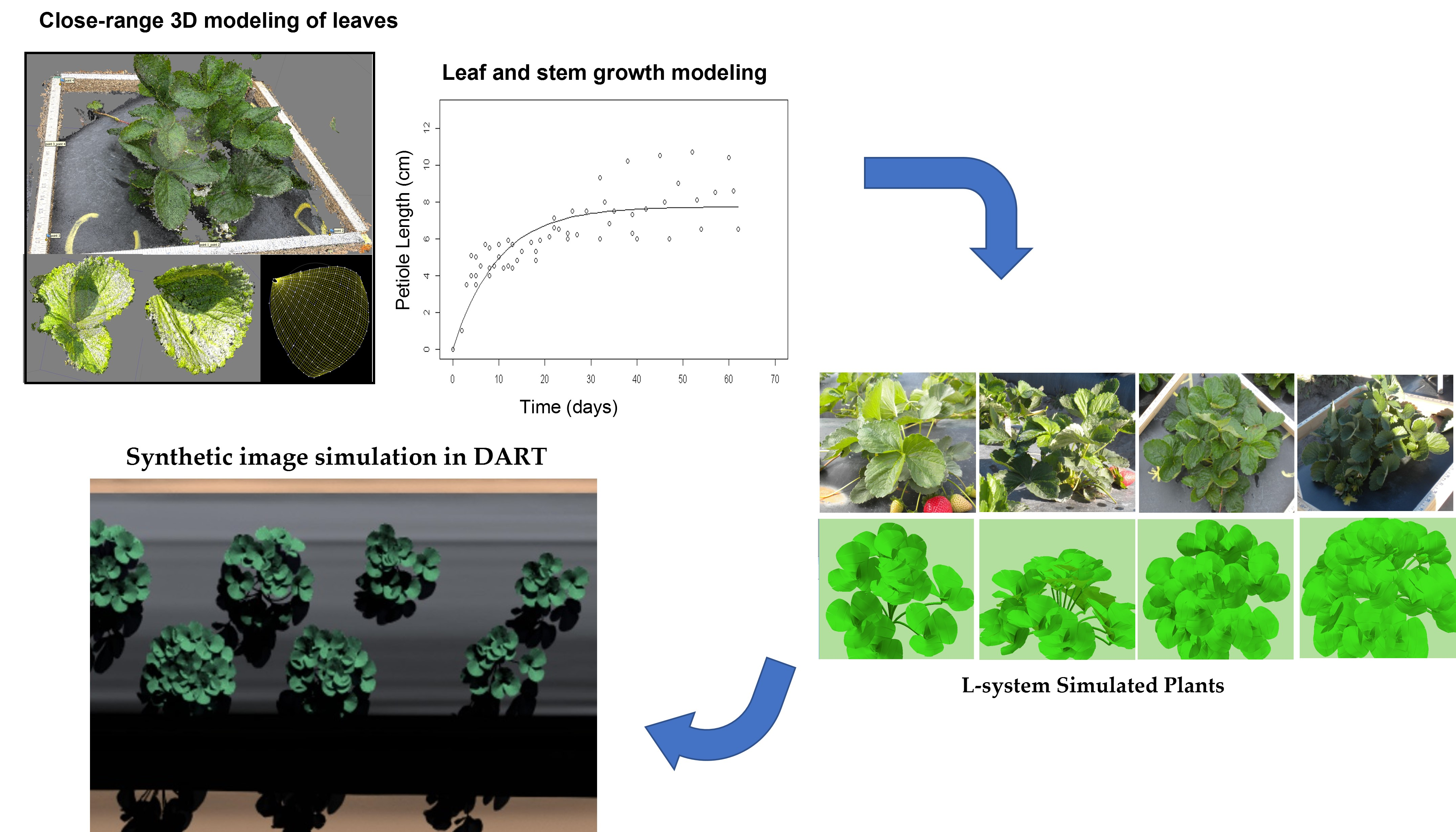
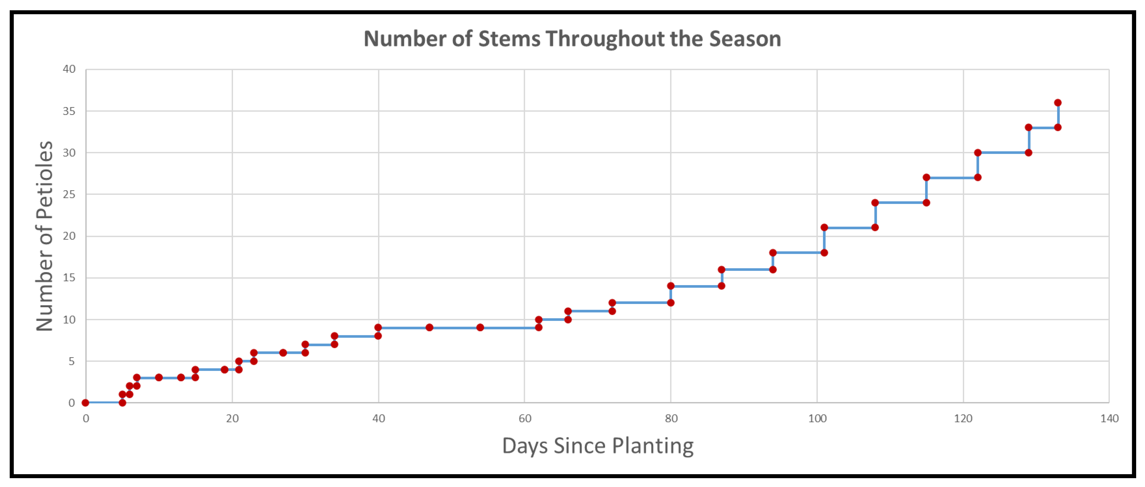
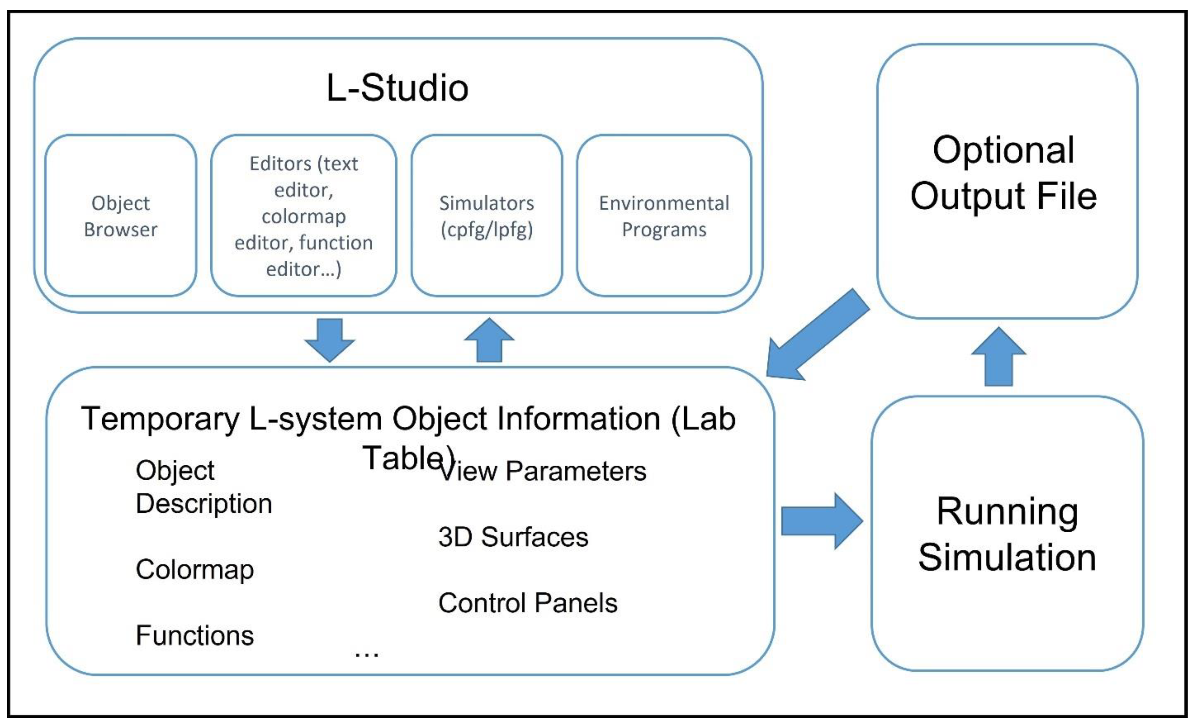
2.2. Simulation of Plant Growth Using L-System

This study focused on the “Florida127” strawberry to simulate its plant growth throughout the growing season using the L-system assisted by field measurement. Figure 3 shows the workflow used to generate the L-system strawberry model and results assessment. A global-to-local approach was adopted to model the strawberry canopy, starting with the silhouette of the whole canopy and moving to leaf and petiole details. Data required to model plant growth were obtained from high-resolution images, leaf and petiole size field measurements, and topological observations (e.g., number and frequency of emerging petioles). Dynamic strawberry growth models were then created and simulated throughout the strawberry growing season. The simulated canopies were analyzed weekly within the growth cycle to match mobile ground-based image and in-situ biomass and leaf area data collections. Canopy sizes from simulated and actual plants were compared to determine the suitability of simulations to model in-situ leaf area and biomass.
Simulation language and L-Studio environment: Plant growth simulations in this study were conducted using L-Studio [33,34] software (Figure A2). An L-system model in the L-studio environment consists of two components: (i) a generative algorithm in a generator modeling language called a plant and fractal generator with a continuous parameter (cpfg/lpfg) [35] and (ii) a set of graphically defined entities. The cpfg/lpfg is a language constructed based on rewriting rules that capture the development of plant components over time. In general, rewriting is a technique for defining complex objects by successively replacing parts of simple initial objects. The graphically defined entities were defined and manipulated using editors (function, curve, and surface) within the L-studio environment.
Modeling individual leaves: The information needed to model individual leaves was extracted from the close-range hand-held images acquired for “Florida127” strawberry plants throughout the growing season. The images were processed using a self-calibrating bundle adjustment [36] implemented in the Agisoft Metashape software (version 1.4.0.5650) [37] (Figure 2). The tie-points needed for the bundle adjustment were detected automatically by identifying local features within each image, which were then matched across multiple images using the Structure from Motion (SfM) technique [15]. Figure 4A shows a dense point cloud of one of the observed strawberry canopies with leaf-level details. Figure 4B,C shows a dense point cloud of one of the leaves. A 2.4 mm-resolution Digital Surface Model (DSM) representing the shape of the leaf was created using the Agisoft software.
The DSM was analyzed using The ESRI’s ArcMap software v10.5. Since the surface editor of L-studio uses 16 × 16 point grid to create a Bézier surface to reconstruct the shape of the leaf, a 16 × 16 matrix of sample points was positioned on the DSM to acquire 3D information at these locations (Figure 5A) through the ArcMap’s software geospatial analysis tools. This 16 × 16 matrix of sample points was input into L-Studio. A comparison of the L-system surface and a point cloud of a leaf from different angles is shown in Figure 5B–D.
Stem angle modeling: To describe the shape and gesture of a petiole (leaf petiole), two angles (angles α   and   β in Figure 6) need to be defined. As the plant grows, new petioles develop from the crown (basal part of the plant) and push the existing petioles outward due to the petiole orientation and space competition. As a result, the existing petioles gradually deviate from an imaginary vertical line at the center. This phenomenon is described by a gradual change of angle α (Figure 6). As the petioles develop and mature, the increasing mass of the petioles and the leaves attached to their ends bend the petioles down to the bed surface. Meanwhile, due to the phototropism phenomenon [38,39], the petioles grow upward to maximize the exposure of leaves to sunlight. These two tendencies result in angle β changes during growth. We measured the angle α on captured images and observed a change from zero as the petiole emerges to 29 degrees on average at the end of the season (134 days from the first petiole emergence). Similarly, we observed that angle β changes from zero to 19 degrees on average when the petiole reaches maturity (i.e., it reaches its maximal length about 50 days from petiole emergence).
Growth function modeling: The L-system is designed as a dynamic structure [8] with a prominent feature of modeling canopy growth as a phenomenon. The model can represent the dynamic change of both the topology and geometry of the canopies throughout their growth cycle. The weekly high-resolution images captured throughout the strawberry season were used to extract time-stamped measurements of leaf length and width, petiole length and angle, and leaf curvature angles. The observed petiole number, petiole length, and leaf length were used to model the canopy growth function.
The change in petiole number shows the dynamic nature of strawberry plant topology and drives leaf area accumulation. The number of petioles was counted (Figure 7) and utilized in the cpfg [35] coding as explained in the next section. The changes in petiole and leaf lengths exhibit the dynamic nature of the plants as a geometric aspect. Measuring petiole lengths from the point clouds extracted from the image SfM analysis results was difficult due to the small size of the petioles as well as plant occlusion. Alternatively, petiole dimensions were measured using a ruler. Figure 8A shows how petiole lengths change with time, and Figure 8B shows the petioles after lining up all the petiole observations according to their corresponding age(different colors represent different petioles).
An asymptotic regression model is presented in Equation (1) to depict a limited growth of sigmoidal elongation of segments such as the petioles or leaves [9]:
L = a ( 1 e bt )
where L is the dimension of the leaves or petioles, t is the time expressed in days after planting, and a and b are coefficients to be determined by regression fitting of the observed in-situ leaf and petiole measurements. Figure 8C shows petiole dimension data fitted against the asymptotic model. Petiole and leaf dimensions were then predicted on a daily interval and normalized to accommodate the function editor requirements in L-s. Studio, which has x and y axes ranging from 0 to 1 (Figure 8D). Figure A3 shows the generated petiole and leaf growth functions through the L-studio function editor.
L-system cpfg coding: The cpfg code used in this study was developed to set up the rewriting rule guiding plant development in both plant topology and geometry. This code first described how the petioles emerge and occupy the space and how this behavior affects the silhouette of the canopy. Then, the details of each petiole, such as the change of petiole length, orientation, and the growth of leaves, were modeled.
A root node was initiated in the model with a certain number of petioles attached to it, and each petiole was given a dormant/delay time. The numbers of petioles changing over time and dormant/delay time were determined by the in-situ measurements. The pattern of how the petioles spread in the azimuth direction was assumed to be symmetrical in all directions. The pattern of how petioles occupy the zenith dimensions was guided by observations of how the petiole angles change over time.
Every petiole was modeled as a composition of more detailed components (i.e., several segments representing the petiole part and a trifoliate leaf attached to the top), defined as a decomposition process in cpfg. The angles between the segments allow the petiole to bend during their elongation, and the elongation was guided by the developed growth function. A similar approach was adopted to generate the leaves. In practice, the normalized growth function of leaf length and leaf width is nearly the same [40,41,42], so the growth function of leaf length was chosen to control changes in leaf dimensions. A stochastic effect was applied to the size of the leaves and length of the petioles according to the mean and standard deviation of leaf and petiole field measurements.
Model validation: A scale factor was calculated using modeled leaf dimensions and in-situ measurements. The L-system models were scaled to the real strawberry canopy dimensions using this scale factor before conducting model validation. Two types of L-system model validations were conducted. The first validation was conducted by comparing the plant leaf area output from the L-system simulation with the average in-situ total leaf area of two plants of “Florida127” measured weekly by destructive methods [20,21]. Plants simulated by the L-system were exported as 3D models. A computer program was developed in Python to compute the total canopy leaf area from the extracted 3D canopy models.
The second validation assessed the L-system model capacity to develop a leaf area regression model to predict leaf area using canopy size metrics (i.e., canopy area, canopy average height, and standard deviation of canopy height). We hypothesized that if the leaf area statistical prediction model was validated, the L-system model could depict the real plant to some degree. The simulated 3D models were transformed into a 3D point cloud and processed into a DSM by sampling the point cloud into a grid while recording only the maximum elevation. This process was conducted via the Quick Terrain Modeler V1.2 software (2015) to estimate canopy size parameters.

2.3. Radiative Transfer Image Simulation

In this study, images were simulated using the Discrete Anisotropic Radiative Transfer (DART) model [24], which computes radiation propagation through the whole Earth–atmosphere system in the entire optical domain from the visible to thermal infrared parts of the electromagnetic spectrum [43,44]. Leaf, canopy, bed, and soil optical, geometrical, and/or structural properties were input into the DART model to simulate a “scene” (3D structures with geometric and spectral properties). Scene elements can be represented as volumes of turbid medium and/or facets. The date and time of the data simulation and the geolocation of the study site were used to calculate the solar angle. Radiation propagation was simulated with a discrete ordinate method (i.e., rays can propagate only along a finite number of directions). A single DART simulation provides images for a number of predefined viewing directions and spectral bands. These images were processed and analyzed to create a set of vegetation spectral indices. Regression analysis was then carried out using the vegetation indices and canopy size parameters to model the total leaf area and biomass of the canopies. A detailed description of these steps is explained in the following subsections.
Geometric and spectral configuration: Recreating the lighting geometry, which is the angle of the object–sensor with respect to that of the object–sun, is crucial in RT-based image simulation. The date and time of the data simulation and the geolocation of the study site were used to calculate the solar angle [45].The imaging sensor was assumed to be mounted on a mobile mapping platform collecting nadir-looking images. The imaging sensor in the simulation was assumed to have five bands (blue, green, red, near infrared, and red edge) mimicking the spectral properties of the widely used MicaSense multispectral camera (Table 1).
Image simulation: Three scene objects were included in the simulation: soils, plastic beds, and strawberry canopies. The soils and the plastic beds were treated as surface media with complex geometry. The elevations created using image information were imported into the DART software to guarantee the faithfulness of the representation of the geometric complexity of the soil and plastic bed objects. The spectral properties of the soil and plastic elements were input as spectral reflectance over a certain range of the spectrum acquired by the FieldSpec4 spectroradiometer using the device shown in Figure A1B.
In this study, the canopies were treated as turbid media [46]. Therefore, foliar elements (leaves and petioles) were randomly distributed. Under this assumption, canopies could be described by addressing two components: (i) the spectral properties of the foliar elements and (ii) the canopy structure formed by the distribution of these elements. The spectral properties of the canopy leaves were described as reflectance and transmittance over the specific range of wavelengths acquired by the FieldSpec4 spectroradiometer using the device shown in Figure A1A. The structure of the canopy is described by the spatial distribution of the leaf-area volume density, which is defined as the total one-sided leaf area of photosynthetic tissue per unit canopy volume. Integrating it over the canopy height gives the leaf area index (LAI), which is the one-sided leaf area per unit horizontal ground surface area [47]. Canopy structure is also described by the leaf normal orientation distribution function, which is another expression of the leaf area distribution (LAD) [48]. A total of 14 “Florida127” strawberry canopies simulated using the L-system, representing different data collection points throughout the season, were imported into the DART software to provide the canopy structural elements. The L-system-simulated canopies allowed the modeling of the geometry and inner structure of the canopies, which were used to compute the LAI and LAD. Radiation propagation interactions with the created scene elements were then computed to create the synthetic image. During the modeled energy–object interaction, radiation is scattered multiple times before being received by the hypothetical imaging sensor. Images containing the reflectance of five bands adopting the spectral properties of the MicaSense Red Edge camera were created. A true color (RGB: red, green, and blue) visualization of the image was created using the DART simulation model.
Extraction of spectral indices: ESRI’s ArcMap software v10.5 was used to process the simulated images and to delineate individual canopy boundaries. The reflectance values of the five bands for all pixels within each canopy were extracted, and the average values within the individual canopies were calculated (Table 2). Six vegetation indices were computed as the spectral transformation of two or more band reflectances for each canopy [49]. Table 3 shows a description of the vegetation indices used in this study.
Simulated image validation: Multiple regression analysis was performed using R-studio software version 1.1.453 [56]. In the developed models, only the significant variables at the 90% confidence level that were not highly correlated (Variance Inflation Factor (VIF) [57] less than 10) were kept in the models. Three dependent variables were used to assess the performance of the simulated images and compare the performance with other plant canopy data sources: (1) leaf area of the L-system simulated plants; (2) in-situ leaf area, and (3) in-situ biomass. Four sets of independent variables were used to model each of the three dependent variables: (a) canopy size metrics (canopy area, average height as a baseline, and standard deviation of height) extracted from mobile ground-based images [20,21], (b) canopy size metrics extracted from the L-system simulated canopies, (c) vegetation indices extracted from the DART-simulated images, and (d) a combination of L-system canopy size metrics and vegetation indices.
In this analysis, we attempted to evaluate the suitability of using the DART-simulated spectral data to model canopy biophysical parameters and compare these results to corresponding models utilizing geometric canopy information. The analysis identified the statistically significant indices and their simulated bands. We also assessed the use of a combination of the canopy size metrics extracted from the L-system canopies and the canopy spectral indices extracted from the DART-simulated images to model the canopy leaf area and dry biomass.

3. Results

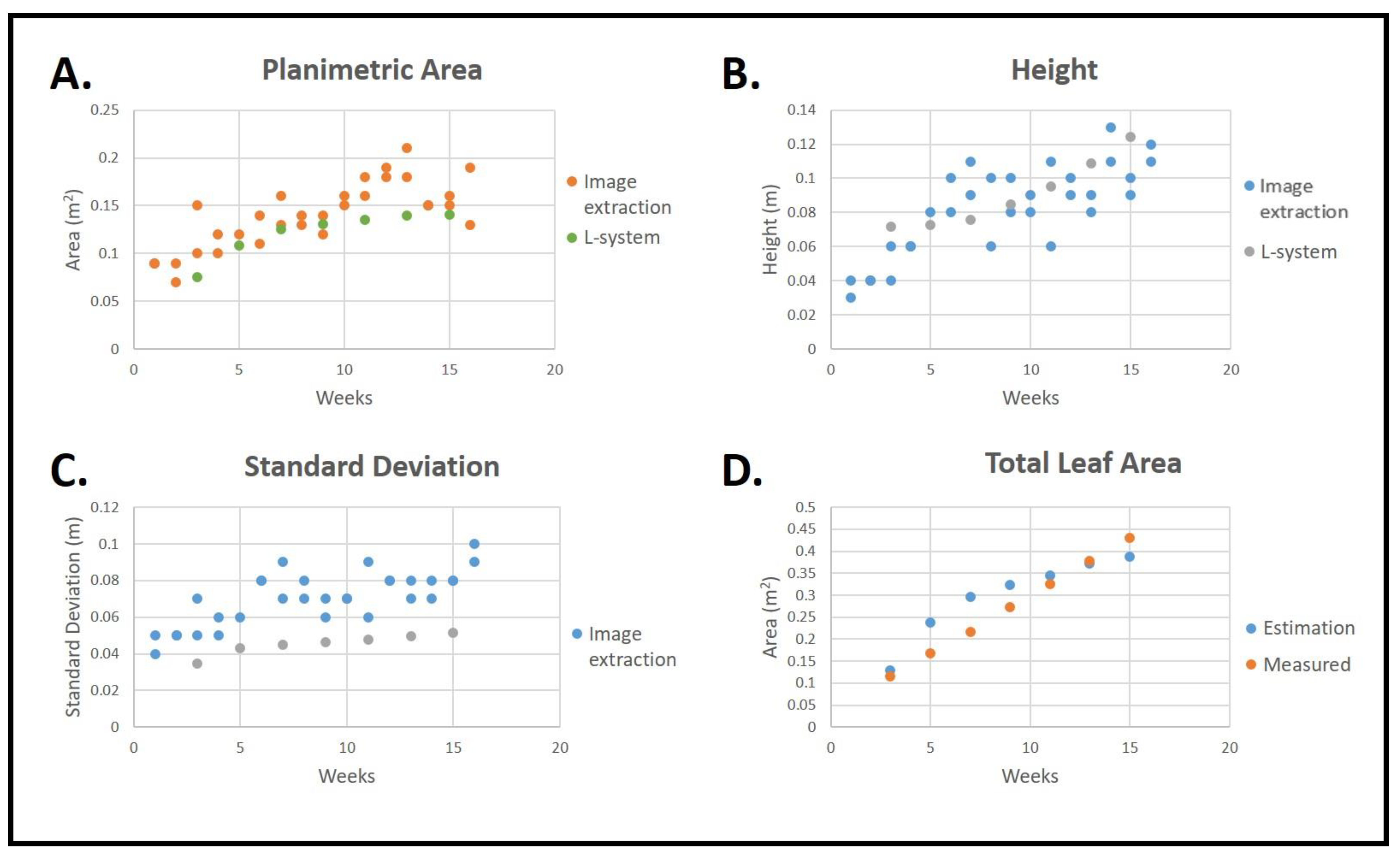
3.1. L-System Canopy Growth Simulation Results

In-situ observation of strawberry plant growth showed that a single petiole takes up to 50 days to reach its maturity (maximum length), after which the size of both petiole and leaf remains approximately the same, assuming the plant was not subject to stress (e.g., drought, pests, and diseases). Table 4 shows the summary statistics of petiole length and leaf size at maturity. The mean and standard deviation of the petiole length and leaf size serve the purpose of adding a stochastic effect to the L-system model, assuming that the maturity length and size of the petioles and leaves follow a normal distribution (leaf size: 0.074 ± 0.12   m ; petiole length: 0.093 ± 0.184   m ), as shown in Table 4.
Equations (2) and (3) show the asymptotic growth models of petiole length and leaf length of “Florida127” (Figure A3). Petiole and leaf lengths were generated at daily intervals using these equations and normalized to values between 0 and 1 for input into the L-system function editor. The normalized leaf length was chosen to depict leaf size growth. The custom L-system code developed to simulate the strawberry canopies was executed through the L-studio software simulator, and canopies corresponding to the weekly collected in-situ data and mobile image acquisitions were produced. Figure 9 shows a visual comparison between real canopies and L-system models at their corresponding growth age.
P e t i o l e   L e n g t h = 7.73 ( 1 e 0.10 t )  
L e a f   L e n g t h = 5.73 ( 1 e 0.18 t )  
Model performance was assessed quantitatively by comparing the total leaf area of the L-system simulated plants with in-situ plant leaf area measured at the corresponding growth age (Figure 10), showing A d j   R 2 = 0.78 of the simple regression model relating the simulated and in-situ leaf areas. Differences between each of the three canopy size metrics extracted from the L-system simulation and corresponding canopy metrics extracted from the mobile images throughout the season were also used to evaluate the L-system model results as shown in Figure 11A–D.

3.2. Radiative Transfer Image Simulation Results

The simulated canopy images (Figure 12) were validated against in-situ leaf area and dry biomass measurements conducted throughout the growing season as well as the leaf area of the canopies simulated using the L-system. We used 16 plants simulated to match 16 episodes of in-situ image acquisition over the strawberry growing season (Table 2). Figure 13 represents the adjusted R2 values (R2 values after accounting for the number of independent variables) of the tested models. The multiple linear regression analysis of the L-system simulated leaf area, in-situ leaf area, and in-situ biomass as dependent variables and the vegetation indices listed in Table 3 as independent variables (Equations (4)–(6)) resulted in A d j   R 2 values of 0.58, 0.63, and 0.51, respectively. The NDVI and SRre vegetation indices were identified as statistically significant variables (p < 0.10).
L e a f   A r e a L s y s = 1.55 + 1.0316 N D V I + 0.4110 S R r e  
L e a f   A r e a i n s i t u = 1.67 + 1.3122 N D V I + 0.3472 S R r e
D r y   B i o m a s s i n s i t u = 252.85 + 170.38 N D V I + 59 S R r e
The highest A d j   R 2 of the models utilizing vegetation indices was achieved for the in-situ leaf area, which contradicted our expectations of having higher A d j   R 2 for the leaf areas computed from the L-system simulated canopies since the DART simulation is derived directly from the L-system canopies.
Combining the L-system canopy size metrics with the spectral variables resulted in a slight increase in the A d j   R 2 values for the in-situ leaf area and dry biomass (0.68 and 0.58) compared to using the spectral indices only (0.62 and 0.51). This may suggest that both the spectral and geometrical canopy data can be used independently to model canopy leaf area and biomass and still obtain close results. In the meantime, combining the two datasets could also have the potential to explain additional variability in the leaf area and biomass variables.
The A d j   R 2 of the in-situ leaf area and biomass models using simulated data (L-system canopy size metrics or spectral data) are significantly lower than those obtained when using the canopy metrics extracted from the mobile images, which is expected due to the direct correspondence between the in-situ leaf area and dry biomass measurements and the image-based canopy size metrics. Although this could be attributed to the expected shortcomings of all simulation methods, it also raises the potential for improving the simulation results.
An A d j   R 2 value of 0.87 was obtained when the L-system canopy size metrics were used as independent variables to model the leaf area of the same L-system simulated canopies. This lower-than-expected value highlights the limitation of using canopy metrics (canopy area, average canopy height, and standard deviation of canopy height) to explain canopy leaf area variability as well as other limitations in the statistical model (multiple linear regression) that was used.

4. Discussion

This study used close-range images, field measurements, and spectral measurements to build an L-system dynamic strawberry growth model and simulate RT images of strawberry plants throughout the growing season. In-situ measurements and information extracted from images were used to quantitatively evaluate the L-system and RT simulation results. Our results highlight the ability of L-system models to predict leaf area and size metrics of the strawberry canopy and suggest the feasibility of using simulated plants in agricultural applications. For example, physical radiative transfer modeling using accurate structure and geometry characteristics can be used to produce simulated aerial images that characterize biological processes such as strawberry disease stresses or genotypes.
Images and field measurements provided topological and geometric information that enabled plant simulation throughout the season. This information guided the whole structure of the L-system cpfg code development. While close-range image analysis was a valuable source for some aspects of the simulation, such as leaf surface modeling, the in-situ measurements provided more accurate, fine-scale geometric information, such as petiole and leaf lengths, as well as the topological information needed to control the growth function. Simulated plants at different growth levels were validated, and the data used for model development (e.g., leaf and petiole dimensions, images, and point clouds) were different from the data used in the validation process (e.g., in-situ total leaf area).
The standard deviation of height of the simulated canopies, among all the canopy size metric parameters, had the least correspondence to validation data (standard deviation of canopy heights extracted from mobile images). Because this metric reflects canopy internal structure, it could indicate a limitation in our L-system model when dealing with canopy structure details such as where new petioles emerge and how they compete for space and solar radiation with existing petioles. This limitation could also be due to the fact that both the close-range imagery (used in model development) and the mobile imagery (used in model results validation) did not acquire enough information on the inside parts of the canopy to enable descriptions of canopy structure. More in-situ observations or the use of high-density laser scanning techniques could address this limitation.
Although only one cultivar (Florida127) of strawberry was simulated in this study, the code developed in the study could be modified and used to simulate other cultivars and other crops that have similar growth habits with minor adjustments. Incorporating crop yield, common management practices, such as pruning, other canopy elements such as flowers and fruits, as well as other physiological and environmental processes, such as stress effects from water and nutrition deficiencies, weather conditions, diseases, and pests, could expand the use of this model in agricultural management applications. This can be achieved by adding features to the simulation code as well as using situational L-systems to deal with disease and pest effects. Such sophisticated modeling serves as a solid foundation for image simulation in physical radiative modeling.
Unlike most image and plant simulation studies, we attempted to develop simulated images using datasets that have high resemblance to reality, benefiting from the L-system models. One of the most important parameters needed for a radiative transfer image simulation (e.g., using DART) is the estimation of the canopy geometrical aspects. The L-system’s ability to simulate plant canopies and our attempts to assist the simulation with field measurements and observations facilitated faithful representation and computation of the geometrical and structural canopy properties extracted from the simulated canopies.
Having a moderate goodness of fit for the in-situ leaf area and dry biomass models signals the possibility of using simulated images to experiment with imaging parameters that can be used to predict in-situ strawberry biophysical parameters (leaf area and dry biomass in our case). This indicates, however, that there is room to improve the simulation models. For example, in this study, we only used in-situ measurement from a small number of plants (e.g., one plant to observe petiole emergence along the season), and we have not incorporated other plant elements, such as strawberry flowers and fruits. Enriching the datasets and adding more features to the L-system models can improve their faithfulness and capacity to depict more biological processes.
This study results emphasize the importance of specific spectral bands and canopy size metrics for modeling leaf area, as they highlight the importance of using sensors with red, red edge, and near infrared bands to develop canopy leaf area and biomass prediction models. This again represents a simple example of the potential of using canopy and image simulation in applications such as image planning. The faithful simulation of canopies and images can be used to identify the best bands, flying height (image resolution), and acquisition time for specific applications such as diagnosing the effect of specific plant stressors. Images of plants subject to different types of stressors, such as pests, diseases, drought, and nutrient deficiencies, could be simulated by modifying the L-system and DART simulation parameters to accommodate the geometrical and spectral changes at the leaf and canopy levels.
Through this procedure, a series of images can be simulated to present canopies under diverse stressors and management practices using different spectral (e.g., band wavelengths and widths) configurations, image spatial resolutions, sun–sensor–object geometries, and field topographies and configurations. Analyzing these images could aid in identifying the best parameters, configurations, and analysis techniques for numerous applications such as detecting and diagnosing different stressor types. The simulated images could also be used to enrich training data for automated object detection and image classification using machine and deep learning techniques, reducing the need for costly image acquisition efforts. They may also be used in inversion models to estimate plant biophysical parameters from actual images. More research is needed to overcome some of the limitations of this study by incorporating more in-situ observations, modeling different strawberry varieties, and integrating different physiological and phenological plant behaviors along the growth cycle.

5. Conclusions

This study used close-range images, field measurements, and spectral measurements to build an L-system dynamic strawberry growth model and simulate RT images of strawberry plants throughout the growing season. In-situ measurements and information extracted from images were used to quantitatively evaluate the L-system and RT simulation results.
Our results highlight the ability of L-system models to predict leaf area and size metrics of the strawberry canopy and suggest the feasibility of using simulated plants in agricultural applications. The Normalized Difference Vegetation Index (NDVI) and the Red Edge Simple Ratio (SRre) vegetation indices extracted from simulated images were identified as statistically significant variables. This study showed that both geometric (canopy seize metrics) and spectral variables were successful in modeling in-situ biomass and leaf area. The simulated canopies and images have the potential to be used in applications beyond creating realistic computer graphics or synthetic representations for quantitative applications requiring the depiction of vegetation biological processes.

Author Contributions

Conceptualization, A.A.-E. and Z.G.; Data curation, Z.G.; Formal analysis, Z.G.; Methodology, A.A.-E.; Project administration, A.A.-E.; Software, J.-P.G.-E.; Supervision, S.A.; Validation, V.W.; Visualization, B.W.; Writing—original draft, Z.G.; Writing—review and editing, A.A.-E., V.W., S.A., B.W., J.-P.G.-E. and B.D. All authors have read and agreed to the published version of the manuscript.

Funding

This research received no external funding.

Conflicts of Interest

The authors declare no conflict of interest.

Appendix A

Figure A1. Using the Fieldspec4 Spectroradiometer to measure (A) leaf spectra using the leaf clip, and (B) soil and plastic bed spectra using the pistol grip.
Remotesensing 14 00548 g0a1
Figure A2. Growth function in L-studio editor. (A) Growth function of a petiole. (B) Growth function of a leaf.
Remotesensing 14 00548 g0a2
Figure A3. L-studio framework and components.
Remotesensing 14 00548 g0a3

References

  1. Gibbs, J.A.; Pound, M.; French, A.P.; Wells, D.M.; Murchie, E.; Pridmore, T. Approaches to three-dimensional reconstruction of plant shoot topology and geometry. Funct. Plant Biol. 2017, 44, 62–75. [Google Scholar] [CrossRef] [PubMed] [Green Version]
  2. Yan, G.; Jiang, H.; Luo, J.; Mu, X.; Li, F.; Qi, J.; Hu, R.; Xie, D.; Zhou, G. Quantitative Evaluation of Leaf Inclination Angle Distribution on Leaf Area Index Retrieval of Coniferous Canopies. J. Remote Sens. 2021, 2021, 2708904. [Google Scholar] [CrossRef]
  3. Gauthier, M.; Barillot, R.; Schneider, A.; Chambon, C.; Fournier, C.; Pradal, C.; Robert, C.; Andrieu, B. A functional structural model of grass development based on metabolic regulation and coordination rules. J. Exp. Bot. 2020, 71, 5454–5468. [Google Scholar] [CrossRef] [PubMed]
  4. Wang, H.; Cimen, E.; Singh, N.; Buckler, E. Deep learning for plant genomics and crop improvement. Curr. Opin. Plant Biol. 2020, 54, 34–41. [Google Scholar] [CrossRef] [PubMed]
  5. Auzmendi, I.; Hanan, J.S. Investigating tree and fruit growth through functional–structural modelling: Implications of carbon autonomy at different scales. Ann. Bot. 2020, 126, 775–788. [Google Scholar] [CrossRef] [PubMed]
  6. Ubbens, J.; Cieslak, M.; Prusinkiewicz, P.; Stavness, I. The use of plant models in deep learning: An application to leaf counting in rosette plants. Plant Methods 2018, 14, 6. [Google Scholar] [CrossRef] [Green Version]
  7. Giavitto, J.-L.; Michel, O. MGS: A Programming Language for the Transformations of Topological Collections; Technical Report 61-2001; LaMI–Université d’Évry Val d’Essonne: Évry, France, 2011. [Google Scholar]
  8. Lindenmayer, A. Mathematical models for cellular interactions in development I. Filaments with one-sided inputs. J. Theor. Biol. 1968, 18, 280–299. [Google Scholar] [CrossRef]
  9. Prusinkiewicz, P.; Lindenmayer, A. The Algorithmic Beauty of Plants; Springer Science & Business Media: Berlin/Heidelberg, Germany, 2012. [Google Scholar]
  10. Benoit, L.; Rousseau, D.; Belin, É.; Demilly, D.; Chapeau-Blondeau, F. Simulation of image acquisition in machine vision dedicated to seedling elongation to validate image processing root segmentation algorithms. Comput. Electron. Agr. 2014, 104, 84–92. [Google Scholar] [CrossRef] [Green Version]
  11. Rokhana, R.; Herulambang, W.; Indraswari, R. Machine Learning and Polynomial–L System Algorithm for Modeling and Simulation of Glycine Max (L) Merrill Growth. In Proceedings of the 2020 International Electronics Symposium (IES), Surabaya, Indonesia, 29–30 September 2020; pp. 463–467. [Google Scholar]
  12. Xin, B.; Liu, S.; Whitty, M. Three-dimensional reconstruction of Vitis vinifera (L.) cvs Pinot Noir and Merlot grape bunch frameworks using a restricted reconstruction grammar based on the stochastic L-system. Aust. J. Grape Wine Res. 2020, 26, 207–219. [Google Scholar] [CrossRef]
  13. Neubert, B.; Franken, T.; Deussen, O. Approximate image-based tree-modeling using particle flows. ACM Trans. Graph. 2007, 26, 88. [Google Scholar] [CrossRef]
  14. Okabe, M.; Owada, S.; Igarash, T. Interactive Design of Botanical Trees using Freehand Sketches and Example-based Editing. Comput. Graph. Forum 2005, 24, 487–496. [Google Scholar] [CrossRef]
  15. Westoby, M.; Brasington, J.; Glasser, N.; Hambrey, M.; Reynolds, J. ‘Structure-from-Motion’ photogrammetry: A low-cost, effective tool for geoscience applications. Geomorphology 2012, 179, 300–314. [Google Scholar] [CrossRef] [Green Version]
  16. Livny, Y.; Yan, F.; Olson, M.; Chen, B.; Zhang, H.; El-Sana, J. Automatic reconstruction of tree skeletal structures from point clouds. In Proceedings of the ACM SIGGRAPH Asia 2010 papers, Seoul, South Korea, 15 December 2010; pp. 1–8. [Google Scholar]
  17. Quan, L.; Tan, P.; Zeng, G.; Yuan, L.; Wang, J.; Kang, S.B. Image-based plant modeling. ACM Trans. Graph. 2006, 25, 599–604. [Google Scholar] [CrossRef]
  18. Tan, P.; Zeng, G.; Wang, J.; Kang, S.B.; Quan, L. Image-based tree modeling. ACM Trans. Graph. 2007, 26, 87. [Google Scholar] [CrossRef]
  19. Xu, H.; Gossett, N.; Chen, B. Knowledge and heuristic-based modeling of laser-scanned trees. ACM Trans. Graph. 2007, 26, 19. [Google Scholar] [CrossRef]
  20. Abd-Elrahman, A.; Guan, Z.; Dalid, C.; Whitaker, V.; Britt, K.; Wilkinson, B.; Gonzalez, A. Automated Canopy Delineation and Size Metrics Extraction for Strawberry Dry Weight Modeling Using Raster Analysis of High-Resolution Imagery. Remote Sens. 2020, 12, 3632. [Google Scholar] [CrossRef]
  21. Guan, Z.; Abd-Elrahman, A.; Fan, Z.; Whitaker, V.M.; Wilkinson, B. Modeling strawberry biomass and leaf area using object-based analysis of high-resolution images. Isprs J. Photogramm 2020, 163, 171–186. [Google Scholar] [CrossRef]
  22. Saridas, M.A.; Simsek, O.; Donmez, D.; Kacar, Y.A.; Kargi, S.P. Genetic diversity and fruit characteristics of new superior hybrid strawberry (Fragaria× ananassa Duchesne ex Rozier) genotypes. Genet. Resour. Crop Evol. 2021, 68, 741–758. [Google Scholar] [CrossRef]
  23. Zheng, C.; Abd-Elrahman, A.; Whitaker, V. Remote Sensing and Machine Learning in Crop Phenotyping and Management, with an Emphasis on Applications in Strawberry Farming. Remote Sens. 2021, 13, 531. [Google Scholar] [CrossRef]
  24. Gastellu-Etchegorry, J.-P.; Yin, T.; Lauret, N.; Cajgfinger, T.; Gregoire, T.; Grau, E.; Feret, J.-B.; Lopes, M.; Guilleux, J.; Dedieu, G.; et al. Discrete Anisotropic Radiative Transfer (DART 5) for Modeling Airborne and Satellite Spectroradiometer and LIDAR Acquisitions of Natural and Urban Landscapes. Remote Sens. 2015, 7, 1667–1701. [Google Scholar] [CrossRef] [Green Version]
  25. Aber, J.S.; Marzolff, I.; Ries, J.B. Chapter 10—Image Interpretation. In Small-Format Aerial Photography; Aber, J.S., Marzolff, I., Ries, J.B., Eds.; Elsevier: Amsterdam, The Netherlands, 2010; pp. 139–157. [Google Scholar]
  26. Nicodemus, F.E.; Richmond, J.C.; Hsia, J.J.; Ginsberg, I.W.; Limperis, T. Geometrical considerations and nomenclature for reflectance. In Radiometry; Jones and Bartlett Publishers, Inc.: Burlington, MA, USA, 1992; pp. 94–145. [Google Scholar]
  27. Banskota, A.; Serbin, S.P.; Wynne, R.H.; Thomas, V.A.; Falkowski, M.J.; Kayastha, N.; Gastellu-Etchegorry, J.P.; Townsend, P.A. An LUT-Based Inversion of DART Model to Estimate Forest LAI from Hyperspectral Data. IEEE J. Sel. Top. Appl. Earth Obs. Remote Sens. 2015, 8, 3147–3160. [Google Scholar] [CrossRef]
  28. Gastellu-Etchegorry, J.P.; Gascon, F.; Estève, P. An interpolation procedure for generalizing a look-up table inversion method. Remote Sens. Env. 2003, 87, 55–71. [Google Scholar] [CrossRef]
  29. Kimes, D.; Gastellu-Etchegorry, J.; Estève, P. Recovery of forest canopy characteristics through inversion of a complex 3D model. Remote Sens. Env. 2002, 79, 320–328. [Google Scholar] [CrossRef]
  30. Yáñez-Rausell, L.; Malenovský, Z.; Rautiainen, M.; Clevers, J.G.P.W.; Lukeš, P.; Hanuš, J.; Schaepman, M.E. Estimation of Spruce Needle-Leaf Chlorophyll Content Based on DART and PARAS Canopy Reflectance Models. IEEE J. Sel. Top. Appl. Earth Obs. Remote Sens. 2015, 8, 1534–1544. [Google Scholar] [CrossRef] [Green Version]
  31. Couturier, S.; Gastellu-Etchegorry, J.-P.; Patiño, P.; Martin, E. A model-based performance test for forest classifiers on remote-sensing imagery. For. Ecol. Manag. 2009, 257, 23–37. [Google Scholar] [CrossRef] [Green Version]
  32. Schneider, F.D.; Leiterer, R.; Morsdorf, F.; Gastellu-Etchegorry, J.-P.; Lauret, N.; Pfeifer, N.; Schaepman, M.E. Simulating imaging spectrometer data: 3D forest modeling based on LiDAR and in situ data. Remote Sens. Env. 2014, 152, 235–250. [Google Scholar] [CrossRef]
  33. Prusinkiewicz, P.; Karwowski, R.; Měch, R.; Hanan, J. L-studio/cpfg: A software system for modeling plants. In International Workshop on Applications of Graph Transformations with Industrial Relevance; Springer: Berlin/Heidelberg, Germany, 1999; pp. 457–464. [Google Scholar]
  34. Karwowski, R.; Lane, B. L-Studio 4.0 User’s Guide. Available online: http://algorithmicbotany.org/lstudio/index.html (accessed on 19 December 2021).
  35. Prusinkiewicz, P.; Hanan, J.; Měch, R. An L-system-based plant modeling language. In Proceedings of the International workshop on applications of graph transformations with industrial relevance, Kerkrade, The Netherlands, 1–3 September 1999; pp. 395–410. [Google Scholar]
  36. Paul, R.; Wolf, P.D.; Bon, A.; Dewitt, P.D.; Benjamin, E.; Wilkinson, P.D. Elements of Photogrammetry with Applications in GIS, 4th ed.; McGraw-Hill Education: New York, NY, USA, 2014. [Google Scholar]
  37. Agisoft, L. Agisoft PhotoScan user manual. Aplastic Anemia (Hypoplastic Anemia) 2016, 1, 37. [Google Scholar]
  38. Izzo, L.G.; Aronne, G. Root Tropisms: New Insights Leading the Growth Direction of the Hidden Half. Plants 2021, 10, 220. [Google Scholar] [CrossRef]
  39. Thimann, K.V. Chapter I-Phototropism. In Comprehensive Biochemistry; Florkin, M., Stotz, E.H., Eds.; Elsevier: Amsterdam, The Netherlands, 1967; Volume 27, pp. 1–29. [Google Scholar]
  40. Goudriaan, J.; Monteith, J. A mathematical function for crop growth based on light interception and leaf area expansion. Ann. Bot. 1990, 66, 695–701. [Google Scholar] [CrossRef] [Green Version]
  41. Monson, R.K.; Weraduwage, S.M.; Rosenkranz, M.; Schnitzler, J.-P.; Sharkey, T.D. Leaf isoprene emission as a trait that mediates the growth-defense tradeoff in the face of climate stress. Oecologia 2021, 197, 885–902. [Google Scholar] [CrossRef]
  42. Richards, F. A flexible growth function for empirical use. J. Exp. Bot. 1959, 10, 290–301. [Google Scholar] [CrossRef]
  43. Gastellu-Etchegorry, J.-P. 3D modeling of satellite spectral images, radiation budget and energy budget of urban landscapes. Meteorol. Atmos. Phys. 2008, 102, 187–207. [Google Scholar] [CrossRef] [Green Version]
  44. Gastellu-Etchegorry, J.; Martin, E.; Gascon, F. DART: A 3D model for simulating satellite images and studying surface radiation budget. Int. J. Remote Sens. 2004, 25, 73–96. [Google Scholar] [CrossRef]
  45. NOAA Solar Calculator. Available online: https://www.esrl.noaa.gov/gmd/grad/solcalc/ (accessed on 28 October 2021).
  46. Ross, J. The Radiation Regime and Architecture of Plant Stands; Springer Science & Business Media: Berlin/Heidelberg, Germany, 1981. [Google Scholar]
  47. WATSON, D.J. Comparative Physiological Studies on the Growth of Field Crops: I. Variation in Net Assimilation Rate and Leaf Area between Species and Varieties, and within and between Years. Ann. Bot. 1947, 11, 41–76. [Google Scholar] [CrossRef]
  48. Verhoef, W. Light scattering by leaf layers with application to canopy reflectance modeling: The SAIL model. Remote Sens. Env. 1984, 16, 125–141. [Google Scholar] [CrossRef] [Green Version]
  49. Huete, A.; Didan, K.; Miura, T.; Rodriguez, E.P.; Gao, X.; Ferreira, L.G. Overview of the radiometric and biophysical performance of the MODIS vegetation indices. Remote Sens. Env. 2002, 83, 195–213. [Google Scholar] [CrossRef]
  50. Kross, A.; McNairn, H.; Lapen, D.; Sunohara, M.; Champagne, C. Assessment of RapidEye vegetation indices for estimation of leaf area index and biomass in corn and soybean crops. Int. J. Appl. Earth Obs. Geoinf. 2015, 34, 235–248. [Google Scholar] [CrossRef] [Green Version]
  51. Rouse, J. Monitoring the Vernal Advancement and Retrogradation of Natural Vegetation [NASA/GSFCT Type II Report]; NASA/Goddard Space Flight Center: Greenbelt, MD, USA, 1973.
  52. Jordan, C.F. Derivation of leaf-area index from quality of light on the forest floor. Ecology 1969, 50, 663–666. [Google Scholar] [CrossRef]
  53. Gitelson, A.; Merzlyak, M.N. Spectral reflectance changes associated with autumn senescence of Aesculus hippocastanum L. and Acer platanoides L. leaves. Spectral features and relation to chlorophyll estimation. J. Plant Physiol. 1994, 143, 286–292. [Google Scholar] [CrossRef]
  54. Chen, P.-F.; Nicolas, T.; Wang, J.-H.; Philippe, V.; Huang, W.-J.; Li, B.-G. New index for crop canopy fresh biomass estimation. Spectrosc. Spectr. Anal. 2010, 30, 512–517. [Google Scholar]
  55. Zeng, Y.; Hao, D.; Badgley, G.; Damm, A.; Rascher, U.; Ryu, Y.; Johnson, J.; Krieger, V.; Wu, S.; Qiu, H.; et al. Estimating near-infrared reflectance of vegetation from hyperspectral data. Remote Sens. Env. 2021, 267, 112723. [Google Scholar] [CrossRef]
  56. RStudio Team. RStudio: Integrated Development for R; RStudio, Inc.: Boston, MA, USA, 2015. [Google Scholar]
  57. O’brien, R.M. A caution regarding rules of thumb for variance inflation factors. Qual. Quant. 2007, 41, 673–690. [Google Scholar] [CrossRef]
Figure 1. Study site: (A) University of Florida’s Gulf Coast Research and Education Center, (B) orthophoto of mobile image, (C) section of the six imaged beds (study plots are located in the two central beds), and (D) a single plant of “Florida127” strawberry.
Remotesensing 14 00548 g001
Figure 2. High-resolution, close-range image locations and orientations.
Remotesensing 14 00548 g002
Figure 3. Workflow for generating L-system strawberry models and the results assessment.
Remotesensing 14 00548 g003
Figure 4. Modeling of a single leaf. (A) Point cloud generated from the close-range images of a plant canopy. (B) Extracted point cloud of a single leaf. (C) Corresponding mesh generated from the point cloud.
Remotesensing 14 00548 g004
Figure 5. Modeling of a sample leaflet. (A) Digital surface model and the location of (16 × 16) sampled points. (BD) Point cloud and L-system surface comparisons viewed from different angles.
Remotesensing 14 00548 g005
Figure 6. Two critical angles controlling the shape, size, and orientation of a petiole (leaf petiole).
Remotesensing 14 00548 g006
Figure 7. Observed number of petioles on a single plant vs. days after planting.
Remotesensing 14 00548 g007
Figure 8. Modeling the growth function of the length of the petioles. (A) Petiole (leaf petiole) length over time. (B) Petiole length time-shifted to the same start time for all petioles. (C) Asymptotic function fitting. (D) Asymptotic function normalized (values 0–1) to input into L-Studio function editor.
Remotesensing 14 00548 g008
Figure 9. Example of a real plant canopy vs. an L-system generated canopy throughout the growing season. (A) 40 days after planting. (B) 47 days after planting. (C) 54 days after planting. (D) 66 days after planting. (E) 80 days after planting. (F) 87 days after planting. (G) J94 days after planting. (H) 108 days after planting.
Remotesensing 14 00548 g009
Figure 10. In-situ vs. L-system total leaf area for a strawberry plant canopy.
Remotesensing 14 00548 g010
Figure 11. (AC) L-system-derived canopy size metrics throughout the season. (D) L-system-derived and in-situ leaf area throughout the season.
Remotesensing 14 00548 g011
Figure 12. True color visualization of a synthetic image.
Remotesensing 14 00548 g012
Figure 13. Adjusted R2 of multiple regression modeling L-system leaf area, in-situ leaf area, and in-situ dry biomass as dependent variables, with three different sets of independent variables: (A) canopy size metrics extracted from mobile images, (B) L-system canopy size metrics, (C) vegetation indices of simulated images, and (D) vegetation indices and L-system canopy size metrics. Dependent variables: (blue) L-system leaf area, (orange) in-situ leaf area, and (gray) in-situ dry biomass.
Remotesensing 14 00548 g013
Table 1. Spectral bands simulated using the DART software.
No.Band NameCenter Wavelength (nm)Bandwidth (nm)
MicaSense1Blue47532
2Green56027
3Red66814
4Red Edge71712
5Near IR84257
Table 2. Reflectance values of the strawberry canopies of “Florida127” strawberry at different growth stages, extracted from the DART-simulated image.
DateDays after PlantingBGRRedEdgeNIR
16/11/2017310.1430.1450.0380.1990.386
21/11/2017360.1110.1140.0270.1580.309
30/11/2017450.1290.1300.0320.1810.357
7/12/2017520.1460.1460.0210.2180.478
14/12/2017590.1170.1190.0200.1720.355
21/12/2017660.1280.1290.0320.1780.377
27/12/2017720.1380.1410.0190.2060.440
4/1/2018800.1390.1410.0290.1960.433
11/1/2018870.1290.1300.0160.1950.423
18/1/2018940.1290.1310.0240.1830.424
25/1/20181010.1330.1350.0130.2040.455
1/2/20181080.1360.1400.0240.1960.466
8/2/20181150.1450.1470.0160.2190.489
15/2/20181220.1380.1410.0230.1980.474
22/2/20181290.1120.1140.0200.1650.337
27/2/20181340.1310.1380.0150.1950.483
Table 3. Vegetation indices derived from the simulated image.
AcronymIndexEquationReference
gNDVIGreen NDVI ( R N I R R g r e e n ) / ( R N I R + R g r e e n ) [50]
NDVINormalized Difference Vegetation Index ( R N I R R r e d ) / ( R N I R + R r e d ) [51]
SRSimple Ratio R N I R / R r e d [52]
NDVIreRed Edge Normalized Difference Vegetation Index ( R N I R R r e d e d g e ) / ( R N I R + R r e d e d g e ) [53]
SRreRed edge Simple Ratio R N I R / R r e d e d g e [53]
RTVIRed Edge Triangular Vegetation Index 100 ( R N I R R r e d e d g e ) 10 ( R N I R R G R E E n ) [54]
NIRvNear-infrared reflectance of vegetation N D V I N I R [55]
Table 4. Descriptive statistics of “Florida127” strawberry leaf and petiole length at maturity from in-situ measurements.
Leaf Size at Maturity (m)Petiole Length at Maturity (m)
Minimum5.00 × 10−26.00 × 10⁻²
Maximum8.00 × 10−21.15 × 10⁻²
Range3.80 × 10−25.50 × 10⁻²
Mean7.02 × 10−29.00 × 10⁻²
Median7.40 × 10−29.30 × 10⁻²
standard deviation1.20 × 10−21.84 × 10⁻²
Publisher’s Note: MDPI stays neutral with regard to jurisdictional claims in published maps and institutional affiliations.

