Article

Time Series of Quad-Pol C-Band Synthetic Aperture Radar for the Forecasting of Crop Biophysical Variables of Barley Fields Using Statistical Techniques

by
Ana E. Sipols
1,
Rubén Valcarce-Diñeiro
2,
Maria Teresa Santos-Martín
3,
Nilda Sánchez
4,* and
Clara Simón de Blas
5,6
1
Department of Applied Mathematics, Materials Science and Engineering and Electronic Technology, Rey Juan Carlos University, Móstoles, 28933 Madrid, Spain
2
School of Natural and Environmental Sciences, Newcastle University, Newcastle upon Tyne NE1 7RU, UK
3
Department of Statistics, Institute of Fundamental Physics and Mathematics, University of Salamanca, 37008 Salamanca, Spain
4
CIALE, Instituto Hispano Luso de Investigaciones Agrarias, University of Salamanca, Villamayor, 37185 Salamanca, Spain
5
Department of Computer Sciences and Statistics, Rey Juan Carlos University, Móstoles, 28933 Madrid, Spain
6
Instituto Universitario de Evaluación Sanitaria, Complutense University of Madrid, 28040 Madrid, Spain
*
Author to whom correspondence should be addressed.
Remote Sens. 2022, 14(3), 614; https://doi.org/10.3390/rs14030614
Submission received: 3 December 2021 / Revised: 24 January 2022 / Accepted: 25 January 2022 / Published: 27 January 2022

Abstract

:
This paper aims to both fit and predict crop biophysical variables with a SAR image series by performing a factorial experiment and estimating time series models using a combination of forecasts. Two plots of barley grown under rainfed conditions in Spain were monitored during the growing cycle of 2015 (February to June). The dataset included nine field estimations of agronomic parameters, 20 RADARSAT-2 images, and daily weather records. Ten polarimetric observables were retrieved and integrated to derive the six agronomic and monitoring variables, including the height, biomass, fraction of vegetation cover, leaf area index, water content, and soil moisture. The statistical methods applied, namely double smoothing, ARIMAX, and robust regression, allowed the adjustment and modelling of these field variables. The model equations showed a positive contribution of meteorological variables and a strong temporal component in the crop’s development, as occurs in natural conditions. After combining different models, the results showed the best efficiency in terms of forecasting and the influence of several weather variables. The existence of a cointegration relationship between the data series of the same crop in different fields allows for adjusting and predicting the results in other fields with similar crops without re-modelling.

Graphical Abstract

1. Introduction

Assessing and quantifying the biophysical variables of vegetation cover such as biomass, leaf area index (LAI), height, and the fraction of vegetation cover (FVC), among others, have been identified as a paramount challenge in agriculture due to their role in modelling the growth and development of plants [1], improving prediction of crop yields [2,3,4], and in hydrological processes or droughts monitoring [5,6,7,8,9]. Furthermore, monitoring such parameters through ground sensors or field measurements is expensive and highly time-consuming; thus, remote sensing represents an appealing alternative.
Remote sensing data acquired from space are a good source of information to regularly derive biophysical variables. Although optical remote sensing has been successfully used [10,11,12,13,14], acquiring data using these types of sensors is limited to nearly cloud-free conditions. Alternatively, remote microwave sensors provide an effective means of monitoring and assessing biophysical variables because of the ability of synthetic aperture radar (SAR ) systems to acquire data under all weather conditions and the sensitivity of the microwave interactions to the dielectric and geometrical properties of crops, which is largely recognized [15,16].
In general, several approaches comprising empirical, semi-empirical, and physical models that embed SAR data have been developed or used for vegetation retrievals. The simplest models use empirical, regressive analysis to estimate biophysical variables from synthetic aperture radar [17,18,19]. These models are easy to implement but depend mainly on the data used and are site-specific. Semi-empirical models consist of fitting statistical data analysis with the predictions of physical scattering models [17], which enlarge the application areas of the empirical models [17]. For example, the water cloud model (WCM) [20] is widely used in the literature. Hosseini and McNairn [21] used C-band (RADARSAT-2) and L-band (UAVSAR) SAR, and the WCM along with the Ulaby soil moisture model [22] to estimate biomass and soil moisture over an agricultural area of wheat fields in western Canada. This study revealed promising results, specifically from RADARSAT-2 data when wheat biomass and soil moisture were jointly estimated. Also, the use of L-band data showed good results for soil moisture during crop ripening. Guo et al. [23] carried out research to explore the ability of compact polarimetry (CP) synthetic aperture radar data to retrieve biophysical parameters from rice using a modified water cloud model. They demonstrated the capability of CP SAR data to retrieve specific biophysical parameters (height, volumetric water content, and ear biomass) from rice, suggesting the potential use of this data for rice monitoring applications. Mandal et al. [24] presented research using C-band dual-pol Sentinel-1 data and a multi-output support vector regression (MSRV) technique used for the inversion of the WCM to retrieve the biophysical parameters (plant area index and wet biomass) of wheat, canola, and soybean. For bare soil areas, the semi-empirical models of Chen, Oh, and Shi [25,26,27,28] are commonly used for soil moisture in the literature [29,30]. Finally, physical models, such as the integral equation model [31], geometrical optics model [32], small perturbation model [32], and advanced integration equation model [33,34], predict backscatter based on inputs such as surface roughness, dielectric constant, incidence angle, and radar frequency. Physical models, coupled with vegetation scattering models, have shown to be very useful for the retrieval of soil moisture over vegetated areas [35,36,37]. Apart from the modelling approaches, interferometric coherence methods have been applied to monitor crops and phenologic states [38,39,40].
The importance of and interest in applying statistical analysis procedures to remote sensing data for agriculture has grown in the last decades. Time series models (e.g., autoregressive integrated moving average (ARIMA), autoregressive integrated moving average with explanatory variable (ARIMAX), and smoothed models) fit the time series data and allow forecasting. Jiang et al. [41] modelled a MODIS LAI time series and predicted future values by exploring three types of models that can characterize time series data and non-stationary series and predict future values, including dynamic harmonic regression (DHR), loess-based seasonal trend decomposition procedure (STL), and seasonal ARIMA (SARIMA). Han et al. [42] proposed ARIMA models to simulate and forecast a vegetation temperature condition index series. Fernandez-Manso et al. [43] used autoregressive integrated moving average models for forecasting the short-term response of forest vegetation.
The main contribution of this research is to analyze predictions associated with different univariate methods (smoothed and ARIMAX) and their combinations, comparing their behaviour. The literature demonstrated that the prediction combination improves the data precision obtained by individual predictions. This methodology is able to aggregate different aspects in the time series modelling obtained by different procedures and, therefore, derive more accurate predictions. The objective of this study is to adjust crop growth models over time, considering the data obtained in situ versus satellite measurements, establishing the dependence and relationship between them. Finally, analyzing the results obtained in one plot using cointegration techniques proved that the model can successfully make accurate predictions for the other plot when used as a reference.
The paper is organized as follows: Section 2 presents the study area and data used. Section 3 describes the statistical methodology. The results from the statistical methods are analyzed and discussed in Section 4 and Section 5. Finally, the conclusions are drawn in Section 6.

2. Materials

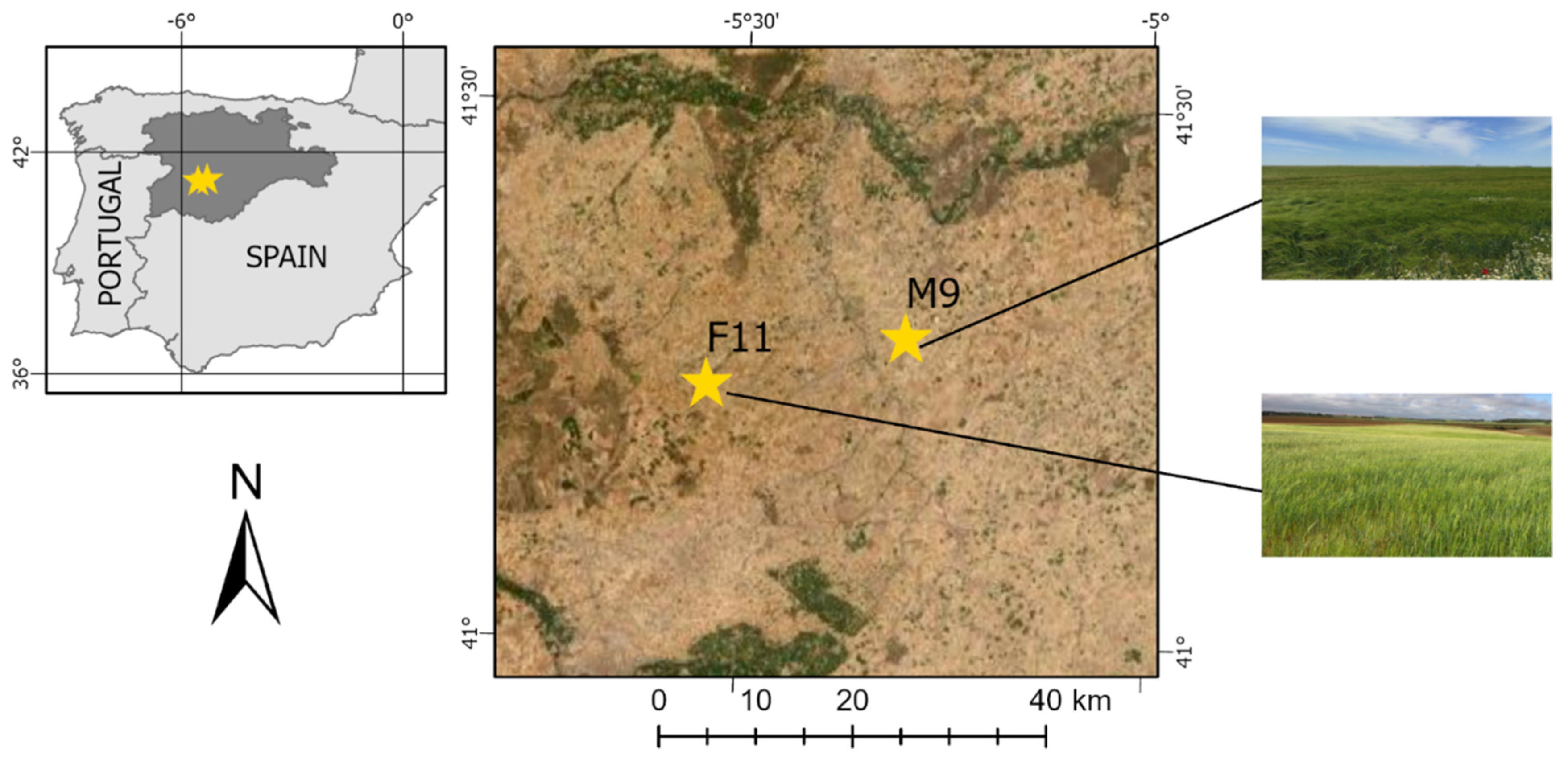
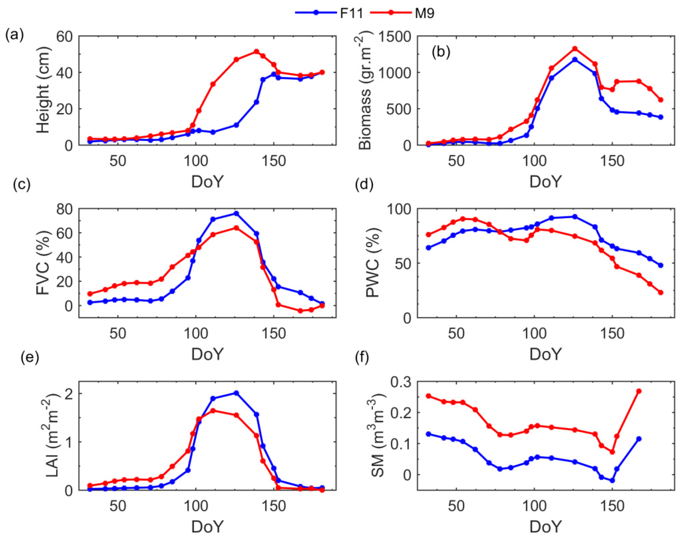
2.1. Study Area and Field Data

The Iberian Peninsula is extremely sensitive to future climate changes, especially the inner areas, where rainfed agriculture depends solely on rainfall. The study area (Figure 1) belongs to the central part of the Duero basin (41.1° to 41.5°N and 5.1° to 5.7°W), a fragile semi-arid area where a soil moisture station network (REMEDHUS) has been working since 1999, which is the property of the University of Salamanca in Spain. This network monitors the climatic and soil conditions of the area and provides ground data for agricultural and hydrological applications. A detailed description of the network, together with its agrometeorological equipment, is available in [44,45,46]. Two stations of REMEDHUS, namely F11 and M9 (Figure 1), were chosen in 2015 for a field campaign in their corresponding plots (both planted with barley) devoted to estimating field crop vegetation throughout their growing cycle. Soil moisture probes (Hydra Probes, Stevens Water Monitoring System, Inc.) provided a soil moisture dataset for each area, and the automatic weather stations of the network (Figure 1) supplied the meteorological data (precipitation, P, and evapotranspiration, ET0). The study spanned from February to June 2015, and the crops measurements were taken fortnightly (nine measurements in total). The objective of the campaign was to seek consistent relationships between ground measurements and remote-sensed SAR data acquired simultaneously by the RADARSAT-2 mission, as explained in the next section. Previous experiments successfully proved the relationships between both datasets using simple correlations [47].
The crop measurements (taken either in situ or in the laboratory) aimed to estimate the following parameters: height, FVC, LAI, fresh biomass, and percentage of water content (PWC). The FVC was estimated using supervised image classification of photographs taken zenithally over the canopy. For the LAI estimation, a binary-threshold segmentation was applied to the scanned leaf samples. Biomass and PWC were obtained by weighting the fresh/dry samples. Finally, the soil moisture (SM) records (in volumetric units) were retrieved from the REMEDHUS probes at the F11 and M9 stations daily. See [47,48] for a more detailed explanation of the measurements.
The field data were measured fortnightly over the study period (excepting the soil moisture, with daily records), producing a total of 9 observations. As the dates of the field observations and those of the satellite images did not coincide (because the satellite’s passage over the area is not known in advance), the image series was interpolated to fit in with the field observations, as explained in the next section.

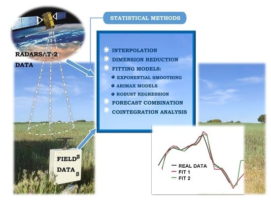
2.2. Satellite Data and Pre-Processing

RADARSAT-2 is a satellite launched by MacDonald, Dettwiler and Associates Ltd. (MDA) and the Canadian Space Agency (CSA) in December 2007. It has a C-band synthetic aperture radar (SAR) operating at 5.4 GHz, with multiple beam modes and an orbit repeat cycle of 24 days. For this study, a time series of 20 RADARSAT-2 images from February to July 2015 was acquired in Fine Quad-Pol Single Look Complex (SLC) from three different beam modes (FQ16W, FQ11W, and FQ6W) at different incidence angles (36°, 31°, and 25°) (Table 1).
As shown in Table 1, there is a mismatch between field measurements and RADARSAT-2 acquisition dates. This can be a source of uncertainty in the statistical analysis, especially when field measurements show trend changes or rapid changes; thus, a spline interpolation was applied to avoid this problem [47].
RADARSAT-2 data were processed using the Sentinel-1 Toolbox of the Sentinel Application Platform (SNAP, https://step.esa.int/main/toolboxes/snap/, accessed on 21 July 2020) provided by the European Space Agency (ESA) as follows: (1) radiometrically converting the images into backscattering coefficients using the look-up table from the images; (2) polarimetric coherency matrix generation [49]; (3) speckle filtering (9 × 9 boxcar); (4) terrain correction and geocoding using the Range Doppler orthorectification method and the digital elevation model from the Shuttle Radar Topographic Mission (SRTM); and (5) retrieving the polarimetric parameters using the PolSARpro software provided by the ESA (https://earth.esa.int/eogateway/tools/polsarpro, accessed on 21 July 2020). A detailed description of the procedure and parameters may be found in [47]. Table 2 summarizes both the polarimetric parameters and field observations, together with the weather records.

3. Methods

In order to adjust and predict the field measurements, different statistical techniques based on time series analysis were used, such as exponential smoothing on the in situ variables, ARIMAX, and regression by robust least squares. These methods were enriched with the contribution of potential meteorological explicative variables and linear combinations obtained from principal component analysis (PCA) of the satellite variables for each type of crop.
Once the adjustments and predictions of the aforementioned models were refined, the forecast combination methodology was used to obtain the final adjustment and prediction. Further, the cointegration method allows taking advantage of previous training to transfer the model to a new plot, provided the plot demonstrates a similar behaviour.

3.1. Interpolation

As previously mentioned, the dates of the field observations and satellite images do not coincide, so it seemed necessary to interpolate the data to compare the time series. Four data were taken per month starting in February 2015 and ending in June 2015. Since the meteorological records have a daily rate, weekly averages were also calculated to fit the temporal frequency of the other data. Twenty observations were used for the estimation models, and four were used for the prediction model.
Interpolation of missing data was carried out using cubic spline and least squares. Interpolation fits a cubic spline curve to the input values, which is a segmented function consisting of polynomial (cubic) functions joined so that the total curve and its first and second derivatives are continuous [50].

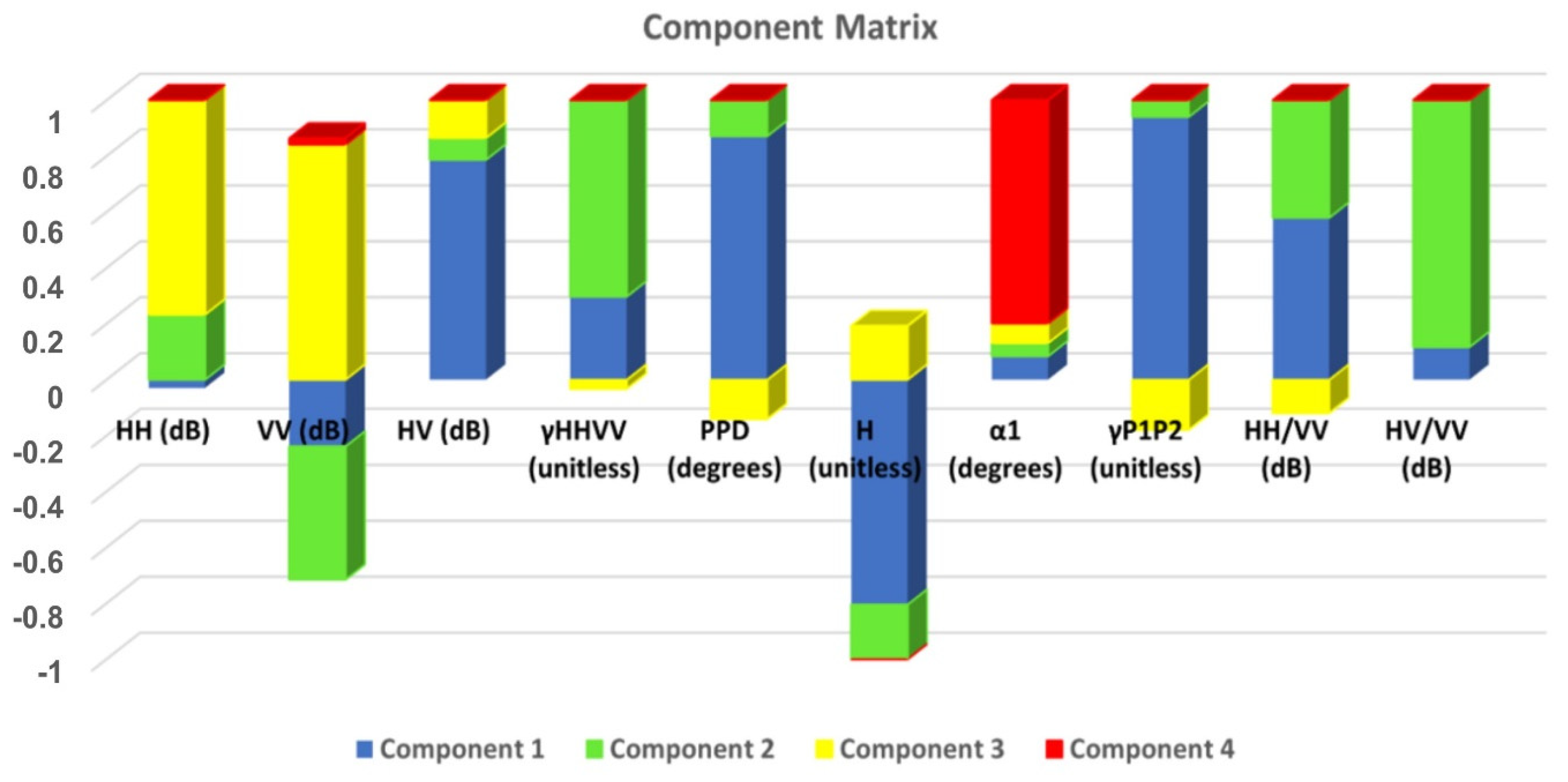
3.2. Dimension Reduction

Owing to the high number of parameters led by the images, the dimensionality of the information collected by these 10 satellite parameters was reduced by a principal component analysis. This methodology computes new variables as linear combinations of the original set, extracting the most relevant information in terms of variance. As a result, new variables (Factors) are calculated as linear combinations of the original variables. The first factor or principal component has the largest possible variance. The second component is calculated under the constraint of being orthogonal to the first component with the highest relevance, and so on. These components can be considered new axes representing the cloud of points that form the original variables. The projection of the points on the components serves to interpret the relationship between the different variables. If this interpretation is complex, the components (axes) can be rotated to redistribute the variance of the original variables in the factors to achieve a better interpretation of the results. For the rotation, the equamax rotation method is used, which minimizes the number of variables that contribute to a factor and the number of factors necessary to explain a variable [51,52,53].

3.3. Fitting Models

Several methodologies were used to adjust the time series of crop measurements, namely height, FVC, LAI, biomass, PWC, FVC, and SM. Exponential smoothing, which uses the information from the dynamics of the series, considers only the raw values of the field variables. The ARIMAX models also incorporate the information from the correlation of the white noise together with external variables such as the satellite variables (previously summarised in the factors obtained by the PCA) and meteorological variables. For field variables where the ARIMAX methodology did not provide a good fit, a robust regression was used to model them instead.

3.3.1. Exponential Smoothing

The simple exponential smoothing method is an evolution of the weighted moving average method. In this case, the average value of the time series is calculated using a self-correcting mechanism that aims to adjust the forecast in the opposite direction of the past deviation through the correction affected by the smoothing coefficient, α ∈ [0, 1]. This parameter controls the influence of the observations, i.e., large values indicate that the most recent past observations influence the forecasts the most, while smaller values mean that most of the historical data is considered when making a prediction. The single exponential smoothing method is appropriate for series that move randomly above and below a constant mean without trends or seasonal patterns [54]. A double smoothing adjustment was applied for each of the previously interpolated variables since they have a trend but no seasonality. This method repeats the single smoothing adjustment twice, appropriate for a series with a linear trend.
For a time series y t at instant t , we define:
S t = α y t + ( 1 α ) S t 1 D t = α S t + ( 1 α ) D t 1
where S t is the single smoothed series, D t is the double smoothed series, and α is the smoothing coefficient.
The forecast of a new observation at time t is computed as:
y T + k = ( 2 + α k 1 α ) S T ( 1 + α k 1 α ) D T = ( 2 S T D T + α 1 α ( S T D T ) k )

3.3.2. ARIMAX Models

ARIMAX models are ARIMA that incorporate exogenous variables into the adjustment. ARIMA are statistical models for time series that take into account the existing dependence between the data through its three components: autoregressive (AR), integrated (I), and moving averages (MA), which include cyclical or seasonal components and allow the description of the temporal variable as a linear function of previous data and errors due to randomness.
The general ARIMAX model is described by Equation (3):
( 1 B ) d y t = α + i = 1 p Φ i y t i + h = 1 q θ h ε t h + j = 1 r γ j X j + ε t
where B y t = y t 1 , d is the number of differences that must be applied to the series to make it stationary, α is the prerequisite for fitting an ARMA model using the Box Jenkins methodology, p is the number of autoregressive components in the equation and Φ i the associated parameter, X j is the model’s exogeneous variables and γ j the associated parameter, and ε t is the error at time t [55,56].
The Akaike information criterion (AIC) is used to determine which possible ARIMAX model is the best. This method serves to identify and select ARIMAX models as a measure of goodness-of-fit, which describes the relationship between the bias and variance in the model construction. It provides a means for comparison between models and a tool for model selection, with the best model being the one with the lowest AIC value [57].
The Ljung–Box test [58] was used to validate the assumptions of the model, i.e., that the residuals follow a time series where values in different time instants are not statistically correlated (white noise) and, therefore, have a constant power spectral density.

3.3.3. Robust Regression

The most used method to estimate the coefficients of linear regression is the least squares. This method, while optimal in the case of normally distributed errors, is very sensitive to the presence of outliers. To solve this problem, other, more robust estimation methods have been developed, which are less affected by the presence of atypical data, such as M-estimation [59], S-estimation [60], and MM-estimation [61], referred to hereafter as robust least squares methods.
To evaluate the accuracy of the forecasts from both the ARIMAX and robust regression models, measures of accuracy (mean absolute error (MAE) and Theil’s inequality coefficient (TIC)) were used. A Theil’s inequality coefficient of less than one confirms the model’s suitability for forecasting [62].

3.4. Forecast Combination Techniques

A combination of predictions made through different processes can improve the precision of a single prediction [63]: the more diverse the prediction model, the more accurate the prediction result. The combination of predictions aggregates the different forecasts obtained from each model into a single one as a weighted average of all the predictions by considering the information collected by each model individually, see [64,65,66].
Different prediction combination techniques were used [67]:
  • Weighted least squares (WLS) requires knowledge of the true values of the forecasted variable for some of the forecast period. It compares real values with predictions using the regression coefficients as weights. This method does not require that the underlying individual forecasts are unbiased, and the resulting average can lie outside the range of the underlying forecasts.
  • Weighted mean squared error (MSE) consists of making a weighted average giving greater weight to the predictions of the models with less mean squared error. Stock and Watson [68] propose MSE weighting, which compares individual forecasts with real values over a forecast period.
The mean squared error of each forecast is computed and used to form individual forecast weights:
w i = 1 M S E i k j = 1 N 1 M S E j k

3.5. Cointegration Analysis

Engle and Granger [69] developed the concept of cointegration, i.e., two series are said to be cointegrated if they move together over time, and the differences between them are stable. Hence, cointegration reflects the presence of a long-term equilibrium toward which the system converges over time. If more than two series are cointegrated, at least one must cause the other. The differences (or term error) in the cointegration equation are interpreted as the disequilibrium error for each particular point in time. Cointegration implies that there is a trend common to both series, so a properly weighted combination cancels this component. There is also a long-term equilibrium between both series, so deviations from equilibrium tend to disappear in relatively short terms.
A simple procedure to estimate the cointegration relationship consists of fitting a linear regression for the potentially cointegrated variables and then evaluating the stationarity of the residuals (constant mean and variance) that occurs in these data series. Different tests were used to analyze the feasibility of the cointegration:
  • The existence of cointegration between time series requires that each one is non-stationary, but the linear combination is stationary [70]. The augmented Dicky–Fuller test contrasts the null hypothesis for the existence of a unit root, equivalent to non-stationarity. To assess that both series are non-stationary, the augmented Dicky–Fuller test is used [56,71].
  • Granger’s causality test [72] checks whether the results of one variable serve to predict another variable analyzing the causal relationships between time series. Once this test is carried out, the cointegration equation is constructed, permitting one variable to be predicted using the results from another.
  • Johansen’s cointegration test [73,74] is another method to test the cointegration of several series. There are two types of Johansen tests, either with trace or with eigenvalue (maximum eigenvalue test). The inferences obtained with both alternatives may derive quite similar results; in this case, the results have been obtained with the trace.

4. Results

4.1. Dimension Reduction

After the series interpolation, PCA was performed to reduce the size of the satellite variables. The constructed factors are a linear combination of the original satellite variables: HH, HV, VV, HH/VV, HV/VV, γHHVV, PPD, H, α1, and γP1P2. An equamax rotation has been performed to improve the scoring of the satellite variables’ contributions for the factors. The results showed that the first four factors preserve 98% of the information in terms of cumulative variance, while the first two factors explain about 76% of the variability. Table 3 shows the coefficients of the linear combination of the satellite variable in each factor.
The constructed factors with the parameters associated with each variable according to the values are presented in Figure 2, indicating which variables have the greatest weight for each of the factors.
The incidence angle of the satellite observations was not used to subdivide the sample due to the scarcity of data. Of the 20 satellite data, 6 were observed with an angle of 25°, 7 with 31°, and 7 with 36°. However, the influence of the angle on the four new factors was analyzed employing an ANOVA test, using the angle as the factor. Table 4 shows the p-values of the tests for independence between the new variables and the angle and the associated Levene’s test for homogeneity of variances.
The results showed that the null hypothesis of homogeneity of variances was assumed in all cases (p-value > alpha = 0.05) for the Levene’s test, and there were no significant differences between Factors 1, 2, and 4 and the angle (p-value > alpha = 0.05) for the independence test, but significant differences were found for Factor 3.
Based on these results, of the four factors that explain 98% of the variability, the two that provide the greatest explanatory power while not being influenced by the angle (Factor 1 and Factor 2) were used as explanatory variables in the following adjustment models.

4.2. Analysis of Fitting Models over the Barley Crop on Field F11

In this section, the selected adjustment models described in Section 3 were evaluated to forecast the field variables (height, biomass, FVC, PWC, LAI, and SM) of the F11 crop field. When applied to the fittings, the meteorological variables (precipitation, evapotranspiration, and temperature) and the factors that summarize the satellite variables obtained from the principal component analysis were considered as explanatory variables. Once the adjustment models were obtained, the combination of predictions was carried out to obtain the final prediction.

4.2.1. Double Smoothing Adjustment

The double smoothing adjustment (Equation (1)) was performed for the field variables. Table 5 shows the fit coefficient (α), the residual sum of squares (RSS, which measures the amount of variance that is not explained by the model), and the mean squared difference between the estimated values and the true value: the mean squared error (MSE).
The α values near one highlighted the importance of the last measurements in the fitting model. This result agreed with the growing cycle behaviour of this crop, in which the last dates, corresponding to the fruit developing and ripening (around May), are vital for predicting the yield and final performance of the crop.

4.2.2. ARIMAX Adjustment and Robust Regression

The adjustment was carried out using ARIMAX models for the field variables. Table 6 presents the results of the models (parameters significant at 5%) with the lowest AIC, mean absolute error (MAE), MSE, and Theil’s inequality coefficient (TIC). The adequacy of the models for forecast purposes was confirmed by Theil’s inequality coefficient (<1), whereas the Ljung-Box assumed the hypothesis that the residuals are white noise at 5% and not autocorrelated. The results in Table 6 made clear that the influence of satellite variables (summarized in the constructed factors) was significant for all the considered measures to be estimated. Moreover, the adjustments are all dependent on the previous time instant, which is supported by the natural behaviour of barley plants, i.e., their state in a given moment is a consequence of the previous conditions.
As can be seen in Table 6, the dynamic structure of the time series for height was an ARIMAX (0,1,0) (Equation (5)). In this case, there was a positive impact of the two factors (F1t and F2t), dependence on the previous past observation (Ht−1), and a dynamic dependence with its lagged variable (εt). For the biomass variable, the fitting model was an ARIMAX (0,1,1) (Equation (6)), where there was a positive impact of the first factor and the ET0 variable, dependence on the previous instant (Bt−1), and a dynamic dependence of their errors. The ARIMAX highlighted the dependence of the biomass on the ET0. Equation (7) presents the estimation model for FVC, an ARIMAX (0,1,1), where there was a positive impact of F1 over FVC, dependence on the earlier time (FVCt−1), and a dynamic dependence of their errors. An ARIMAX (1,0,0) resulted for PWC (Equation (8)), where there was a positive impact of the first factor and temperature and a dynamic dependence on its own variable at the previous stage. Finally, the fit for LAI (Equation (9)) was an ARIMAX (0,1,1), and there was a positive impact of F1, dependence on the time instant past (LAIt−1), and a dynamic dependence on the errors.
In the case of the SM variable, the adjustment using ARIMAX models was not appropriate (TIC > 1 and adjustment coefficients not significant at 5%), so it was modelled using robust regression. The robust least squares estimation method allows better adjustments when there are outliers, as it is less sensitive to them. In this case, the S-estimation was used. After the estimation of this model for SM (Equation (10)), all resulting parameters were significant at the 0.05 level. A positive impact of F1 and the meteorological variables, ET0 and precipitation, took place for the SM. This is not surprising since the SM is the residual of the water inputs (rain) and outputs (ET0) of the soil–plant–atmosphere system [75]. The goodness-of-fit had an R-squared of 80%, the MAE was 0.02, the MSE was 0.83, and the TIC was 0.26.
SMt = 0.16 + 0.02 F1t + 0.03 ET0t + 0.96 Pt + εt

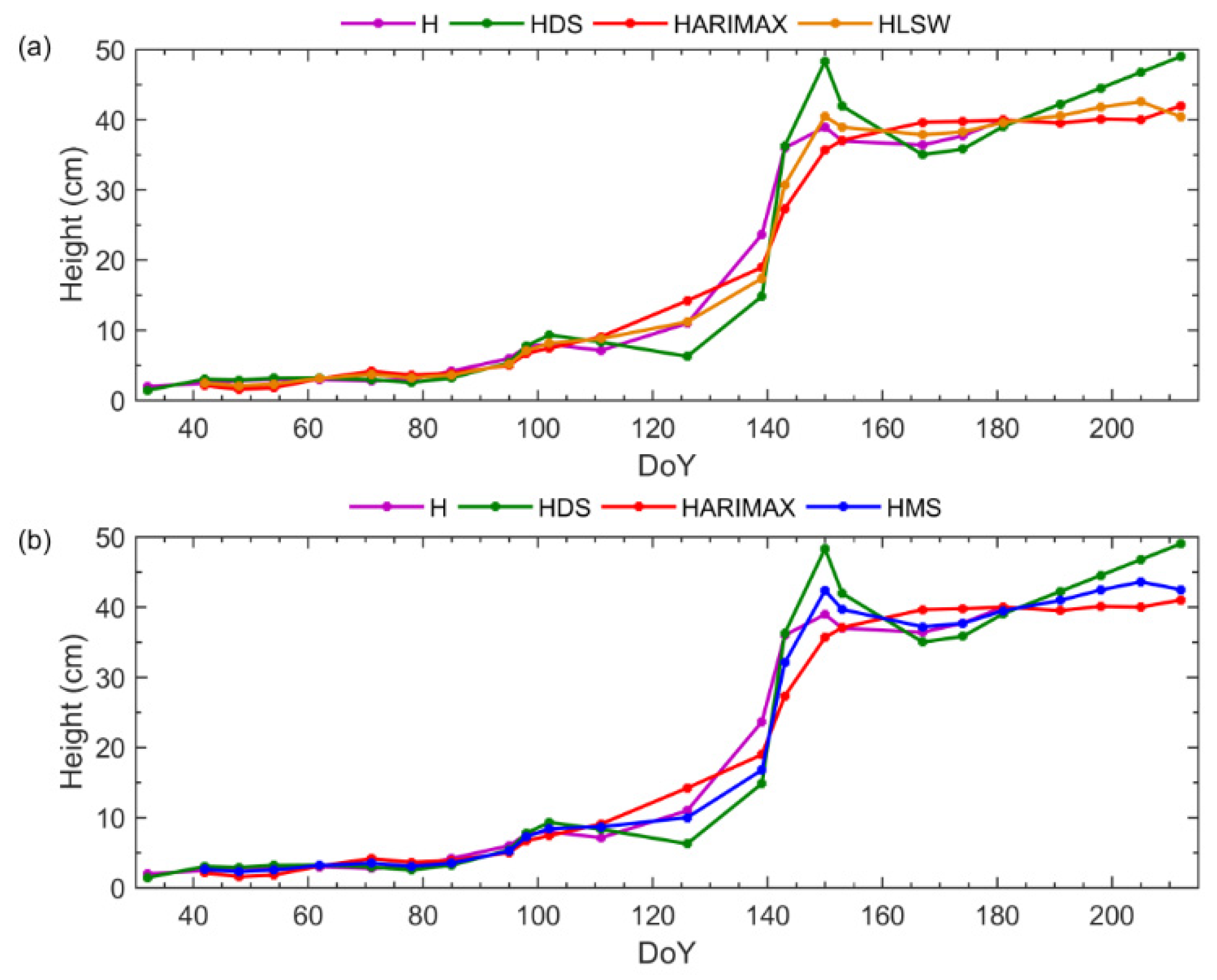
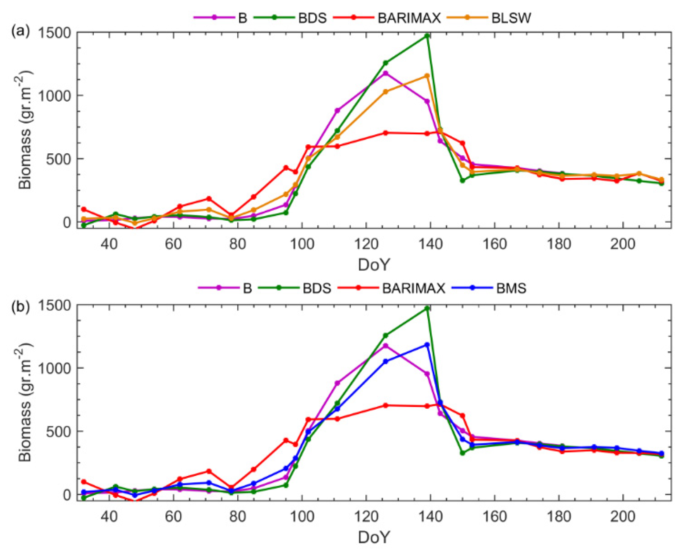
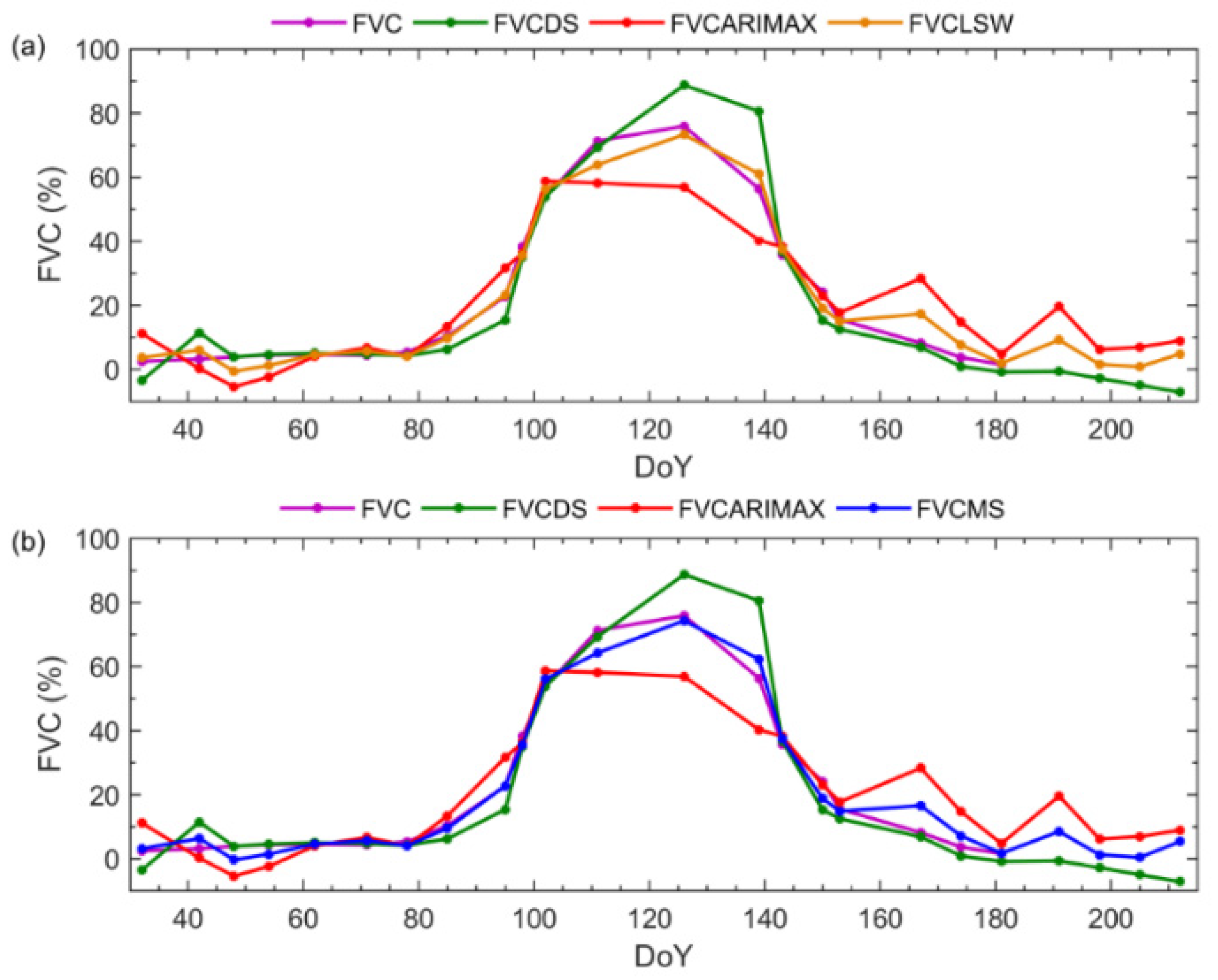
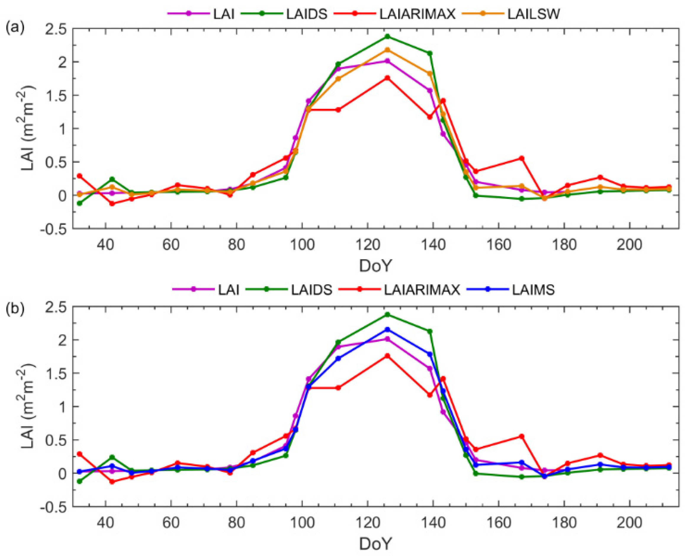
4.2.3. Combination of Forecasts

In the previous subsections, two models have been obtained for the adjustment and prediction of the field variables, double smoothing, and ARIMAX/robust regression. Thus, two different predictions for each field variable were available. To obtain the final prediction, a combination of the two predictions was made using the weighted least squares (LSW) and mean squared (MS) methods. Table 7 shows the mean squared error (MSE) of both methods for each field variable. As demonstrated, these results have a lower MSE than that obtained for the predictions of the individual models, double smoothing, and ARIMAX/robust regression (Table 6). The LSW is the method with the lowest MSE.
Figure 3, Figure 4, Figure 5, Figure 6, Figure 7 and Figure 8 show the results of the model adjustments. The results obtained show the goodness-of-fit and its feasibility to predict.

4.3. Prediction of Biophysical Variables of Barley on M9

Since the time evolution of barley in plots F11 and M9 is similar for all field variables (Figure 9), a cointegration may be expected. Thus, the results obtained for F11 may be used to adjust and predict those of plot M9.
To ensure that cointegration is possible, the three tests described in Section 3.5 were applied to both series. The results of the augmented Dicky–Fuller test showed that all the series were non-stationary. In all cases, the null hypothesis of non-stationarity at 5% was accepted, and the p-values were height (0.99), biomass (0.39), FVC (0.18), PWC (0.95), LAI (0.16), and SM (0.16). Granger’s causality test found a bidirectional relationship between the same measures of the two fields at a significance level of 5%. Granger’s causality test assumes the null hypothesis that the second series does not cause the first series with a certain time lag. Thus, if p-values below the significance level are obtained (p-value < alpha = 0.05), the hypothesis can be rejected, concluding that causality exists: height (p-value = 0.014), biomass (p-value = 0.04), FVC (p-value = 0.005), PWC (p-value = 0.003), LAI (p-value = 0.01), and SM (p-value = 0.02). Finally, the Johansen cointegration test reflects at 5% the existence of cointegration relationships between the two fields. The Johansen cointegration test shows that the null hypothesis of cointegration between the series is assumed in all cases (p-value > alpha = 0.05): height (p-value = 0.20), biomass (p-value = 0.09), FVC (p-value = 0.10), PWC (p-value = 0.30), LAI (p-value = 0.36), and SM (p-value = 0.22).
Therefore, it seemed unnecessary to repeat the adjustments in plot M9 for each field variable since the predictions of the modelling of plot F11 would be used to predict plot M9 with the cointegration equation. Table 8 shows the fit of the field measurements of the two plots by the cointegration equations, indicating a stable linear relationship. Furthermore, the residuals of the regression were stationary, which indicated the fit robustness. Figure 10 shows the results of the biophysical variables of M9 adjusted by cointegration through the data of the F11 plot.

5. Discussion

To develop efficient adjustment and prediction models for the biophysical variables of crops, it is necessary to have a good dataset, including meteorological data, to fulfil the remote sensing series and the in situ measurements. Prior to analyzing the datasets, an interpolation had to be carried out to be able to compare the data series over time. The satellite data provide many variables, so they are clustered using PCA to obtain factors that explain a high percentage of the variability of these variables. These factors were used as exogenous variables in the adjustment and the rest of the meteorological variables. The weather data was shown to be especially helpful in the case of the soil moisture adjustment, although this variable is one of the most typically retrieved from radar data [76]. Moreover, ARIMAX highlighted the dependence of both the biomass on the ET0, as it is recognized and applied in many crop models [77,78], and the temperature as an indicator of the water status of plants and soils jointly with the FVC [79,80,81].
To choose the most appropriate method for modelling and predicting each of the field variables (heigh, biomass, FVC, PWC, LAI, and SM), comparing different statistical methodologies is necessary to finally choose the two models with the best results for each field variable (double smoothing and ARIMAX/robust regression). Once the adjustment and forecast was performed with the chosen models, the accuracy was improved using the combined predictions. In this study, different methodologies were tested and compared to obtain the best fit for LSW. To date, this method has been scarcely applied to SAR data. Statistical methods have usually been applied for crop classification [82] or to characterize polarimetric parameters [83,84]; however, statistical modelling is rare. Not surprisingly, Yuzugullu et al. [85] stated that “most of the current statistical methods are not capable of explaining the growth cycle of rice crops in different areas while avoiding high training costs”. We tried to show effective statistical modelling with limited field data and without training to fit the growing cycle of several parameters of barley.
The statistical analysis carried out for one of the barley plots can be extrapolated to the other. Considering the specific characteristics derived from the same crop, the analysis of the cointegration existing between the data series of both plots (F11 and M9) allows adjusting the field variables of one through the adjustments made in the other.
The results obtained show the suitable adjustments made with the different statistical methods used, despite having a small sample of field data and many satellite variables. Therefore, the use of satellite images makes it possible to adjust the field variables, avoiding costly in situ measurements. For this reason, the field measurements are usually scarce in comparison with SAR observations and, therefore, limit other fitting methods such as simple regression, as done in Maity et al. [86] (three measurements over cotton), Lim et al. [87] (six measurements over rice) and our previous application with the same dataset [47].
In comparison with the results of the reviewed literature where statistical time series methodologies are used, the novelty of this paper is that these were performed with data obtained from remotely sensed observations, together with field data and meteorological variables. In addition, the best fitting models are combined, and, using cointegration techniques, the results are extrapolated to other fields.
As ideas for further research, different machine learning methodologies could be used if a large amount of satellite data is available and to compare fields with different crop types.

6. Conclusions

This research showed a statistical procedure for modelling and predicting crop biophysical variables with time series of SAR images. Although the method is well-known in the statistical community, it was never applied to temporal series retrieved from remote sensing observations. The strategy is specifically convenient when the temporal series of field data, usually accompanying the image series, are short or scarce, a situation rather frequent owing to the difficulty of gathering field observations.
The real dimensionality of image variable parameters was reduced by the PCA analysis, obtaining four factors that could explain 98% of the variability of the satellite variables, among which only the first two factors were relevant in the model.
The field data were modelled and adjusted by several statistical procedures (double smoothing, ARIMAX, and robust regression), generating two models with their corresponding coefficients, influence variables, and predictions for each field variable (height, biomass, FVC, PWC, LAI, and SM). The model equations showed a positive contribution of the meteorological variables, in particular, ET0 and precipitation for SM, ET0 for the biomass, and temperature for PWC. Further, the modelled series noted the importance of the crop status from one measurement to the next, highlighting the strong temporal component in crop development. The contributions found in the modelling reflect the dependence between the crop parameters and the effect of time, mirroring the real behaviour of this crop. The combination of the predictions obtained for the field variables by the two models improves the accuracy of the predictions. To make the combination of predictions, the weighted least squares (LSW) and the mean squared (MS) methods were tested and compared, concluding that the LSW provides a better fit.
Cointegration is an interesting tool to avoid replicating the model for different crops. In this case, the M9 field variables were fitted with the data from field F11, both producing barley.
The methodology employed is very popular with economic data, where different model adjustments are made to subsequently combine them to obtain the best possible fit. Moreover, cointegration between time series is commonly performed in econometrics. In this case, despite the small sample of filed data, the procedures have provided good results.
Alternative methods of statistical fitting applied between fields and remote sensing images pave the way to use the imagery as a subrogate of the crop behaviour, avoiding time-consuming field measurements.

Author Contributions

All authors contributed significantly to this manuscript. Conceptualization, A.E.S., M.T.S.-M. and C.S.d.B.; methodology, A.E.S.; validation, N.S. and R.V.-D.; formal analysis, A.E.S., M.T.S.-M. and C.S.d.B.; investigation, A.E.S., M.T.S.-M. and C.S.d.B.; resources, N.S.; data curation, A.E.S., M.T.S.-M., R.V.-D. and C.S.d.B.; writing—original draft preparation, A.E.S.; writing—review and editing, all. All authors have read and agreed to the published version of the manuscript.

Funding

This study was supported by the Spanish Ministry of Science and Innovation (projects ESP2017-89463-C3-3-R, PID2019-108311GB-I00/AEI/10.13039/501100011033, and PID2020-114623RB-C33), the Castilla y León Government (projects SA112P20, SA105P20, and CLU-2018-04)and the European Regional Development Fund (ERDF).

Conflicts of Interest

The authors declare no conflict of interest.

References

  1. Yu, R.; Evans, A.J.; Malleson, N. Quantifying grazing patterns using a new growth function based on MODIS Leaf Area Index. Remote Sens. Environ. 2018, 209, 181–194. [Google Scholar] [CrossRef] [Green Version]
  2. Champagne, C.; White, J.; Berg, A.; Belair, S.; Carrera, M. Impact of soil moisture data characteristics on the sensitivity to crop yields under drought and excess moisture conditions. Remote Sens. 2019, 11, 372. [Google Scholar] [CrossRef] [Green Version]
  3. Habyarimana, E.; Piccard, I.; Catellani, M.; De Franceschi, P.; Dall’Agata, M. Towards predictive modeling of sorghum biomass yields using fraction of absorbed photosynthetically active radiation derived from sentinel-2 satellite imagery and supervised machine learning techniques. Agronomy 2019, 9, 203. [Google Scholar] [CrossRef] [Green Version]
  4. White, J.; Berg, A.A.; Champagne, C.; Zhang, Y.; Chipanshi, A.; Daneshfar, B. Improving crop yield forecasts with satellite-based soil moisture estimates: An example for township level canola yield forecasts over the Canadian Prairies. Int. J. Appl. Earth Obs. Geoinf. 2020, 89, 102092. [Google Scholar] [CrossRef]
  5. Brocca, L.; Ciabatta, L.; Massari, C.; Camici, S.; Tarpanelli, A. Soil moisture for hydrological applications: Open questions and new opportunities. Water 2017, 9, 140. [Google Scholar] [CrossRef]
  6. Martínez-Fernández, J.; González-Zamora, A.; Sánchez, N.; Gumuzzio, A.; Herrero-Jiménez, C.M. Satellite soil moisture for agricultural drought monitoring: Assessment of the SMOS derived Soil Water Deficit Index. Remote Sens. Environ. 2016, 177, 277–286. [Google Scholar] [CrossRef]
  7. Martínez-Fernández, J.; Sánchez, N.; González-Zamora, Á. Agricultural drought monitoring using satellite soil moisture and other remote sensing data over the Iberian Peninsula. In Remote Sensing of Hydrometeorological Hazards; Petropoulos, G.P., Islam, T., Eds.; CRC Press, Taylor & Francis Group: Boca Raton, FL, USA, 2017; p. 549. ISBN 9781498777599. [Google Scholar]
  8. Sánchez, N.; González-Zamora, Á.; Martínez-Fernández, J.; Piles, M.; Pablos, M. Integrated remote sensing approach to global agricultural drought monitoring. Agric. For. Meteorol. 2018, 259, 141–153. [Google Scholar] [CrossRef]
  9. Sánchez, N.; González-Zamora, Á.; Piles, M.; Martínez-Fernández, J. A new Soil Moisture Agricultural Drought Index (SMADI) integrating MODIS and SMOS products: A case of study over the Iberian Peninsula. Remote Sens. 2016, 8, 287. [Google Scholar] [CrossRef] [Green Version]
  10. Mousivand, A.; Menenti, M.; Gorte, B.; Verhoef, W. Multi-temporal, multi-sensor retrieval of terrestrial vegetation properties from spectral-directional radiometric data. Remote Sens. Environ. 2015, 158, 311–330. [Google Scholar] [CrossRef]
  11. Campos-Taberner, M.; Moreno-Martínez, Á.; García-Haro, F.J.; Camps-Valls, G.; Robinson, N.P.; Kattge, J.; Running, S.W. Global estimation of biophysical variables from Google Earth Engine platform. Remote Sens. 2018, 10, 1167. [Google Scholar] [CrossRef] [Green Version]
  12. Djamai, N.; Fernandes, R.; Weiss, M.; McNairn, H.; Goïta, K. Validation of the Sentinel Simplified Level 2 Product Prototype Processor (SL2P) for mapping cropland biophysical variables using Sentinel-2/MSI and Landsat-8/OLI data. Remote Sens. Environ. 2019, 225, 416–430. [Google Scholar] [CrossRef]
  13. Upreti, D.; Huang, W.; Kong, W.; Pascucci, S.; Pignatti, S.; Zhou, X.; Ye, H.; Casa, R. A comparison of hybrid machine learning algorithms for the retrieval of wheat biophysical variables from Sentinel-2. Remote Sens. 2019, 11, 481. [Google Scholar] [CrossRef] [Green Version]
  14. Xie, Q.; Dash, J.; Huete, A.; Jiang, A.; Yin, G.; Ding, Y.; Peng, D.; Hall, C.C.; Brown, L.; Shi, Y.; et al. Retrieval of crop biophysical parameters from Sentinel-2 remote sensing imagery. Int. J. Appl. Earth Obs. Geoinf. 2019, 80, 187–195. [Google Scholar] [CrossRef]
  15. Ulaby, F.T. Radar response to vegetation. IEEE Trans. Antennas Propag. 1975, 23, 36–45. [Google Scholar] [CrossRef]
  16. Ulaby, F.T.; Bush, T.F.; Batlivala, P.P. Radar response to vegetation II: 8–18 GHz band. IEEE Trans. Antennas Propag. 1975, 23, 608–618. [Google Scholar] [CrossRef]
  17. Liu, C.A.; Chen, Z.X.; Shao, Y.; Chen, J.S.; Hasi, T.; Pan, H. Research advances of SAR remote sensing for agriculture applications: A review. J. Integr. Agric. 2019, 18, 506–525. [Google Scholar] [CrossRef] [Green Version]
  18. Moran, M.S.; Alonso, L.; Moreno, J.F.; Cendrero Mateo, M.P.; de la Cruz, D.F.; Montoro, A. A RADARSAT-2 quad-polarized time series for monitoring crop and soil conditions in Barrax, Spain. IEEE Trans. Geosci. Remote Sens. 2012, 50, 1057–1070. [Google Scholar] [CrossRef]
  19. Vreugdenhil, M.; Wagner, W.; Bauer-Marschallinger, B.; Pfeil, I.; Teubner, I.; Rüdiger, C.; Strauss, P. Sensitivity of Sentinel-1 backscatter to vegetation dynamics: An Austrian case study. Remote Sens. 2018, 10, 1396. [Google Scholar] [CrossRef] [Green Version]
  20. Attema, E.P.W.; Ulaby, F.T. Vegetation modeled as a water cloud. Radio Sci. 1978, 13, 357–364. [Google Scholar] [CrossRef]
  21. Hosseini, M.; McNairn, H. Using multi-polarization C- and L-band synthetic aperture radar to estimate biomass and soil moisture of wheat fields. Int. J. Appl. Earth Obs. Geoinf. 2017, 58, 50–64. [Google Scholar] [CrossRef]
  22. Ulaby, F.T.; Batlivala, P.P.; Dobson, M.C. Microwave backscatter dependence on surface roughness, soil moisture, and soil texture: Part I–bare soil. IEEE Trans. Geosci. Electron. 1978, 16, 286–295. [Google Scholar] [CrossRef]
  23. Guo, X.; Li, K.; Shao, Y.; Wang, Z.; Li, H.; Yang, Z.; Liu, L.; Wang, S. Inversion of rice biophysical parameters using simulated compact polarimetric sar c-band data. Sensors 2018, 18, 2271. [Google Scholar] [CrossRef] [Green Version]
  24. Mandal, D.; Kumar, V.; Lopez-Sanchez, J.M.; Bhattacharya, A.; McNairn, H.; Rao, Y.S. Crop biophysical parameter retrieval from Sentinel-1 SAR data with a multi-target inversion of Water Cloud Model. Int. J. Remote Sens. 2020, 41, 5503–5524. [Google Scholar] [CrossRef]
  25. Chen, K.S.; Yen, S.K.; Huang, W.P. A simple model for retrieving bare soil moisture from radar-scattering coefficients. Remote Sens. Environ. 1995, 54, 121–126. [Google Scholar] [CrossRef]
  26. Shi, J.; Wang, J.; Hsu, A.Y.; O’Neill, P.E.; Engman, E.T. Estimation of bare surface soil moisture and surface roughness parameter using L-band SAR image data. IEEE Trans. Geosci. Remote Sens. 1997, 35, 1254–1266. [Google Scholar] [CrossRef]
  27. Oh, Y.; Sarabandi, K.; Ulaby, F.T. Semi-empirical model of the ensemble-averaged differential Mueller matrix for microwave backscattering from bare soil surfaces. IEEE Trans. Geosci. Remote Sens. 2002, 40, 1348–1355. [Google Scholar] [CrossRef] [Green Version]
  28. Oh, Y. Quantitative retrieval of soil moisture content and surface roughness from multipolarized radar observations of bare soil surfaces. IEEE Trans. Geosci. Remote Sens. 2004, 42, 596–601. [Google Scholar] [CrossRef]
  29. Álvarez-Mozos, J.; González-Audícana, M.; Casalí, J. Evaluation of empirical and semi-empirical backscattering models for surface soil moisture estimation. Can. J. Remote Sens. 2007, 33, 176–188. [Google Scholar] [CrossRef]
  30. Wang, H.; Méric, S.; Allain, S.; Pottier, E. Adaptation of Oh Model for soil parameters retrieval using multi-angular RADARSAT-2 datasets. J. Surv. Mapp. Eng. 2014, 2, 65–74. [Google Scholar]
  31. Fung, A.K.; Chen, K.S. Dependence of the surface backscattering coefficients on roughness, frequency and polarization states. Int. J. Remote Sens. 1992, 13, 1663–1680. [Google Scholar] [CrossRef]
  32. Ulaby, F.T.; Moore, R.K.; Fung, A.K. Microwave Remote Sensing: Active and Passive/Volume II, Radar Remote Sensing and Surface Scattering and Emission Theory; Addison-Wesley: Reading, MA, USA, 1982. [Google Scholar]
  33. Fung, A.K.; Chen, K.S. An update on the IEM surface backscattering model. IEEE Geosci. Remote Sens. Lett. 2004, 1, 75–77. [Google Scholar] [CrossRef]
  34. Der Wu, T.; Chen, K.S.; Shi, J.; Fung, A.K. A transition model for the reflection coefficient in surface scattering. IEEE Trans. Geosci. Remote Sens. 2001, 39, 2040–2050. [Google Scholar] [CrossRef]
  35. Lievens, H.; Verhoest, N.E.C. On the retrieval of soil moisture in wheat fields from L-band SAR based on water cloud modeling, the IEM, and effective roughness parameters. IEEE Geosci. Remote Sens. Lett. 2011, 8, 740–744. [Google Scholar] [CrossRef]
  36. Bai, X.; He, B.; Xing, M.; Li, X. Method for soil moisture retrieval in arid prairie using TerraSAR-X data. J. Appl. Remote Sens. 2015, 9, 096062. [Google Scholar] [CrossRef]
  37. Bai, X.; He, B.; Li, X.; Zeng, J.; Wang, X.; Wang, Z.; Zeng, Y.; Su, Z. First assessment of Sentinel-1A data for surface soil moisture estimations using a coupled water cloud model and advanced integral equation model over the Tibetan Plateau. Remote Sens. 2017, 9, 714. [Google Scholar] [CrossRef] [Green Version]
  38. Mestre-Quereda, A.; Lopez-Sanchez, J.M.; Vicente-Guijalba, F.; Jacob, A.W.; Engdahl, M.E. Time Series of Sentinel-1 Interferometric Coherence and Backscatter for Crop-Type Mapping. IEEE J. Sel. Top. Appl. Earth Obs. Remote Sens. 2020, 13, 4070–4084. [Google Scholar] [CrossRef]
  39. Nasirzadehdizaji, R.; Cakir, Z.; Balik Sanli, F.; Abdikan, S.; Pepe, A.; Calò, F. Sentinel-1 interferometric coherence and backscattering analysis for crop monitoring. Comput. Electron. Agric. 2021, 185, 106118. [Google Scholar] [CrossRef]
  40. Shang, J.; Liu, J.; Poncos, V.; Geng, X.; Qian, B.; Chen, Q.; Dong, T.; Macdonald, D.; Martin, T.; Kovacs, J.; et al. Detection of crop seeding and harvest through analysis of time-series Sentinel-1 interferometric SAR data. Remote Sens. 2020, 12, 1551. [Google Scholar] [CrossRef]
  41. Jiang, B.; Liang, S.; Wang, J.; Xiao, Z. Modeling MODIS LAI time series using three statistical methods. Remote Sens. Environ. 2010, 114, 1432–1444. [Google Scholar] [CrossRef]
  42. Han, P.; Wang, P.X.; Zhang, S.Y.; Zhu, D.H. Drought forecasting based on the remote sensing data using ARIMA models. Math. Comput. Model. 2010, 51, 1398–1403. [Google Scholar] [CrossRef]
  43. Fernández-Manso, A.; Quintano, C.; Fernández-Manso, O. Forecast of NDVI in coniferous areas using temporal ARIMA analysis and climatic data at a regional scale. Int. J. Remote Sens. 2011, 32, 1595–1617. [Google Scholar] [CrossRef]
  44. González-Zamora, A.; Sánchez, N.; Martínez-Fernández, J. Validation of Aquarius soil moisture products over the Northwest of Spain: A comparison with SMOS. IEEE J. Sel. Top. Appl. Earth Obs. Remote Sens. 2016, 9, 2763–2769. [Google Scholar] [CrossRef]
  45. Martínez-Fernández, J.; González-Zamora, A.; Almendra-Martín, L. Soil moisture memory and soil properties: An analysis with the stored precipitation fraction. J. Hydrol. 2021, 593, 125622. [Google Scholar] [CrossRef]
  46. Sánchez, N.; Martínez-Fernández, J.; Scaini, A.; Pérez-Gutiérrez, C. Validation of the SMOS L2 Soil Moisture Data in the REMEDHUS Network (Spain). IEEE Trans. Geosci. Remote Sens. 2012, 50, 1602–1611. [Google Scholar] [CrossRef]
  47. Valcarce-Diñeiro, R.; Lopez-Sanchez, J.M.; Sánchez, N.; Arias-Pérez, B.; Martínez-Fernández, J. Influence of incidence angle in the correlation of C-band polarimetric parameters with biophysical variables of rain-fed crops. Can. J. Remote Sens. 2018, 44, 643–659. [Google Scholar] [CrossRef]
  48. Sánchez, N.; Martínez-Fernández, J.; González-Piqueras, J.; González-Dugo, M.P.; Baroncini-Turrichia, G.; Torres, E.; Calera, A.; Pérez-Gutiérrez, C. Water balance at plot scale for soil moisture estimation using vegetation parameters. Agric. For. Meteorol. 2012, 166–167, 1–9. [Google Scholar] [CrossRef]
  49. Cloude, S.R.; Pottier, E. A review of target decomposition theorems in radar polarimetry. IEEE Trans. Geosci. Remote Sens. 1996, 34, 498–518. [Google Scholar] [CrossRef]
  50. Quintero Salazar, E.; Urueña, W.; Gallego Becerra, H. Interfaz gráfica para la interpolación de datos a través de Splines Cúbicos. Sci. Tech. 2010, 1, 195–200. [Google Scholar] [CrossRef]
  51. Hotelling, H. Analysis of a complex of statistical variables into principal components. J. Educ. Psychol. 1933, 24, 417–441. [Google Scholar] [CrossRef]
  52. Jackson, J.E. A User’s Guide to Principal Components; John Wiley & Sons, Inc.: New York, NY, USA, 1991. [Google Scholar]
  53. Jolliffe, I. Principal Component Analysis, 2nd ed.; Springer: New York, NY, USA, 2002; ISBN 978-0-387-95442-4. [Google Scholar]
  54. Gardner, E.S. Exponential smoothing: The state of the art. J. Forecast. 1985, 4, 1–28. [Google Scholar] [CrossRef]
  55. Box, G.E.P.; Jenkins, G.M. Time Series Analysis: Forecasting and Control; Holden-Day: San Francisco, CA, USA, 1970; ISBN 0816210942. [Google Scholar]
  56. Hamilton, J.D. Time Series Analysis; Princeton University Press: Princeton, NJ, USA, 1994; ISBN 0691042896. [Google Scholar]
  57. Brockwell, P.J.; Davis, R.A. Time Series: Theory and Methods, 2nd ed.; Springer: New York, NY, USA, 1991; ISBN 978-0-387-97429-3. [Google Scholar]
  58. Ljung, G.M.; Box, G.E.P. On a measure of lack of fit in time series models. Biometrika 1978, 65, 297–303. [Google Scholar] [CrossRef]
  59. Huber, P.J. Robust regression: Asymptotics, conjectures and Monte Carlo. Ann. Stat. 1973, 1, 799–821. [Google Scholar] [CrossRef]
  60. Rousseeuw, P.; Yohai, V. Robust regression by means of S-estimators. In Robust and Nonlinear Time Series Analysis; Springer: New York, NY, USA, 1984; pp. 256–272. [Google Scholar]
  61. Yohai, V.J. High breakdown-point and high efficiency robust estimates for regression. Ann. Stat. 1987, 15, 642–656. [Google Scholar] [CrossRef]
  62. Fair, R.C. Evaluating the predictive accuracy of models. In Handbook of Econometrics; Griliches, Z., Intriligator, M.D., Eds.; Elsevier: Amsterdam, The Netherlands, 1986; pp. 1979–1995. [Google Scholar]
  63. Bates, J.; Granger, C.W. The combination of forecasts. Oper. Res. Q. 1969, 20, 451–468. [Google Scholar] [CrossRef]
  64. Clemen, R.T. Combining forecasts: A review and annotated bibliography. Int. J. Forecast. 1989, 5, 559–583. [Google Scholar] [CrossRef]
  65. Makridakis, S.; Hibon, M. The M3-competition: Results, conclusions and implications. Int. J. Forecast. 2000, 16, 451–476. [Google Scholar] [CrossRef]
  66. Timmermann, A. Forecast combinations. In Handbook of Economic Forecasting; Granger, C.W.J., Elliot, G., Timmermann, A., Eds.; Elsevier: Amsterdam, The Netherlands, 2006; pp. 135–196. [Google Scholar]
  67. Granger, C.W.J.; Elliot, G.; Timmermann, A. Handbook of Economic Forecasting; Elsevier: Amsterdam, The Netherlands, 2006. [Google Scholar]
  68. Stock, J.H.; Watson, M.W. Vector autoregressions. J. Econ. Perspect. 2001, 15, 101–105. [Google Scholar] [CrossRef] [Green Version]
  69. Engle, R.F.; Granger, C.W.J. Co-integration and error correction: Representation, estimation, and testing. Econometrica 1987, 55, 251–276. [Google Scholar] [CrossRef]
  70. Perman, R. Cointegration: An Introduction to the literature. J. Econ. Stud. 1991, 18. [Google Scholar] [CrossRef]
  71. Dickey, D.A.; Fuller, W.A. Distribution of the estimators for autoregressive time series with a unit root. J. Am. Stat. Assoc. 1979, 74, 427–431. [Google Scholar] [CrossRef]
  72. Granger, C.W.J. Investigating causal relations by econometric models and cross-spectral methods. Econometrica 1969, 37, 424–438. [Google Scholar] [CrossRef]
  73. Johansen, S. Estimation and hypothesis testing of cointegration vectors in gaussian vector autoregressive models. Econometrica 1991, 59, 1551–1580. [Google Scholar] [CrossRef]
  74. Johansen, S. Likelihood-Based Inference in Cointegrated Vector Autoregressive Models; Oxford University Press: Oxford, UK, 1995; ISBN 9780198774501. [Google Scholar]
  75. Allen, R.G.; Pereira, L.S.; Raes, D.; Smith, M. Crop Evapotranspiration—Guidelines for Computing Crop Water Requirements—FAO Irrigation and Drainage Paper 56; FAO: Rome, Italy, 1998.
  76. Khabbazan, S.; Vermunt, P.; Steele-Dunne, S.; Arntz, L.R.; Marinetti, C.; van der Valk, D.; Iannini, L.; Molijn, R.; Westerdijk, K.; van der Sande, C. Crop monitoring using Sentinel-1 data: A case study from The Netherlands. Remote Sens. 2019, 11, 1887. [Google Scholar] [CrossRef] [Green Version]
  77. Raes, D.; Steduto, P.; Hsiao, T.C.; Fereres, E. Aquacrop-The FAO crop model to simulate yield response to water: II. main algorithms and software description. Agron. J. 2009, 101, 438–447. [Google Scholar] [CrossRef] [Green Version]
  78. Bauböck, R. Simulating the yields of bioenergy and food crops with the crop modeling software BioSTAR: The carbon-based growth engine and the BioSTAR ET0 method. Environ. Sci. Eur. 2014, 26, 26. [Google Scholar] [CrossRef] [Green Version]
  79. Carlson, T.N.; Gillies, R.R.; Perry, E.M. A method to make use of thermal infrared temperature and NDVI measurements to infer surface soil water content and fractional vegetation cover. Remote Sens. Rev. 1994, 9, 161–173. [Google Scholar] [CrossRef]
  80. Moran, M.S.; Maas, S.J.; Vanderbilt, V.C.; Barnes, E.M.; Miller, S.N.; Clarke, T.R. Application of image based remote sensing to irrigated agriculture. In Remote Sensing for Natural Resources Management and Environmental Monitoring: Manual of Remote Sensing; Ustin, S.L., Ed.; John Wiley & Sons, Inc.: London, UK, 2004; pp. 617–676. [Google Scholar]
  81. Sandholt, I.; Rasmussen, K.; Andersen, J. A simple interpretation of the surface temperature/vegetation index space for assessment of surface moisture status. Remote Sens. Environ. 2002, 79, 213–224. [Google Scholar] [CrossRef]
  82. Soares, J.V.; Rennó, C.D.; Formaggio, A.R.; Yanasse, C.D.C.F.; Frery, A.C. An investigation of the selection of texture features for crop discrimination using SAR imagery. Remote Sens. Environ. 1997, 59, 234–247. [Google Scholar] [CrossRef]
  83. Erten, E.; Rossi, C.; Yüzügüllü, O. Polarization Impact in TanDEM-X Data over Vertical-Oriented Vegetation: The Paddy-Rice Case Study. IEEE Geosci. Remote Sens. Lett. 2015, 12, 1501–1505. [Google Scholar] [CrossRef] [Green Version]
  84. Inoue, Y.; Kurosu, T.; Maeno, H.; Uratsuka, S.; Kozu, T.; Dabrowska-Zielinska, K.; Qi, J. Season-long daily measurements of multifrequency (Ka, Ku, X, C, and L) and full-polarization backscatter signatures over paddy rice field and their relationship with biological variables. Remote Sens. Environ. 2002, 81, 194–204. [Google Scholar] [CrossRef]
  85. Yuzugullu, O.; Marelli, S.; Erten, E.; Sudret, B.; Hajnsek, I. Determining rice growth stage with X-Band SAR: A metamodel based inversion. Remote Sens. 2017, 9, 460. [Google Scholar] [CrossRef] [Green Version]
  86. Maity, S.; Patnaik, C.; Chakraborty, M.; Panigrahy, S. Analysis of temporal backscattering of cotton crops using a semiempirical model. IEEE Trans. Geosci. Remote Sens. 2004, 42, 577–587. [Google Scholar] [CrossRef]
  87. Lim, K.-S.; Koo, V.C.; Ewe, H.-T. Multi-Angular Scatterometer Measurements for Various Stages of Rice Growth. Prog. Electromagn. Res. 2008, 83, 385–396. [Google Scholar] [CrossRef] [Green Version]
Figure 1. Location of F11 and M9 plots.
Remotesensing 14 00614 g001
Figure 2. Factor parameters extracted from principal component analysis.
Remotesensing 14 00614 g002
Figure 3. Combination prediction for height: (a) weighted least squares; (b) mean squared. H: interpolated data; HDS: double smoothing; HARIMAX: ARIMAX; HLSW: weighted least squares; HMS: mean squared.
Remotesensing 14 00614 g003
Figure 4. Combination prediction for biomass: (a) weighted least squares; (b) mean squared. B: interpolated data; BDS: double smoothing; BARIMAX: ARIMAX; BLSW: weighted least squares; BMS: mean squared.
Remotesensing 14 00614 g004
Figure 5. Combination prediction for FVC: (a) weighted least squares; (b) mean squared. FVC: interpolated data; FVCDS: double smoothing; FVCARIMAX: ARIMAX; FVCLSW: weighted least squares; FVCMS: mean squared.
Remotesensing 14 00614 g005
Figure 6. Combination prediction for PWC: (a) weighted least squares; (b) mean squared. PWC: interpolated data; PWCDS: double smoothing; PWCARIMAX: ARIMAX; PWCLSW: weighted least squares; PWCMS: mean squared.
Remotesensing 14 00614 g006
Figure 7. Combination prediction for LAI: (a) weighted least squares; (b) mean squared. LAI: interpolated data; LAIDS: double smoothing; LAIARIMAX: ARIMAX; LAILSW: weighted least squares; LAIMS: mean squared.
Remotesensing 14 00614 g007
Figure 8. Combination prediction for soil moisture: (a) weighted least squares; (b) mean squared. SM: interpolated data; SMDS: double smoothing; SMRR: robust regression SMLSW: weighted least squares; SMMS: mean squared.
Remotesensing 14 00614 g008
Figure 9. Temporal evolution of: (a) height; (b) biomass; (c) fraction of vegetation cover; (d) percentage of water content; (e) leaf area index; and (f) soil moisture interpolated data of F11 and M9 plots.
Remotesensing 14 00614 g009
Figure 10. Interpolated real data versus cointegration—adjusted for biophysical variables of M9 plot. (a) Height, (b), Biomass, (c) FVC, (d) PWC, (e) LAI, (f) SM.
Remotesensing 14 00614 g010
Table 1. List of RADARSAT-2 data grouped by beam mode and their correspondence with field measurements.
Beam ModeAcquisition Date (2015)Day of Year (DoY)Avg. Incidence Angle (°)Slant-Range Pixel Spacing (m)Azimuth Pixel Spacing (m)Field Measurements (2015)
FQ16W16 February47364.735.4917 February
12 March71
5 April9508 April
29 April119
23 May143
16 June16716 June
10 July191
FQ11W23 February54314.734.6103 March
19 March7819 March
12 April102
06 May12606 May
30 May15002 June
23 June174
17 July198
FQ6W26 March85254.734.70
19 April10921 April
13 May13319 May
06 June157
30 June181
24 July205
Table 2. List of polarimetric parameters derived from RADARSAT-2, field/laboratory estimations, and weather records used in this study.
Polarimetric ParametersSymbol/Acronym
Backscattering coefficient at HH, HV, and VV channelsHH, HV, VV
Ratio of backscattering coefficients at HH, HV, and VV channelsHH/VV, HV/VV
Normalized correlation between the copular channels (HH and VV)γHHVV
Polarization phase difference between the copular channels (PPD)PPD
Entropy and dominant alpha angleH, α1
Normalized between the 1st two channels in the Pauli basis (HH + VV and HH − VV)γP1P2
Field/laboratory Parameters
Height
Fraction of Vegetation CoverFVC
Leaf Area IndexLAI
Fresh Biomass
Percentage of Water ContentPWC
Soil MoistureSM
Weather Records
PrecipitationP
EvapotranspirationET0
TemperatureTEMP
Table 3. Factor adjustment coefficients for each variable.
HHVVHVHH/VVHV/VVγHHVVPPDHα1γP1P2
F1−0.060.0290.354−0.110.28−0.22−0.1670.3690.043−0.228
F20.18−0.127−0.1440.388−0.027−0.009−0.067−0.1890.2080.446
F30.4890.380.30540.046−0.0290.061−0.059−0.073−0.0150.072
F4−0.010.021−0.074−0.089−0.081−0.0161.0060.0380.0320.063
Table 4. p-values ANOVA of the factor angle.
IndependenceLevene’s Test
Factor 10.050.428
Factor 20.7910.084
Factor 30.090.067
Factor 40.7630.0586
Table 5. Double smoothing results.
αRSSMSE
Height0.89224.3110.31
Biomass0.79365,394.3040,203.01
FVC0.891047.0685.32
PWC0.70102.637.54
LAI0.700.750.45
SM0.890.010.93
Table 6. ARIMAX adjustment.
Model ARIMAXEquationMAEMSEAICTIC
HeightHt = 5.72 + Ht−1 + 2.39 F1t + 6.12 F2t + εt(5)1.9711.325.210.06
BiomassBt = 251.84 + Bt−1 + 164.59 F1t + 60.61 ET0 + 0.82 εt−1 + εt(6)87.2130,510.0212.980.12
FVCFVCt = 31.95 + FVCt−1 + 15.57 F1t + 0.59 εt-1 + εt(7)6.7083.427.620.14
PWCPWCt = 63.44 + 0.94 PWCt−1 + 2.86 F1t + 0.23 TEMPt + εt(8)3.558.726.880.03
LAILAIt = 0.77 + LAIt−1 + 0.40 F1t + 0.68 εt−1 + εt(9)0.200.910.540.16
Table 7. MSE of LSW and MS methods.
MSE-LSWMSE-MS
Height7.518.48
Biomass21,708.0236,664.60
FVC62.9575.92
PWC5.422.1
LAI0.040.07
SM0.0050.01
Table 8. Cointegration equations between the biophysical variables of F11 and M9 plots.
Cointegration EquationsR2
Height(M9)6.92 + 1.01 Height(F11)0.6898
Biomass(M9)116.55 + 1.12 Biomass(F11)0.9169
FVC(M9)7.96 + 0.74 FVC(F11)0.7464
PWC(M9)−27.94 + 1.29 PWC(F11)0.6323
LAI(M9)0.11 + 0.78 LAI(F11)0.8764
SM(M9)0.09 + 1.22 SM(F11)0.9669
Publisher’s Note: MDPI stays neutral with regard to jurisdictional claims in published maps and institutional affiliations.

