Article

Chlorophyll-a and Sea Surface Temperature Changes in Relation to Paralytic Shellfish Toxin Production off the East Coast of Tasmania, Australia

1
Institute for Marine and Antarctic Studies, University of Tasmania, Hobart 7004, Australia
2
Program in Atmospheres, Oceans, and Climate, Massachusetts Institute of Technology, Cambridge, MA 02139, USA
*
Author to whom correspondence should be addressed.
Remote Sens. 2022, 14(3), 665; https://doi.org/10.3390/rs14030665
Submission received: 23 November 2021 / Revised: 26 January 2022 / Accepted: 27 January 2022 / Published: 30 January 2022

Abstract

:
Toxic phytoplankton have been detrimental to the fishing and aquaculture industry on the east coast of Tasmania, causing millions of dollars in loss due to contaminated seafood. In 2012–2017, shellfish stocks were poisoned by Alexandrium catenella, a dinoflagellate species that produces paralytic shellfish toxins (PST). Remote sensing data may provide an environmental context for the drivers of PST events in Tasmania. We conducted spatial and temporal trend analyses of the Multi-Scale Ultra-High-Resolution Sea Surface Temperature (MUR SST) and Ocean Color Climate Change Initiative chlorophyll-a (OC-CCI chl-a) to determine if SST and chl-a correlated with the major toxin increases from 2012 to 2017. Along with the trends, we compare the remotely sensed oceanographic parameters of SST and chl-a to toxin events off the east coast of Tasmania to provide environmental context for the high-toxin period. Spatial and temporal changes for chl-a differ based on the north, central, and southeast coast of Tasmania. For sites in the north, chl-a was 5.3% higher from the pre-PST period relative to the PST period, 5.1% along the central part of the coast, and by 6.0% in the south based on deviations from the coastal study area time series. Overall, SST has slightly decreased from 2007 to 2020 (tau = −0.011, p = 0.827) and chl-a has significantly decreased for the east coast (tau = −0.164, p = 1.58 × 10⁻³). A negative relationship of SST and PST values occurred in the north (r = −0.530, p = 5.32 × 10⁻⁵) and central sites (r = −0.225, p = 0.157). The correlation between satellite chl-a (from OC-CCI, Visible Infrared Imaging Radiometer Suite (VIIRS), and Moderate-Resolution Imaging Spectrometer (MODIS) Aqua) and in situ data is weak, which makes it difficult to assess relationships present between chl-a and toxin concentrations. Moving forward, the development of a regional chl-a algorithm and increased in situ chl-a collection and plankton sampling at a species level will help to improve chl-a measurements and toxic phytoplankton production monitoring around Tasmania.

1. Introduction

From 2012 to 2017, the east coast of Tasmania saw enhanced production of paralytic shellfish toxins (PST) from the dinoflagellate Alexandrium catenella, a common harmful algal bloom (HAB) species, causing over AUD $23 million in losses for the shellfish industry [1,2,3]. Aquaculture is a major industry in Tasmania and high toxin production forced most of the marine farms on the east coast to shut down after the poisoning of mussel, oyster, and rock lobster stocks [1]. There are still A. catenella blooms in the area, however the PST levels produced are low or non-threatening for the shellfish industry.
During the high PST years in 2012–2017, high-toxicity events occurred at different intensities and locations on the east coast, originating from benthic cysts [1]. The cysts led to blooms when winter and spring water temperatures were between 10 and 15 °C and the water column was stratified [2]. The stratification can be caused by an influx of low-nutrient waters from the East Australian Current (EAC), runoff from high rainfall, or low wind conditions during upwelling relaxation [2,4,5]. One hypothesis for these blooms is that low-nutrient conditions afford dinoflagellate species an advantage over diatoms. These conditions can occur when the thermocline, between warm surface water and cooler deeper waters, prevents the layers from mixing, inhibiting nutrients from dispersing into the euphotic zone [1]. We therefore expect that PST events will be positively correlated with sea surface temperature (SST) and negatively related to chlorophyll-a (chl-a) based on the hypotheses of a decrease in biomass for dinoflagellates and thermal stratification [1,2].
Even though the environmental conditions surrounding blooms of A. catenella have been examined (and assuming the increased toxins is due to the increase of the A. catenella over other Alexandrium species commonly found around Tasmania), it is unclear whether the cause of the increased toxin production can be solely linked to the increase of abundance of the species [1]. For the east coast of Tasmania from 2012 to 2017, even small abundances of Alexandrium cells, 50–100 cells/L, were shown to have a high PST concentration [1]. The A. catenella species has been determined to be more toxic than Gymnodinium catenatum and other Alexandrium species such as A. australiense or A. pacificum, which have also been recorded around Tasmania and produce PST [1]. However, there is no solid or continuous data available from each of the marine farms to decipher the specific Alexandrium species, or to ensure only A. catenella were present at each location during high-toxin events.
Another hypothesis for toxin production is the induction of toxins triggered by the presence of predators, such as copepods or krill [6,7,8]. Toxin production has been shown to increase up to three-fold with the presence of grazers in lab studies for the species Alexandrium tamarense [9]. In Tasmania, an increase in ocean temperature between 2009 and 2014 led to increases in zooplankton numbers, particularly small copepods tolerant of warmer waters near the Maria Island National Reference Station (NRS), although there was also a 29% decrease in zooplankton biomass in 2011 near Maria Island due to La Niña conditions [10,11]. A marine heatwave in 2015–2016 caused zooplankton abundance to spike, particularly in the spring of 2017, which was also the highest toxin year for marine farms on the north and central east coast [5,12,13,14]. We would therefore expect a positive correlation between PST and SST given the observed positive correlation between zooplankton and temperature.
The spatial extent of in situ chl-a data is limited on the east coast of Tasmania, which makes it challenging to determine if the satellite chl-a is accurately estimating in situ chl-a. The Sea-viewing Wide Field-of-view Sensor (SeaWiFS) chl-a data near the Maria Island NRS, on the southeast coast of Tasmania, from 1997 to 2007 showed a significant decrease of chl-a and the growth rate of the spring bloom of phytoplankton in the area, while the rest of the Tasman Sea showed an increase in chl-a [12]. However, the in situ data collected at the reference station only represent a single location off the coast of Tasmania and do not represent the rest of the shelf area for east Tasmania.
Taken toegther, we hypothesize that PST values will increase with SST, as the warmer waters can lead to stratification in the water column, favoring dinoflagellates over diatoms and their zooplankton predators shown to induce toxicity. In addition, we believe that PST will decrease with chl-a since dinoflagellates, in comparison to diatoms, typically compose a small fraction of the chl-a signal from satellite data and high PST can be produced by very low abundances of A. catenella. Considering these hypotheses, we analyzed sea surface temperature (SST) and chl-a remote sensing datasets in relation to toxin concentrations in shellfish to develop an understanding of the background conditions on the east coast of Tasmania. Specifically, we examined the trends of the SST and chl-a before, during, and after the toxin events in 2012–2017 in three important growing areas. To determine any correlation with recent PST events during this period, we compared chl-a and SST trends in the north, central, and southeast coasts. To obtain a broader view of environmental conditions and sensor accuracy, we examined three chl-a sensors: the Moderate-Resolution Imaging Spectrometer (MODIS) Aqua, the Visible Infrared Imaging Radiometer Suite (VIIRS), and a blended product from the Ocean Color Climate Change Initiative (OC-CCI), along with in situ chl-a measurements from a station off the southeast coast.

2. Materials and Methods

2.1. Study Area

For the region of interest, we examined a broad area of the east coast of Tasmania bounded near the shelf edge, defined as the coastal study area (Figure 1). To examine the more localized areas on the east coast of Tasmania, the coastal study area was subdivided into three important growing areas, North TAS, Spring Bay, and South TAS, categorized by PST intensity and location on the coast (Table 1). Specifically, Spring Bay was isolated as a single region as the PST averages were over ten times higher than any other sites from Tasmania.

2.2. Datasets

We obtained daily and monthly OC-CCI chl-a data for analysis. The OC-CCI product consists of data merged from SeaWiFS, Moderate-Resolution Imaging Spectroradiometer (MODIS Aqua), Medium-Resolution Imaging Spectrometer (MERIS), Visible Infrared Imaging Radiometer Suite (VIIRS), and Sentinel-3 [15]. We analyzed all available version 5.0 data from OC-CCI between 2007 and 2020 during three separate periods, the pre-PST period (January 2007–July 2012), PST period (August 2012–November 2017), and the post-PST period (December 2017–December 2020).
For temperature, we used the Making Earth System Data Records for Use in Research Environments Multi-Scale Ultra-High-Resolution Sea Surface Temperature (MEaSUREs MUR SST). This is a blended dataset consisting of data from MODIS Aqua, Advanced Very High-Resolution Radiometer (AVHRR), microwave SST data from Advanced Microwave Scanning Radiometer for EOS (AMSR-E), AMSR2, and WindSat, along with in situ data. Merging the various sensor products eliminates the impact of cloud cover on data quality and coverage [16]. We collected daily and monthly 1 × 1 km version 4.1 data.
For in situ data, we used the Maria Island NRS and Valente et al. ocean-color datasets for sensor validation, and the Tasmanian Shellfish Market Access Program (ShellMAP) for toxin concentrations [17,18]. The NRS station collects data hourly for physical variables, such as chl-a and temperature, to create long-term time series for coastal satellite validation. The station is located near Maria Island, a small island off the central east coast of Tasmania, and collects chl-a data using a fluorometer at 20 and 90 m depths. We utilized the 20 m depth as it is closer to the surface and is taken to broadly represent mixed-layer concentrations and the maximum depth where the oysters and mussel from the marine farms are being produced [18,19]. The Valente et al. dataset is used by the OC-CCI organization to globally validate chl-a values. The dataset consists of a mix of chl-a collected from a fluorescence sensor and high-performance liquid chromatography (HPLC) analysis to measure chl-a. Datasets using HPLC analysis are prioritized for validation as they are considered higher quality over fluorescence measurements [15]. We selected all data points within our coastal study area to use for sensor validation.
For toxin data, ShellMAP built a weekly biotoxin testing program for 33 marine farm sites off the coast. Sites considered ‘high risk,’ where toxin values have been high enough in the past to cause closures, are sampled weekly. The toxins are measured from oyster and mussel tissue and are measured in mg of PST per kg of shellfish tissue. Out of the 28 high-risk sites, we selected 16 sites as there was consistent sampling in the same location since 2012.

2.3. Temporal and Spatial Analyses

We created anomaly time series for all months of the year (2007–2020) of the coastal study area and subset locations for MUR SST and OC-CCI chl-a to look at temporal differences along the coast. We calculated deviations of each regional SST and chl-a time series from those calculated for the larger coastal study area to look at changes of the subset areas in relation to the coastal area. The Mann–Kendall trend test was used to determine if trends were present for the MUR SST and OC-CCI chl-a time series for 2007–2020 and a t-test was used to determine the significance between temporal periods.
Spatial anomalies were calculated at 1 × 1 km resolution for SST and 4 × 4 km resolution for chl-a for the coastal study area. For the spatial analysis, we focused specifically on the PST period months (August–November) when A. catenella are observed and when PST values were high. These months were averaged for each year to create spatial anomalies in the pre-PST period (2007–2011), PST period (2012–2017), and post-PST period (2018–2020). For time series analysis, all pixels in the coastal study area and subset areas for all months were averaged to create time series anomalies. Time series anomalies were calculated by subtracting the climatological month from each month in the time series between 2007 and 2020. The climatological months were calculated from all available MUR data from June 2002 to December 2020 and OC-CCI data from September 1997 to December 2020. Percent change for each subset area was calculated from the average chl-a values for each PST period. To compare each of the remotely sensed variables to the toxin data, scatterplots and regressions from all individual aquaculture farms were developed to examine any potential relationships.

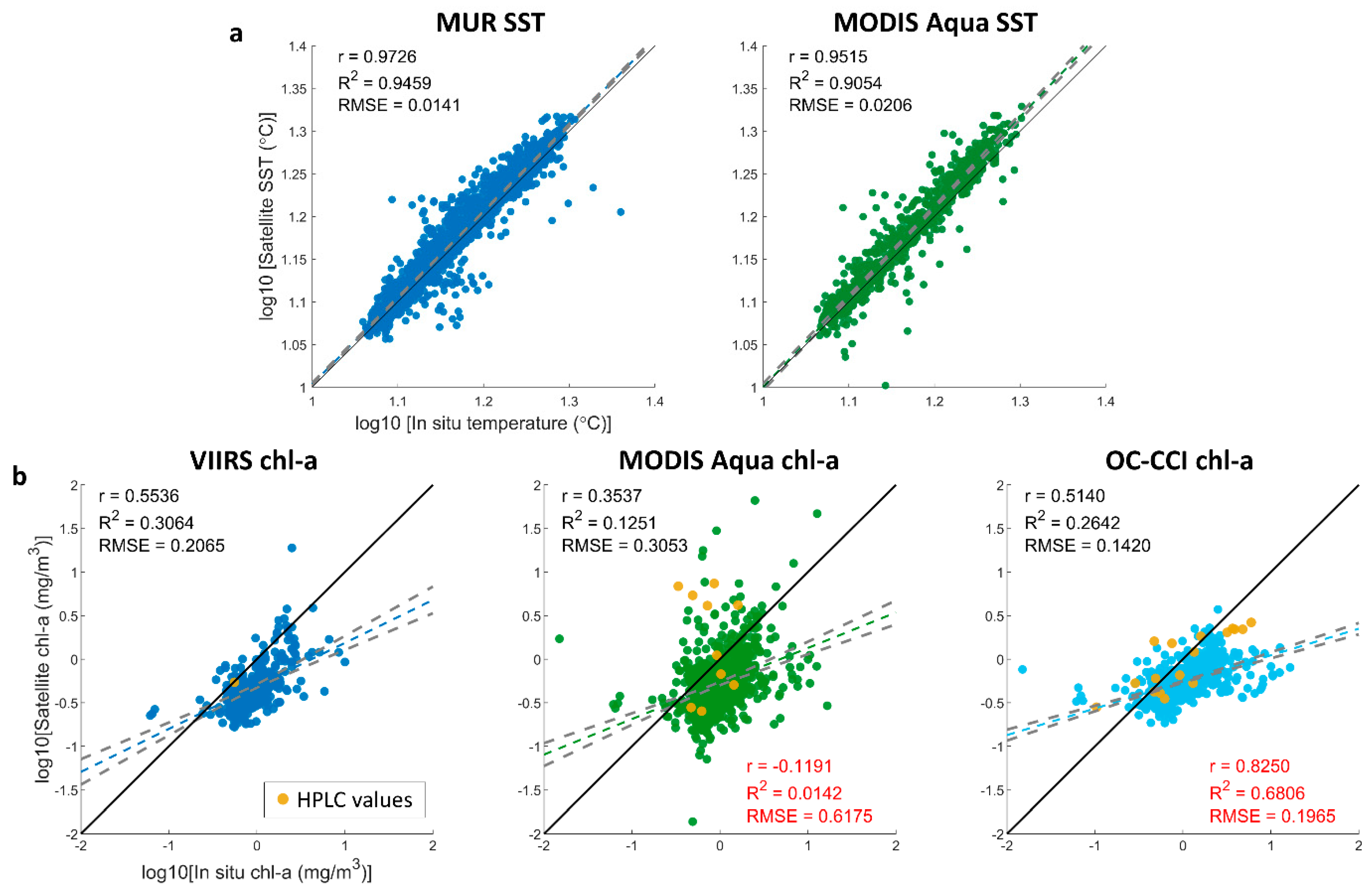
2.4. Chl-a and SST Satellite Validation

Daily 1 × 1 km v5 OC-CCI, 4 × 4 km MODIS Aqua chl-a and SST, 4 × 4 km VIIRS chl-a, and 1 × 1 km MUR SST data were used to compare to the Maria Island NRS hourly time series of chl-a and temperature taken at an approximately 20 m depth. Satellite chl-a estimates were also compared to chl-a values from the Valente et al. dataset. The Maria Island NRS data were converted to daily averages to match the satellite data temporal resolution. The nearest pixel for each sensor was matched to the Maria Island NRS and Valente et al. coordinates. Satellite chl-a and SST were plotted against in situ chl-a and temperature from the Maria Island NRS and Valente et al. data. To compare discrepancies between sensors, we analyzed chl-a time series from all MODIS Aqua, VIIRS, and OC-CCI data in the coastal study area using monthly averages to reduce temporal gaps.

3. Results

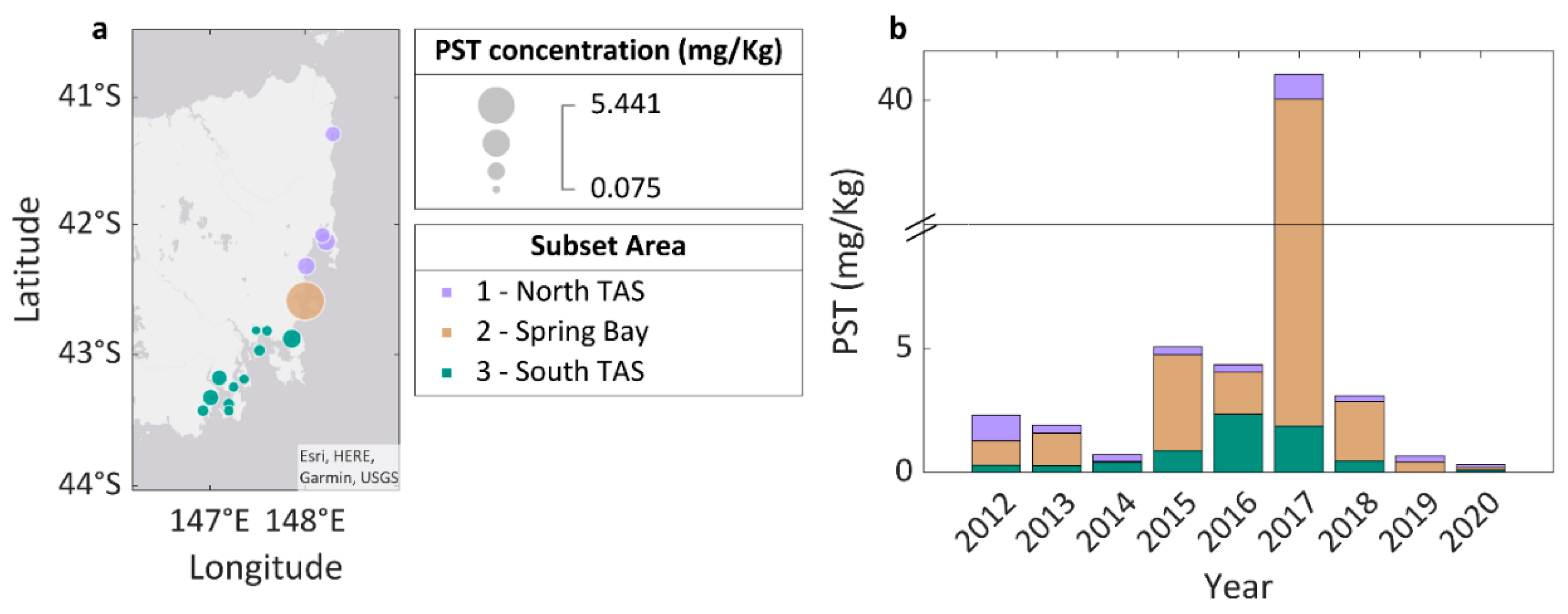
3.1. Paralytic Shellfish Toxins

The north, central (Spring Bay), and south sites all had varying toxicity levels between high PST years (Figure 2a). Spring Bay in particular had extremely high PST concentrations in 2017, with an average of 38.18 mg/kg (Figure 2b). This is over 16 times more toxic than the highest year for North TAS sites in 2016 at 2.35 mg/kg and 36 times more toxic than 2012, the highest year for South TAS, with an average of 1.04 mg/kg. The increase of PST values for North TAS first appeared in 2012 and then peaked again in 2017, while Spring Bay was more sporadic, and South TAS values slowly increased from 2012.

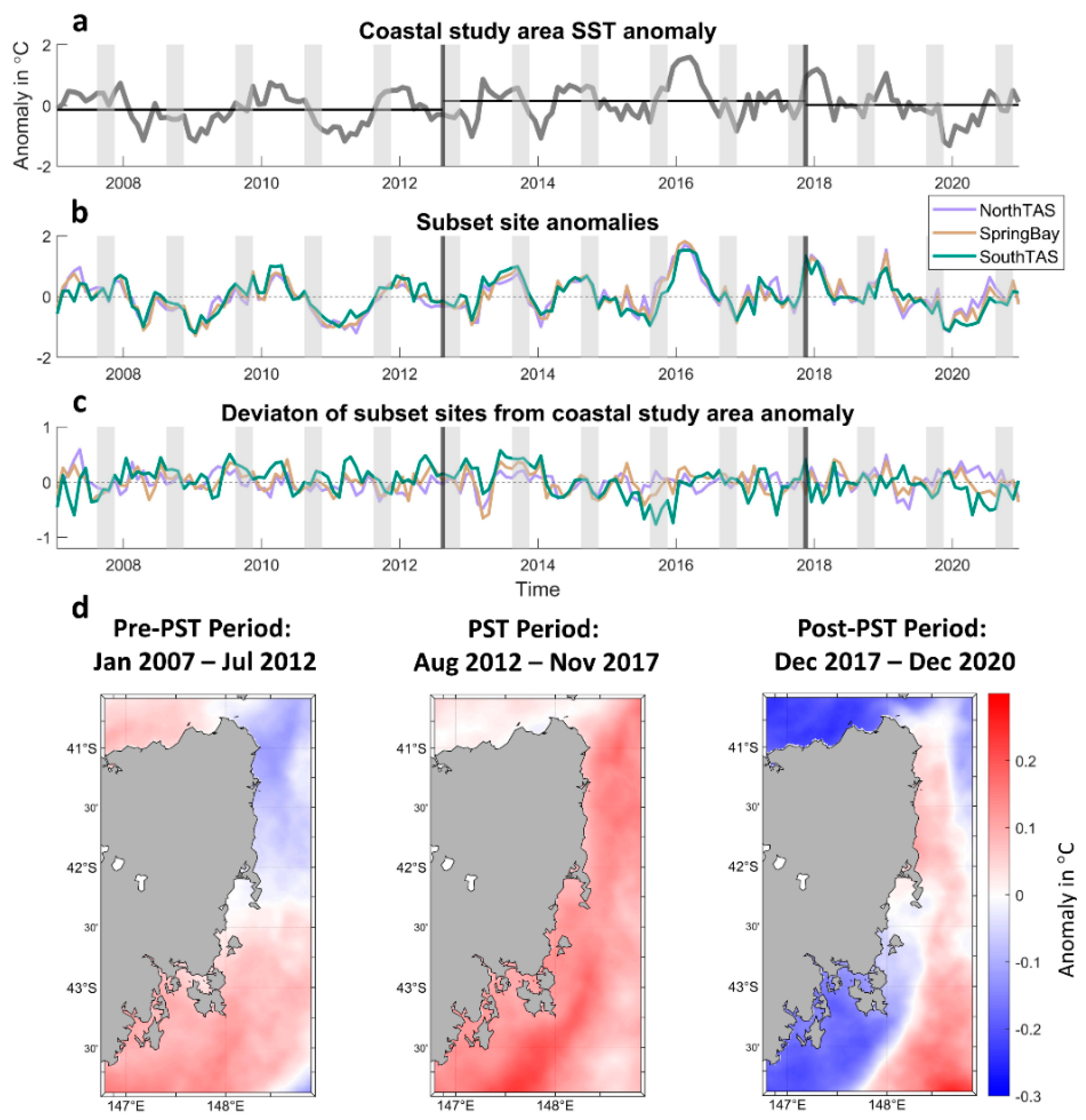
3.2. Sea Surface Temperature Spatial and Temporal Analyses

In terms of SST for the east coast shelf of Tasmania, there was a 0.52 °C increase in temperature from 2002 to 2020 for the coastal area, however using a Mann–Kendall test determined that the trend was not significant (tau = 0.0505, p = 0.261). For our time period from 2007 to 2020, there was also no significant trend (tau = −0.011, p = 0.827). When separating the time series into the pre-PST period, PST period, and post-PST period, the average PST period temperature for the coastal area was 0.29 °C warmer than the pre-PST period, and 0.16 °C warmer than the post-PST period (Figure 3a). All subset areas also showed an increase in temperature in the PST period in comparison to the pre-PST period and post-PST period, however a t-test showed that these increases were not significant between temporal periods (Figure 3b). Compared to the coastal study area, the South TAS subset area was 0.82 °C cooler during the PST period, Spring Bay was 0.38 °C cooler, and North TAS was 0.11 °C cooler (Figure 3c).
Spatially, warm anomalies occurred along the entire coast during the PST period (0.15 °C), and temporally, a positive anomaly occurred in the summer of 2015/2016 (>1.4 °C) (Figure 3d). There were cooler anomalies around the North TAS sites and warming for the South TAS in the pre-PST period. The opposite occurred in the post-PST period, with warmer anomalies in the north and cooler in the south close to the coast. There was little change for the Spring Bay pre-PST period (−0.13 °C) and post-PST period (0.003 °C).

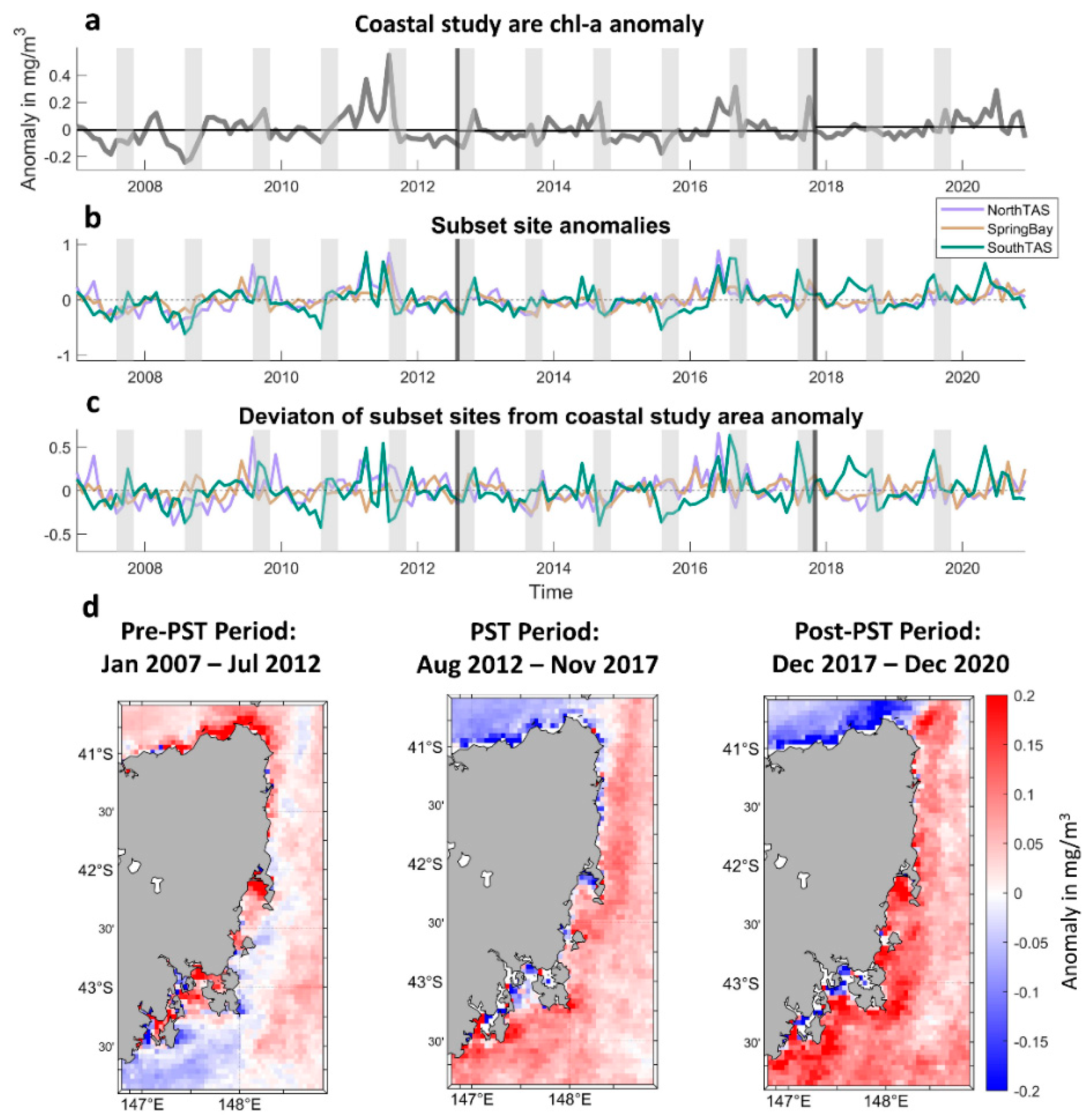
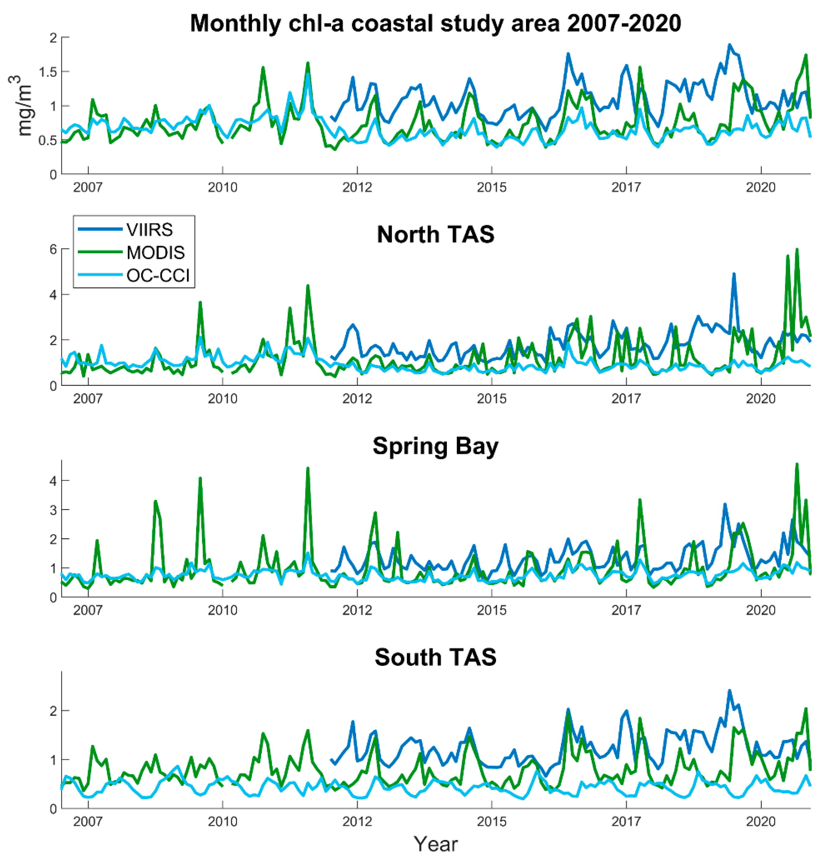
3.3. Chlorophyll-a Spatial Anomalies and Temporal Analyses

Examining all available OC-CCI chl-a data, chl-a increased by 18.5% for the coastal study area between 1997 and 2020, and using a Mann–Kendall test, there was a significant increase present (tau = 0.138, p = 6.01 × 10⁻⁴). Looking closer at our time period, chl-a showed a slight significant negative trend (tau = −0.164, p = 1.58 × 10⁻³) for the coastal study area between 2007 and 2020, with average values for the pre-PST, PST, and post-PST periods at 0.52, 0.51 (decrease of 0.5%), and 0.53 (increase of 3.3%) mg/m3, respectively (Figure 4a). Comparing the pre-PST and PST periods with a t-test, there was a significant increase in chl-a (p = 3.922 × 10⁻¹⁰), which also occurred when comparing the pre-PST and post-PST periods (p = 1.094 × 10⁻⁴). For the subset areas, North TAS chl-a increased by 5.3% during the pre-PST period to the PST period (Figure 4b). Spring Bay increased by 5.1% and South TAS also increased by 6.0%. Relative to the coastal study area, North TAS chl-a decreased by 1.2% from the pre-PST period to the PST period, Spring Bay increased by 5.9%, and South TAS also increased by 10.5% compared to the deviation values from the coastal study area (Figure 4c). There is a distinct peak in the temporal anomaly prior to the start of 2012 and then a drop during the start of the PST period. Individually, all three sites had higher chl-a concentrations during the PST period. Between the individual subset sites and the combined subset site average, North TAS chl-a dropped right before the PST period, whereas South TAS sites started to increase during the PST period and Spring Bay consistently had lower chl-a values.
As we would expect spatially due to nutrient availability and higher reflectance from suspended sediment, chl-a concentrations were over four times higher along the coast during the spring months (Figure 4d). Before the PST period, chl-a in the small bays north and south of Maria Island had stronger positive anomalies, while the south coast had a reduction in chl-a. During the PST period, there was lower chl-a directly off the coast in the smaller bays but then values increased 2–3 km off the coast. In the post-PST period, the south bays decreased in chl-a, but the rest of the coast increased, with a greater intensity than the PST period.

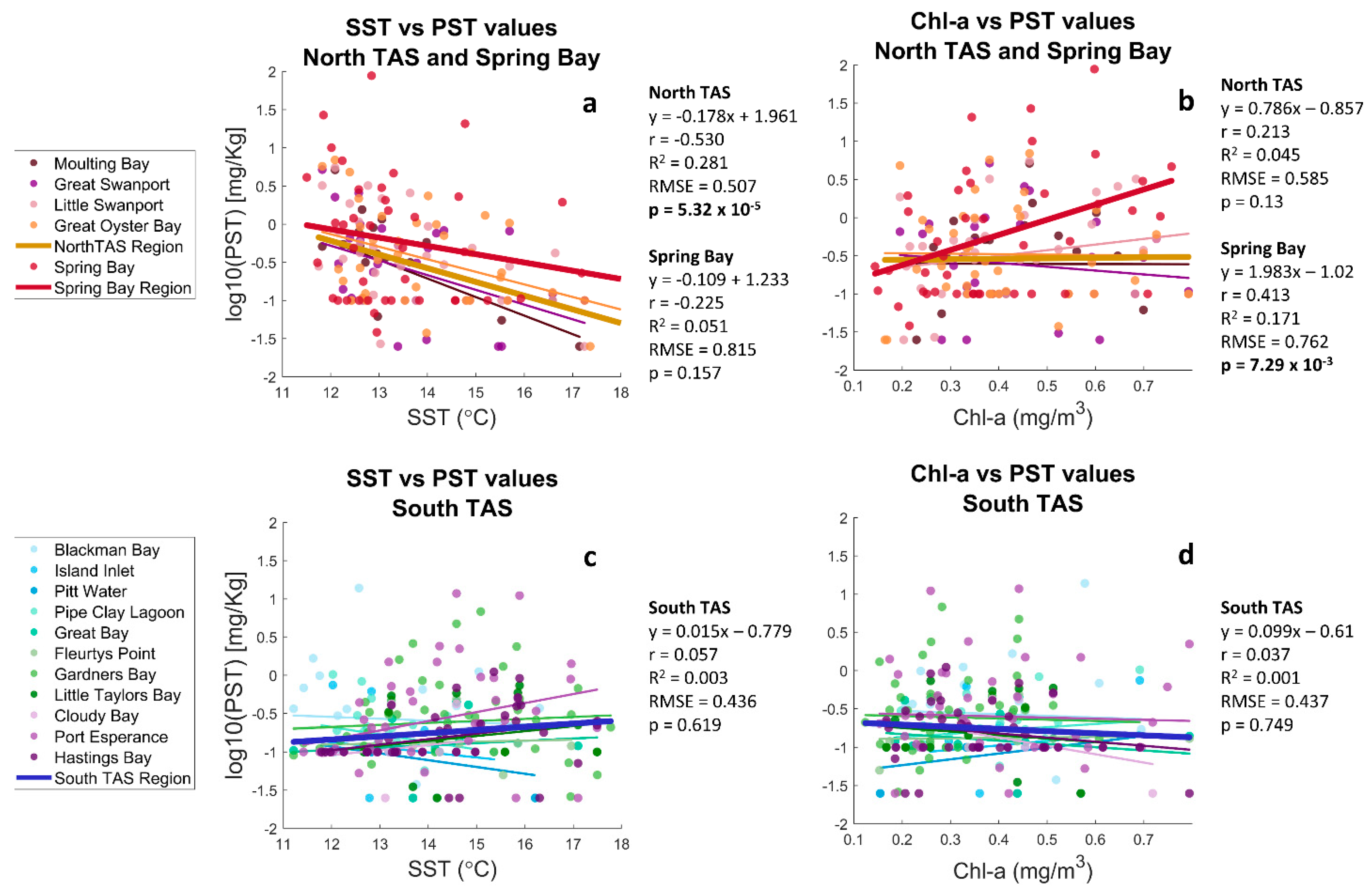
3.4. Relationships between SST, Chl-a, and Toxin Data

When comparing toxin concentration and our environmental variables, there is a distinct negative correlation between SST and PST values for the North TAS (r = −0.530, p = 5.32 × 10⁻⁵, R2 = 0.281, RMSE = 0.507) and a weak correlation for Spring Bay sites (r = −0.225, p = 0.157, R2 = 0.051, RMSE = 0.815). There are no distinct relationships between sites when comparing SST to PST for South TAS sites (r = 0.057, p = 0.619, R2 = 0.003, RMSE = 0.436). For chl-a data, Spring Bay has a positive correlation with PST values (r = 0.413, p = 0.007, R2 = 0.171, RMSE = 0.762), while all other comparisons of PST and chl-a did not show any distinct relationships (Figure 5).

3.5. Sensor Validation

Maria Island NRS temperature data from 20 m depth showed a strong match for both the MUR (r = 0.973, R2 = 0.95, r-value 95% CI = 0.971, 0.975) and MODIS Aqua SST (r = 0.952, R2 = 0.91, CI = 0.94, 0.96; Figure 6a). Chl-a for VIIRS (r = 0.55, R2 = 0.31, CI = 0.481, 0.619), MODIS Aqua (r = 0.35, R2 = 0.13, CI = 0.30, 0.41), and OC-CCI (r = 0.51, R2 = 0.26, CI = 0.47, 0.56; Figure 6b) had much lower accuracy compared to the in situ chl-a measured from a fluorescence sensor. These R2 values are very low, demonstrating the poor validation of satellite chl-a. In situ chl-a data from Valente et al.’s HPLC analyses showed the strongest relationship with OC-CCI data (r = 0.83, R2 = 0.68, CI = 0.57, 0.93), however this may be expected as the data points were used to validate OC-CCI data around Tasmania [20]. There are missing data due to clouds for the optical satellite data, so only a small number of matchups occurred with the Valente et al. dataset. There was only one matchup between the in situ HPLC analysis chl-a and the VIIRS satellite, so the r, RMSE, and R2 values could not be calculated.
For the study period between 2007 and 2020, there is high uncertainty between sensors for each of the subset areas (Figure 7). VIIRS was consistently recording higher chl-a values than MODIS Aqua until 2020. In comparison, MODIS Aqua was also recording higher values than OC-CCI for the full time period. Between 2018 and 2020, the discrepancy between sensors is the greatest (Figure 7). Overall, OC-CCI values tend to be 65.7% lower than the VIIRs and 13.4% lower than MODIS Aqua values and underestimate in situ chl-a from the Maria Island NRS fluorescence sensor by approximately 48.4% and 19.4% from the HPLC analysis data from Valente et al. for the coastal study area.

4. Discussion

One of the strongest relationships between environmental conditions and high-toxin conditions depends on temperature. However, this only pertains to the north and central coast of Tasmania, which displayed a negative correlation between temperature and PST values. For chl-a, Spring Bay showed a positive correlation with PST values, but the coastal study area and other subset areas did not illustrate any clear relationships spatially or temporally between 2007 and 2020. Xie et al.’s study emphasized low temperatures and high chl-a in relation to PST values for the east coast study area, which matched with our temperature analysis and the Spring Bay chl-a [4].
More specifically, our results displayed anomalously high SST along the coast during the high PST period, however for the North TAS and Spring Bay sites, SST correlated negatively with PST. The conditions for A. catenella growth and bloom development may be better in cooler waters of 10–15 °C for Tasmania and high toxin production has been shown to have an inverse relationship with temperature, but this may be dependent on specific strains [1,20,21]. One study in the Bay of Fundy showed increased toxicity at temperatures lower than 10 °C but also showed an increase at the highest experimental temperatures (25 °C) [22]. This implies that the increased PST values during the warm coastal anomaly could be due to stress of the high temperature increases, or an increase in predators [9,21].
The increase of toxins based on the grazing pressure from zooplankton is a possibility as increases in ocean temperatures since 2009 have also led to an increase in zooplankton numbers on the southeast coast of Tasmania, and a spike in 2015/2016 during a marine heatwave due to the extension of the EAC [5,10,12,13,14]. The maximum abundance recorded was in January of 2017 for the southeast coast. Due to the lack of zooplankton data on the central and north east coast during in 2017, it remains difficult to determine if the increases occurred in the Spring Bay and North TAS sites as well, or if the high abundances continued into spring, which was the highest year for PST values for the north and central sites [13]. The Spring Bay site displayed a positive correlation between chl-a values from satellite data and PST values. This also supports the grazing-toxin production hypothesis as the increase in phytoplankton biomass may increase predator presence with an increase in its food source [13].
To develop an understanding of biomass changes and the community composition, chl-a data can be separated into phytoplankton functional types (PFTs) or class sizes based on pigments [23,24]. Specifically, Hirata et al. derive dinoflagellate and diatom estimates from chl-a data, where the ratio of diatom:dinoflagellate abundance is positively related to chlorophyll concentration [24,25]. For southeast Australia, the total phytoplankton abundance collected from in situ datasets were predominantly diatoms for 1965–2015, and the Hirata et al. algorithm estimated that 98% of the chl-a off the east coasts of Tasmania consisted of diatoms [25]. On the southeast coast of Tasmania, the ratio of diatom:dinoflagellate at the Maria Island NRS was the highest during the spring and summer months from 1997 to 2007 [11]. Our results showed a decrease of chl-a for the coastal study area during the PST period, which we would expect if there was a decrease in the diatom:dinoflagellate ratio or a decrease in diatoms in general.
It was concluded that during the PST period in Tasmania, even small abundances of Alexandrium cells, 50–100 cells/L, were linked to high PST concentrations between 2012 and 2017 [1]. These dynamics of the low cell counts and high toxin concentrations should be researched further and Alexandrium abundance should be distinguished at a species level to determine if environmental conditions, ecosystem dynamics, or an increased abundance of A. catenella has a larger influence on toxin production. In regard to remote sensing, small quantities of dinoflagellates can be difficult to analyze through satellite chl-a data, especially if there are discrepancies with chl-a data; however, chlorophyll levels may be useful to diagnose the broader environmental conditions that lead to PST events.
A major concern of using chl-a data to compare toxin events or HABs to chl-a satellite values are the weak matchups with the in situ data from all three sensors and the limited spatial coverage of in situ data. There were large differences between the chl-a sensors, and the OC-CCI and VIIRS products underestimated chl-a compared to the Maria Island NRS data for the coastal study area and subset areas. This could be due to the fact that in situ samples were taken at a 20 m depth rather than the surface, as well as the measurements coming from a fluorescence sensor rather than HPLC analysis [26,27]. However, chl-a data from the Valente et al. HPLC analysis also showed weak matchups with OC-CCI, while MODIS Aqua data and SST values from the blended MUR dataset and MODIS both show strong matchups to the station data, even with the in situ data recorded at 20 m depth. The mixed-layer depth around the southeast coast of Tasmania fluctuates between 5 and 30 m, so the Maria Island NRS sensor potentially collects values in this range [28,29,30]. Additionally, east coast Tasmania freshwater inputs from rivers make it a complex area and difficult to use optical sensor chl-a measurements as tannins from rivers mix with coastal waters. This uncertainty between sensors and the in situ chl-a implies the need for the development of a localized chl-a algorithm for optical sensors [31].
Improvements in satellite detection, regional chl-a algorithms, the understanding of local dynamics, and additional in situ data collection will help in the analysis of environmental conditions around Tasmania. The Plankton, Aerosol, Cloud, ocean Ecosystem (PACE) project will help with large-scale detection, collecting high-resolution data in the ultraviolet spectral band, recently shown to distinguish blooms of the dinoflagellate Lingulodinium polyedra. Other products including chl-a, net primary production, phytoplankton pigment concentrations, and spectral phytoplankton absorption coefficients will help measure biomass and decipher phytoplankton groups and species from one another [32,33]. The PACE satellite may be able to distinguish the spectral signature of Alexandrium around Tasmania, helping to detect and monitor the spatial extent [32]. Local algorithms can also help improve chl-a estimation along the coast of Tasmania, along with high-resolution models to be able to look at local environmental conditions of smaller bays and coastal areas where the high PST values occurred. Along with sensor and algorithm development, the addition of chl-a measurements from HPLC analysis for the whole east coast of Tasmania would be useful to distinguish whether there is a strong relationship with high PST concentrations. Additionally, the collection of zooplankton abundance and phytoplankton cell counts at a species level can help with PST predictions and determine if the toxins are driven by environmental conditions, A. catenella abundance increases, or are a response to predator presence [34].

5. Conclusions

Our study sought to establish the environmental context for PST events in eastern coastal Tasmania using remote sensing. We showed negative relationships between sea surface temperature for the north and central sites, and no strong relationships between PST and the remote-sensed environmental conditions for the south coast sites. The hypotheses of increased PST with increased SST and decreased chl-a cannot be fully supported by this study alone due to a lack of in situ chl-a, zooplankton, and toxic phytoplankton data. However, the examination of spatial and temporal trends for the east coast of Tasmania is important to determine how open-ocean and coastal areas may be changing over time and if similar conditions for high PST events may appear again. All chl-a satellite data showed weak matchups with chl-a recorded from the Maria Island NRS and the Valente et al. dataset, which may be due to the sampling depth at 20 m or inaccuracies in the satellite estimates. The analysis of chl-a satellite and in situ data for a localized area helps to distinguish uncertainties in remote sensing data for coastal areas and highlights the need for region-specific algorithms. To further test the hypotheses concerning the relationship between PST and chl-a, continuous sampling for toxins and toxic phytoplankton counts at a species level, combined with zooplankton data, should be implemented on the east coast of Tasmania. In addition, improved satellite products and meteorological data, such as ocean currents, wind, rainfall, and river flow, will help us to better understand the environmental drivers of HABs and build predictive models.

Author Contributions

Conceptualization, A.M.F.; Methodology, G.L.B. and A.M.F.; Formal Analysis, L.W., E.J.S. and G.L.B.; Writing—Original Draft Preparation, L.W.; Writing—Review and Editing, L.W., G.L.B., E.J.S. and A.M.F.; Visualization, L.W., E.J.S. and G.L.B.; Supervision, G.L.B. and A.M.F.; Funding Acquisition, A.M.F. All authors have read and agreed to the published version of the manuscript.

Funding

This research was supported by the Institute for Marine and Antarctic Studies at the University of Tasmania for L.W. and A.M.F. Funding was also provided by the Simons Foundation Postdoctoral Fellowship in Marine Microbial Ecology (Grant # 645921) for G.L.B.

Data Availability Statement

Restrictions apply to the availability of ShellMAP paralytic shellfish toxin data. Data were obtained from ShellMAP and are available with permission. The rest of the data presented in this study are openly available. JPL MUR MEaSUREs Project. 2015. GHRSST Level 4 MUR Global Foundation Sea Surface Temperature Analysis. Ver. 4.1. PO.DAAC, CA, USA. https://doi.org/https://doi.org/10.5067/GHGMR-4FJ04 Accessed 26 April 2021. Color Climate Change Initiative (Ocean_Color_CCI). Sathyendranath, S.; Jackson, T.; Brockmann, C.; Brotas, V.; Calton, B.; Chuprin, A.; Clements, O.; Cipollini, P.; Danne, O.; Dingle, J.; Donlon, C.; Grant, M.; Groom, S.; Krasemann, H.; Lavender, S.; Mazeran, C.; Mélin, F.; Müller, D.; Steinmetz, F.; Valente, A.; Zühlke, M.; Feldman, G.; Franz, B.; Frouin, R.; Werdell, J.; Platt, T. 2021. ESA Ocean. Version 5.0 Data. NERC EDS Centre for Environmental Data Analysis. http://dx.doi.org/10.5285/1dbe7a109c0244aaad713e078fd3059a Accessed 26 April 2021. Moderate-Resolution Imaging Spectroradiometer (MODIS) Aqua Chlorophyll Data. NASA Goddard Space Flight Center, Ocean Ecology Laboratory, Ocean Biology Processing Group. 2018 Reprocessing. NASA OB.DAAC, Greenbelt, MD, USA. Version 2018.0. https://doi.org/data/10.5067/AQUA/MODIS/L3M/CHL/2018 Accessed 18 October 2021. Visible and Infrared Imager/Radiometer Suite (VIIRS) Chlorophyll Data. NASA Goddard Space Flight Center, Ocean Ecology Laboratory, Ocean Biology Processing Group. 2018 Reprocessing. NASA OB.DAAC, Greenbelt, MD, USA. https://doi.org/data/10.5067/NPP/VIIRS/L3M/CHL/2018 Accessed 18 October 2021. Integrated Marine Observing System (IMOS) in situ chlorophyll data. 2009. IMOS—ANMN National Reference Station (NRS) Maria Island Mooring. https://portal.aodn.org.au/search?uuid=7b901002-b1dc-46c3-89f2-b4951cedca48 Accessed 9 October 2021. OC-CCI in situ database: Valente, A.; Sathyendranath, S.; Brotas, V.; Groom, S.; Grant, M.; Taberner, M.; Antoine, D.; Arnone, R.; Balch, W.M.; Barker, K.; Barlow, R.; Bélanger, S.; Berthon, J.-F.; Besiktepe, S.; Borsheim, Y.; Bracher, A.; Brando, V.; Canuti, E.; Chavez, F.; Cianca, A.; Claustre, H.; Clementson, L.; Crout, R.; Frouin, R.; García-Soto, C.; Gibb, S.W.; Gould, R.; Hooker, S.B.; Kahru, M.; Kampel, M.; Klein, H.; Kratzer, S.; Kudela, R.; Ledesma, J.; Loisel, H.; Matrai, P.; McKee, D.; Mitchell, B.G.; Moisan, T.; Muller-Karger, F.; O’Dowd, L.; Ondrusek, M.; Platt, T.; Poulton, A.J.; Repecaud, M.; Schroeder, T.; Smyth, T.; Smythe-Wright, D.; Sosik, H.M.; Twardowski, M.; Vellucci, V.; Voss, K.; Werdell, J.; Wernand, M.; Wright, S.; Zibordi, G. 2019. A compilation of global bio-optical in situ data for ocean-color satellite applications—Version two. Earth Syst. Sci. Data 11, 1037–1068. https://doi.org/10.5194/essd-11-1037-2019 Accessed 18 October 2021.

Acknowledgments

We would like to thank Christopher Bolch and Gustaaf Hallegraeff for the valuable discussions regarding phytoplankton phenology and harmful algal blooms, as well as Christina Schallenberg and Pete Strutton for the very helpful meetings on the manuscript structure and analysis suggestions. We would like to acknowledge NASA, OC-CCI, and Australia’s IMOS for distributing their data. IMOS is enabled by the National Collaborative Research Infrastructure Strategy (NCRIS). It is operated by a consortium of institutions as an unincorporated joint venture, with the University of Tasmania as Lead Agent. We would like to acknowledge the Shellfish Market Access Program (ShellMAP) for the paralytic shellfish toxin data and helpful conversations regarding the data. Thank you to the reviewers for the constructive comments to help improve this manuscript. This work was supported by the University of Tasmania, Institute for Marine and Antarctic Studies and the Simons Foundation.

Conflicts of Interest

The authors declare no conflict of interest.

References

  1. Hallegraeff, G.M.; Bolch, C.; Campbell, K.; Condie, S.; Dorantes-Aranda, J.; Murray, S.; Turnbull, A.; Ugalde, S. Improved Understanding of Tasmanian Harmful Algal Blooms and Biotoxin Events to Support Seafood Risk Management; Fisheries Research and Development Corporation: Deakin, ACT, Australia, 2018; ISBN 1925646084. [Google Scholar]
  2. Condie, S.A.; Oliver, E.C.J.; Hallegraeff, G.M. Environmental drivers of unprecedented Alexandrium catenella dinoflagellate blooms off eastern Tasmania, 2012–2018. Harmful Algae 2019, 87, 101628. [Google Scholar] [CrossRef] [PubMed]
  3. Hallegraeff, G.M.; Schweibold, L.; Jaffrezic, E.; Rhodes, L.; MacKenzie, L.; Hay, B.; Farrell, H. Overview of Australian and New Zealand harmful algal species occurrences and their societal impacts in the period 1985 to 2018, including a compilation of historic records. Harmful Algae 2020, 102, 101848. [Google Scholar] [CrossRef] [PubMed]
  4. Xie, H.; Fischer, A.M.; Strutton, P.G. Generalized linear models to assess environmental drivers of paralytic shellfish toxin blooms (Southeast Tasmania, Australia). Cont. Shelf Res. 2021, 223, 104439. [Google Scholar] [CrossRef]
  5. Oliver, E.C.J.; Lago, V.; Hobday, A.J.; Holbrook, N.J.; Ling, S.D.; Mundy, C.N. Marine heatwaves off eastern Tasmania: Trends, interannual variability, and predictability. Prog. Oceanogr. 2018, 161, 116–130. [Google Scholar] [CrossRef]
  6. Grebner, W.; Berglund, E.C.; Berggren, F.; Eklund, J.; Harðadóttir, S.; Andersson, M.X.; Selander, E. Induction of defensive traits in marine plankton—New copepodamide structures. Limnol. Oceanogr. 2019, 64, 820–831. [Google Scholar] [CrossRef]
  7. Lundholm, N.; Krock, B.; John, U.; Skov, J.; Cheng, J.; Pančić, M.; Wohlrab, S.; Rigby, K.; Nielsen, T.G.; Selander, E.; et al. Induction of domoic acid production in diatoms—Types of grazers and diatoms are important. Harmful Algae 2018, 79, 64–73. [Google Scholar] [CrossRef] [PubMed]
  8. Selander, E.; Thor, P.; Toth, G.; Pavia, H. Copepods induce paralytic shellfish toxin production in marine dinoflagellates. Proc. R. Soc. B Biol. Sci. 2006, 273, 1673–1680. [Google Scholar] [CrossRef] [PubMed] [Green Version]
  9. Selander, E.; Fagerberg, T.; Wohlrab, S.; Pavia, H. Fight and flight in dinoflagellates? Kinetics of simultaneous grazer-induced responses in Alexandrium tamarense. Limnol. Oceanogr. 2011, 57, 58–64. [Google Scholar] [CrossRef]
  10. Kelly, P.; Clementson, L.; Davies, C.; Corney, S.; Swadling, K. Zooplankton responses to increasing sea surface temperatures in the southeastern Australia global marine hotspot. Estuar. Coast. Shelf Sci. 2016, 180, 242–257. [Google Scholar] [CrossRef]
  11. Thompson, P.A.; Baird, M.E.; Ingleton, T.; Doblin, M.A. Long-term changes in temperate Australian coastal waters: Implications for phytoplankton. Mar. Ecol. Prog. Ser. 2009, 394, 1–19. [Google Scholar] [CrossRef] [Green Version]
  12. Thompson, P.A.; Bonham, P.; Thomson, P.; Rochester, W.; Doblin, M.A.; Waite, A.M.; Richardson, A.; Rousseaux, C.S. Climate variability drives plankton community composition changes: The 2010–2011 El Niño to La Niña transition around Australia. J. Plankton Res. 2015, 37, 966–984. [Google Scholar] [CrossRef] [Green Version]
  13. Evans, R.; Lea, M.A.; Hindell, M.A.; Swadling, K.M. Significant shifts in coastal zooplankton populations through the 2015/16 Tasman Sea marine heatwave. Estuar. Coast. Shelf Sci. 2020, 235, 106538. [Google Scholar] [CrossRef]
  14. Oliver, E.C.J.; Benthuysen, J.A.; Bindoff, N.L.; Hobday, A.J.; Holbrook, N.J.; Mundy, C.N.; Perkins-Kirkpatrick, S.E. Theunprecedented 2015/16 Tasman Sea marine heatwave. Nat. Commun. 2017, 8, 16101. [Google Scholar] [CrossRef] [PubMed] [Green Version]
  15. Sathyendranath, S.; Brewin, B.; Mueller, D.; Doerffer, R.; Krasemann, H.; Melin, F.; Brockmann, C.; Fomferra, N.; Peters, M.; Grant, M.; et al. Ocean Colour Climate Change Initiative—Approach and initial results. Int. Geosci. Remote Sens. Symp. 2012, 2024–2027. [Google Scholar] [CrossRef]
  16. Chin, T.M.; Vazquez-cuervo, J.; Armstrong, E.M. Remote Sensing of Environment A multi-scale high-resolution analysis of global sea surface temperature. Remote Sens. Environ. 2017, 200, 154–169. [Google Scholar] [CrossRef]
  17. Davies, C.; Sommerville, E.; Hidas, M.; Suthers, I.; Lara-Lopez, A.; Matis, P.; Van Derk Kamp, J.; Tibben, S.; Abell, G.; Allen, S.; et al. National Reference Stations Biogeochemical Operations Manual—Version 3.3.1; Integrated Marine Observing System: Hobart, Australia, 2020. [Google Scholar]
  18. Burgoyne, M.; Mills, A. Tasmanian Shellfish Market Access Program (ShellMAP) Biotoxin Management Plan Version 5.1; Department of Primary Industries, Parks, Water and Environment, Tasmanian Government: Hobart, Australia, 2019. [Google Scholar]
  19. Krasemann, H.; Müller, D.; Mélin, F.; Valente, A.; Grant, M. Product Validation and Inter-Comparison Report; Plymouth Marine Laboratory: Plymouth, UK, 2017. [Google Scholar]
  20. Aguilera-Belmonte, A.; Inostroza, I.; Franco, J.M.; Riobó, P.; Gómez, P.I. The growth, toxicity and genetic characterization of seven strains of Alexandrium catenella (Whedon and Kofoid) Balech 1985 (Dinophyceae) isolated during the 2009 summer outbreak in southern Chile. Harmful Algae 2011, 12, 105–112. [Google Scholar] [CrossRef]
  21. Navarro, J.M.; Muñoz, M.G.; Contreras, A.M. Temperature as a factor regulating growth and toxin content in the dinoflagellate Alexandrium catenella. Harmful Algae 2006, 5, 762–769. [Google Scholar] [CrossRef]
  22. Etheridge, S.M.; Roesler, C.S. Effects of temperature, irradiance, and salinity on photosynthesis, growth rates, total toxicity, and toxin composition for Alexandrium fundyense isolates from the Gulf of Maine and Bay of Fundy. Deep Sea Res. Part II Top. Stud. Oceanogr. 2005, 52, 2491–2500. [Google Scholar] [CrossRef]
  23. Bracher, A.; Bouman, H.A.; Brewin, R.J.W.; Bricaud, A.; Brotas, V.; Ciotti, A.M.; Clementson, L.; Devred, E.; Di Cicco, A.; Dutkiewicz, S.; et al. Obtaining phytoplankton diversity from ocean color: A scientific roadmap for future development. Front. Mar. Sci. 2017, 4, 55. [Google Scholar] [CrossRef] [Green Version]
  24. Hirata, T.; Hardman-Mountford, N.J.; Brewin, R.J.W.; Aiken, J.; Barlow, R.; Suzuki, K.; Isada, T.; Howell, E.; Hashioka, T.; Noguchi-Aita, M.; et al. Synoptic relationships between surface Chlorophyll-a and diagnostic pigments specific to phytoplankton functional types. Biogeosciences 2011, 8, 311–327. [Google Scholar] [CrossRef] [Green Version]
  25. Ajani, P.A.; Hallegraeff, G.M.; Allen, D.; Coughlan, A.; Richardson, A.J.; Armand, L.K.; Ingleton, T.; Murray, S.A. Establishing Baselines: Eighty Years of Phytoplankton Diversity and Biomass in South-Eastern Australia. Oceanogr. Mar. Biol. Annu. Rev. 2016, 54, 395–420. [Google Scholar] [CrossRef]
  26. Smith, R.C. Remote Sensing and Depth Distribution of Ocean Chlorophyll on JSTOR. Mar. Ecol. Prog. Ser. 1981, 5, 359–361. [Google Scholar] [CrossRef]
  27. Chekalyuk, A.; Hafez, M. Photo-physiological variability in phytoplankton chlorophyll fluorescence and assessment of chlorophyll concentration. Opt. Express 2011, 19, 22643. [Google Scholar] [CrossRef] [PubMed]
  28. Herraiz-Borreguero, L.; Rintoul, S.R. Regional circulation and its impact on upper ocean variability south of Tasmania. Deep. Res. Part II Top. Stud. Oceanogr. 2011, 58, 2071–2081. [Google Scholar] [CrossRef]
  29. Westwood, K.J.; Brian Griffiths, F.; Webb, J.P.; Wright, S.W. Primary production in the Sub-Antarctic and Polar Frontal Zones south of Tasmania, Australia; SAZ-Sense survey, 2007. Deep Sea Res. Part II Top. Stud. Oceanogr. 2011, 58, 2162–2178. [Google Scholar] [CrossRef] [Green Version]
  30. Herzfeld, M.; Andrewartha, J.; Sakov, P. Modelling the physical oceanography of the D’Entrecasteaux Channel and the Huon Estuary, south-eastern Tasmania. Mar. Freshw. Res. 2010, 61, 568–586. [Google Scholar] [CrossRef]
  31. Cherukuru, N.; Brando, V.E.; Schroeder, T.; Clementson, L.A.; Dekker, A.G. Influence of river discharge and ocean currents on coastal optical properties. Cont. Shelf Res. 2014, 84, 188–203. [Google Scholar] [CrossRef]
  32. Kahru, M.; Anderson, C.; Barton, A.D.; Carter, M.L.; Catlett, D.; Send, U.; Sosik, H.M.; Weiss, E.L.; Mitchell, B.G. Satellite detection of dinoflagellate blooms off California by UV reflectance ratios. Elem. Sci. Anthr. 2021, 9, 00157. [Google Scholar] [CrossRef]
  33. Werdell, P.J.; Behrenfeld, M.J.; Bontempi, P.S.; Boss, E.; Cairns, B.; Davis, G.T.; Franz, B.A.; Gliese, U.B.; Gorman, E.T.; Hasekamp, O.; et al. The Plankton, Aerosol, Cloud, Ocean Ecosystem Mission: Status, Science, Advances. Bull. Am. Meteorol. Soc. 2019, 100, 1775–1794. [Google Scholar] [CrossRef]
  34. Trapp, A.; Heuschele, J.; Selander, E. Eavesdropping on plankton—Can zooplankton monitoring improve forecasting of biotoxins from harmful algae blooms? Limnol. Oceanogr. 2021, 66, 3455–3471. [Google Scholar] [CrossRef]
Figure 1. The east coast of Tasmania study area. The broader coastal study area is defined by a gray bounding box, where satellite data values in the area are spatially averaged. This coastal area is also subset into the North TAS, Spring Bay, and South TAS areas to examine local conditions. The Maria Island NRS station, where chl-a data were collected, is represented by a green circle. The marine farms, where toxin data were collected, are shown as yellow triangles.
Remotesensing 14 00665 g001
Figure 2. Intensity map of the average PST values for the east coast from 2012 to 2020 (a). Average PST values for each year categorized by North TAS, Spring Bay, and South TAS (b). PST values are measured in shellfish tissue and the intensity map shows the location of the marine farm sites. Note the discontinuous vertical axis scale to accommodate the anomalously high toxin levels in 2017.
Remotesensing 14 00665 g002
Figure 3. Time series and spatial maps for SST split into periods of before, during, and after high PST years. Top panels (a) present the anomaly time series for the coastal area and the average of each period is displayed with a horizontal black line. Panel (b) presents the time series anomalies for each study area. Panel (c) presents the time series anomalies calculated for each study site relative to the coastal area. Panel (d) presents the average temperature anomaly for the PST event months within each time period. Pre–PST period, PST period, and post–PST period time periods are separated by vertical black lines. PST event months (August–November) are indicated with vertical light-grey shading for each year.
Remotesensing 14 00665 g003
Figure 4. Time series and spatial maps for chl-a split into periods of before, during, and after high PST years. Top panels (a) present the anomaly time series for the coastal area and the average of each period is displayed by a horizontal black line. Panel (b) presents the time series anomalies for each study area. Panel (c) presents the time series anomalies calculated for each study site relative to the coastal area. Panel (d) presents the average chl-a anomaly for the PST event months within each time period. Pre–PST period, PST period, and post–PST period time periods are separated by vertical black lines. PST event months (August–November) are indicated with vertical light-grey shading for each year.
Remotesensing 14 00665 g004
Figure 5. The comparison of PST values to environmental data from all marine farms in 2012–2020. SST vs. PST data and chl-a vs. PST data for North TAS combined with Spring Bay (a,b) and South TAS (c,d) are shown along with linear regression lines (thick). Additional regression lines (thin) shown are from the individual marine farms and correspond to the scatter point color.
Remotesensing 14 00665 g005
Figure 6. Validation of SST measurements from MUR and MODIS Aqua in comparison to in situ temperature data from the Maria Island NRS against MUR and MODIS Aqua SST (a). The 1:1 line is represented as a solid black line and the gray dashed lines represent the 95% confidence interval. Correlation coefficient (r), R2, and RMSE values comparing the temperature or chl-a from Maria Island NRS are shown in black in the top-left corner of each plot. Validation of in situ chl-a from the Maria Island NRS and the Valente et al. HPLC analysis against VIIRS, MODIS Aqua, and OC–CCI chl-a (b). Values from the HPLC analysis are shown in yellow and their r, R2, and RMSE for the datasets are shown in red in the bottom-right of each plot.
Remotesensing 14 00665 g006
Figure 7. Monthly chl-a time series for each sensor: VIIRS, MODIS Aqua, and OC–CCI, and the subset areas.
Remotesensing 14 00665 g007
Table 1. Subset categories and the marine farms included in each subset.
CategoryNorth TASSpring BaySouth TAS
Marine FarmsMoulting Bay, Great Swanport, Little Swanport, Great Oyster BaySpring BayBlackman Bay, Pitt Water, Island Inlet, Pipe Clay Lagoon, Great Bay, Fleurty’s Point, Gardner’s Bay, Little Taylor’s Bay, Cloudy Bay, Port Esperance, Hastings Bay
Total4111
Publisher’s Note: MDPI stays neutral with regard to jurisdictional claims in published maps and institutional affiliations.

