
Lite-YOLOv5: A Lightweight Deep Learning Detector for On-Board Ship Detection in Large-Scene Sentinel-1 SAR Images


School of Information and Communication Engineering, University of Electronic Science and Technology of China, Chengdu 611731, China
*
Author to whom correspondence should be addressed.
Remote Sens. 2022, 14(4), 1018; https://doi.org/10.3390/rs14041018
Submission received: 30 December 2021
/
Revised: 6 February 2022
/
Accepted: 7 February 2022
/
Published: 20 February 2022
(This article belongs to the Special Issue Artificial Intelligence-Based Learning Approaches for Remote Sensing)
Abstract
:Synthetic aperture radar (SAR) satellites can provide microwave remote sensing images without weather and light constraints, so they are widely applied in the maritime monitoring field. Current SAR ship detection methods based on deep learning (DL) are difficult to deploy on satellites, because these methods usually have complex models and huge calculations. To solve this problem, based on the You Only Look Once version 5 (YOLOv5) algorithm, we propose a lightweight on-board SAR ship detector called Lite-YOLOv5, which (1) reduces the model volume; (2) decreases the floating-point operations (FLOPs); and (3) realizes the on-board ship detection without sacrificing accuracy. First, in order to obtain a lightweight network, we design a lightweight cross stage partial (L-CSP) module to reduce the amount of calculation and we apply network pruning for a more compact detector. Then, in order to ensure the excellent detection performance, we integrate a histogram-based pure backgrounds classification (HPBC) module, a shape distance clustering (SDC) module, a channel and spatial attention (CSA) module, and a hybrid spatial pyramid pooling (H-SPP) module to improve detection performance. To evaluate the on-board SAR ship detection ability of Lite-YOLOv5, we also transplant it to the embedded platform NVIDIA Jetson TX2. Experimental results on the Large-Scale SAR Ship Detection Dataset-v1.0 (LS-SSDD-v1.0) show that Lite-YOLOv5 can realize lightweight architecture with a 2.38 M model volume (14.18% of model size of YOLOv5), on-board ship detection with a low computation cost (26.59% of FLOPs of YOLOv5), and superior detection accuracy (1.51% F1 improvement compared with YOLOv5).
1. Introduction
In recent years, an increasing number of high-quality microwave remote sensing images have been provided by synthetic aperture radar (SAR) satellites. Due to the all-day and all-weather ability of SAR, SAR remote sensing images have been widely applied in the field of ship detection. Currently, increasing number of scholars are paying attention to ship detection in SAR images due to its potential application in environmental monitoring, shipwreck rescue, oil leakage detection, marine shipping control [1,2,3,4], etc. Thus, it is of great significance to obtain the real-time and accurate ship detection results.
Recently, there have been great breakthroughs of deep learning (DL) in several fields, including computer vision (CV), natural language processing (NLP), communications, and networking [5,6]. An increasing amount of attention has been focused on SAR-based processing based on convolutional neural networks (CNNs) [7,8], especially for ship detection in SAR images. For example, Kang et al. [9] utilized contextual region-based CNN based on multilayer fusion in the field of SAR ship detection. Jiao et al. [10] proposed a densely connected end-to-end neural network to solve the problem of multi-scale and multi-scene SAR ship detection. Cui et al. [11] used a dense attention pyramid network (DAPN) for multi-scene SAR ship detection, where a pyramid structure and convolutional block attention module were adopted. Liu et al. [12] used multi-scale proposal generation for SAR ship detection, with a framework that mainly contained hierarchical grouping and proposal scoring. Wang et al. [13] proposed a rotatable bounding box ship detection method fused with an attention module and angle regression. An et al. [14] proposed an improved rotatable bounding box SAR ship detection framework, where a feature pyramid network (FPN), a modified encoding scheme, and a focal loss (FL) combined with hard negative mining (HNM) technique were adopted. Chen et al. [15] proposed a ship detection network combined with an attention module which can accurately locate ships in complex scenes. Dai et al. [16] proposed a novel CNN for multi-scale SAR ship detection, which is composed of a fusion feature extraction network (FFEN), a region proposal network (RPN), and a refined detection network (RDN). Wei et al. [17] offered a precise and robust ship detector based on a high-resolution ship detection network (HR-SDNet). The above methods have achieved fairish performance in the SAR ship detection field. However, they all have complex models and huge calculations, which can be a significant obstacle to deploy on satellites with limited memory and computation resources for on-board detection. The issue of obtaining high model detection performance with a low model volume remains to be tackled.
Many researches are dedicated to proposing lightweight SAR ship detectors. Chang et al. [18] designed a brand-new SAR ship detector with fewer parameters based on YOLOv2. They have achieved a competitive detection speed, but lack a theoretical explanation. Zhang et al. [19] established a depth-wise separable convolution neural network (DS-CNN) by integrating a multi-scale detection mechanism, concatenation mechanism, and anchor box mechanism to achieve high-speed SAR ship detection. However, their model still contains a partial heavy traditional convolution layer, decreasing detection speed. Mao et al. [20] proposed an effective and low-cost SAR ship detector, where a simplified U-Net and an anchor-free detection frame are integrated. However, while lightening the network architecture, it also sacrifices the detection accuracy. In addition, Zhang et al. [21] offered a lightweight feature optimization network (LFO-Net) based on SSD, but their model tends to ignore some offshore ships during the detection stage. Wang et al. [22] explored the application of RetinaNet in ship detection from multi-resolution Gaofen-3 imagery, but the detection accuracy of ships near harbors is still unsatisfactory. Later, to maximize the greatest advantage of deep learning, Wang et al. [23] also constructed a large volume of labeled SAR ship detection datasets named SAR-Ship-Dataset that consists of 43,819 ship chips of 256 pixels in both range and azimuth, collected from 102 Chinese Gaofen-3 and 108 Sentinel-1 SAR images. In this work, they also proposed a modified SSD-300 and a modified SSD-512 to reduce detection time as a research baseline. However, their dataset does not accord with the characteristics of large scenes of SAR images [24]. Moreover, their modified SSD models also lack sufficient theoretical supports in their reports. The above methods have made a reasonable contribution to lightening models in the SAR ship detection field. Unfortunately, there are few studies successfully designing a detector for on-board SAR ship detection. Table 1 shows the details of the above related works.
Most of above methods are all designed for use high-power GPUs on ground stations to detect ships. However, the traditional mode of collecting data via satellite and processing data in ground stations could be time-consuming, and the longer the time from when the satellite generates the SAR images to when SAR ship information is extracted on the ground, the less useful that SAR images will be [25]. In order to fully shorten the time delay of ship information extraction, it is necessary to migrate the ship detection algorithm from the ground to the on-board computing platform (i.e., NVIDIA Jetson TX2) [25]. In addition, under the limited memory (i.e., memory size of 8 G) and computation resources (i.e., memory bandwidth of 59.7 GB/S) of the satellite processing platform, it is a challenge for the on-board ship detection of a lightweight SAR satellite to realize the accurate and fast detection performance.
Therefore, in this paper, we propose an end-to-end and elegant on-board SAR ship detector called Lite-YOLOv5. First, to obtain a lightweight network, inspired by Han et al. [26], a lightweight cross stage partial (L-CSP) module is inserted into the backbone network of the You Only Look Once version 5 (YOLOv5) algorithm [27] for reducing the amount of calculation; motivated by the network slimming algorithm proposed by Liu et al. [28], we apply network pruning for a more compact model. Then, in order to compensate the detection accuracy, we (1) propose a histogram-based pure backgrounds classification (HPBC) module to effectively exclude pure background samples and suppress false alarms; (2) propose a shape distance clustering (SDC) model to generate superior priori anchors; (3) apply a channel and spatial attention (CSA) model to enhance the SAR ships semantic feature extraction ability, inspired by Woo et al. [29]; and (4) propose a hybrid spatial pyramid pooling (H-SPP) model to increase the context information of the receptive field, inspired by He et al. [30]. Finally, to evaluate the on-board SAR ship detection ability of Lite-YOLOv5, the detector is transplanted to NVIDIA Jetson TX2 and implements the on-board ship detection without sacrificing accuracy.
Our main contributions are as follows:
- In order to obtain a lightweight network, we (1) design a lightweight cross stage partial (L-CSP) module for reducing the amount of calculation and (2) apply network pruning for a more compact detector.
- In order to ensure the detection performance, we (1) propose a histogram-based pure backgrounds classification (HPBC) module for excluding pure background samples to effectively suppress false alarms; (2) propose a shape distance clustering (SDC) model for generating superior priori anchors to match ship shape better; (3) apply a channel and spatial attention (CSA) model for paying more attention to regions of interest to enhance ships feature extraction capacity; and (4) propose a hybrid spatial pyramid pooling (H-SPP) model for increasing the context information of the receptive field to attach importance to key small ships.
- We conduct extensive ablation studies to confirm the effectiveness of each above contribution. The experimental results on the Large-Scale SAR Ship Detection Dataset-v1.0 (LS-SSDD-v1.0) reveal the state-of-the-art on-board SAR ship detection performance of Lite-YOLOv5 compared with eight other competitive methods. In addition, we also transplant Lite-YOLOv5 on the embedded platform NVIDIA Jetson TX2 to evaluate its on-board SAR ship detection ability.
The remaining materials are arranged as follows. Section 2 introduces the methodology. Section 3 describes the experiments. Section 4 shows the quantitative and qualitative results, respectively. Section 5 describes the abundant ablation studies that were conducted. Section 6 discusses the whole scheme. Finally, Section 7 summarizes the entire article. In addition, Table A1 in Appendix A offers all the abbreviations and corresponding full names involved for the convenience of reading.
Notation: Boldfaced uppercase letters are used for matrices, X. The operation g(·) denotes the L1 regularization value of the argument. The operations GAP(X) and GMP(X) denote the global average-pooling and global max-pooling values of a matrix X. The operation Conv1×1(X) denotes the new matrix obtained by the 1 × 1 convolution operation on X. The operations MaxPool (X) and AvgPool (X) denote the average-pooling and max-pooling values of a matrix X.
2. Methodology
This section details the main idea of Lite-YOLOv5. Section 2.1 introduces the network architecture of YOLOv5. Section 2.2 introduces the whole network architecture of Lite-YOLOv5. Section 2.3 and Section 2.4, respectively, introduce the lightweight network design part and detection accuracy compensation part.
2.1. Network Structure of YOLOv5
The key to the on-board ship detection is to find a suitable lightweight detector which can balance detection accuracy and model complexity under the constraints of satellite processing platforms with limited memory and computation resources. YOLOv5 is a state-of-the-art object detection algorithm with fast inference speed and exact accuracy, which scores 72% [email protected] on the COCO val2017 dataset [31]. The main network structure of YOLOv5 is divided into four types, separately named as YOLOv5s, YOLOv5m, YOLOv5l, and YOLOv5x. The YOLOv5s model in particular has the advantages of a small size and fast speed, which is fit for embedded devices [32]. Thus, YOLOv5s is adopted in our implementation.
The architecture of YOLOv5 is manly composed of five parts: input, backbone, neck, prediction, and output. Figure 1 shows the architecture of YOLOv5. The CBL module is the basic module in YOLOv5, which is composed of a convolution (Conv) layer, batch normalization (BN) [33] layer, and a Leaky_ReLu (L-ReLu) activation [34] layer.
As shown in Figure 1, in the backbone part, by performing a Focus module, spatial information of the input image can be transferred into the channel dimension without losing details. The raw backbone part of YOLOv5 is CSPDarknet53, and it is used for feature extraction through a cross stage partial (CSP) module [35], which consists of a bottleneck structure and three convolutions. There are two kinds of CSP modules. The CSP in the backbone, respectively, consists of one residual unit (i.e., CSP1_1) or three residual units (i.e., CSP1_3), while the CSP in the neck (i.e., CSP2_1) replaces the residual units with the CBL modules. Moreover, the spatial pyramid pooling (SPP) [30] module offers different receptive fields to enrich the expression ability of features.
In the neck part, the structure of a feature pyramid network (FPN) [36] and path aggregation network (PAN) [37] are adopted. The FPN module is top-down, and the high-level feature maps are fused with the low-level feature maps through up-sampling to achieve enhanced semantic features. Meanwhile, the PAN module is bottom-up; on the basis of FPN, PAN transmits the positioning information from the shallow layers to the deep layers to obtain the enhanced spatial features. The above modules jointly strengthen both the semantic information and spatial information of ships. The prediction part is composed of the three prediction layers with different scales. The small-scale detection head is suitable for detecting large ships, and the large-scale detection head is suitable for detecting small ships. The final result is obtained by means of non-maximum suppression processing during the post processing of ship detection.
2.2. Network Structure of Lite-YOLOv5
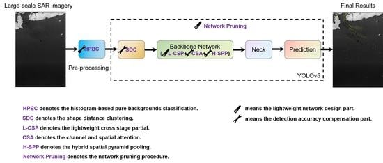
YOLOv5 is designed for optical images detection, which is not fully applicable to the field of on-board SAR ship detection. For on-board ship detection in large-scene Sentinel-1 SAR images, Lite-YOLOv5 is proposed. As shown in Figure 2, based on YOLOv5, Lite-YOLOv5 specifically injects (1) an LCB module to lighten the network without sacrificing much accuracy; (2) network pruning to obtain a much more compact network; (3) a HPBC module to effectively exclude pure background samples and suppress false alarms; (4) a SDC module to generate superior priori anchors; (5) a CSA module to enhance the SAR ships semantic feature extraction ability; and (6) a H-SPP model to increase the context information of the receptive field. Note that we use the raw SAR gray images as the input features. Following the paradigm of optical image object detection, we simply copy the single-channel SAR image to generate the three-channel SAR image. Therefore, in Figure 2, our SAR image input size is 800 × 800 × 3.
For the lightweight network design, we first inject the L-CSP module into the backbone network. It is used to lighten the network with a slight accuracy sacrifice, which will be introduced in detail in Section 2.3.1. Then, for a more compact network structure, network pruning is adopted among the backbone, neck, and prediction parts. The details will be introduced in Section 2.3.2.
For better feature extraction, we first preprocess the input Sentinel-1 SAR images by the proposed HPBC module to effectively exclude pure background samples. The details will be introduced in Section 2.4.1. It should be noted that the prior anchors of the existing algorithms are generated based on optical images object distribution, which is not applicable to SAR images with characteristics of small ship size and large ship aspect ratio. We use the SDC module to generate superior priori anchors, which will be described in detail in Section 2.4.2. In the backbone, the proposed CSA module and H-SPP module are embedded. The former is used to enhance the SAR ships semantic feature extraction ability, which will be introduced in detail in Section 2.4.3. The latter is used to increase the context information of the receptive field, which will be introduced in detail in Section 2.4.4.
Next, we will introduce the L-CSP module, network pruning, HPBC module, SDC module, CSA module, and H-SPP module in detail in the following subsections.
2.3. Lightweight Network Design
2.3.1. L-CSP Module
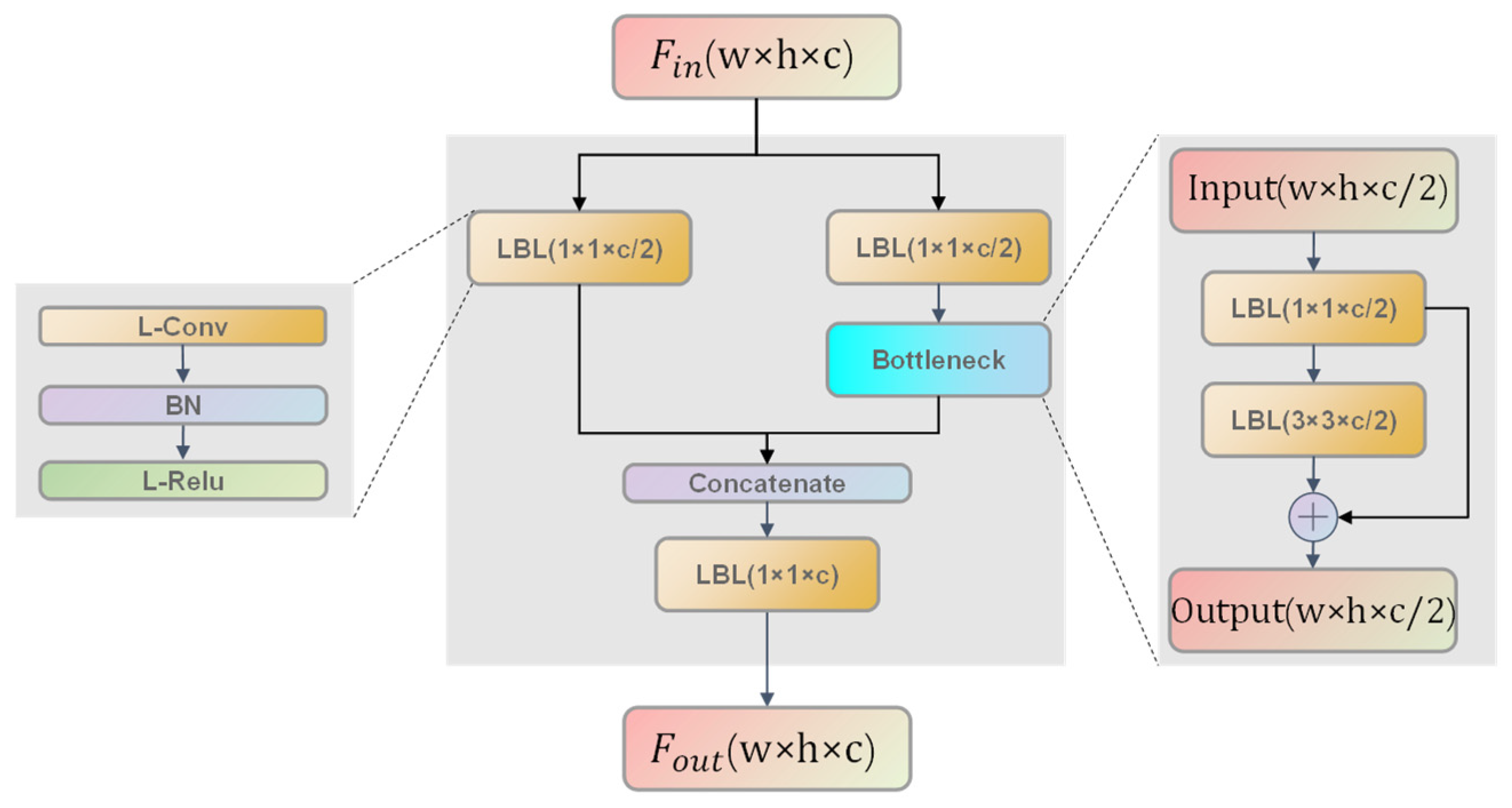
The lightweight cross stage partial (L-CSP) module mainly consists of a bottleneck structure and three convolutions. To obtain a lightweight backbone, L-CSP module adopts LBL units (i.e., a lightweight convolution layer (L-Conv), a BN layer, and an L-Relu activation layer) instead of the original CBL units (i.e., a Conv layer, a BN layer, and an L-ReLu activation layer).
Figure 3 shows the detailed structures of an L-CSP module. When the feature map Fin inputs, its transmission path is divided into two parallel branches as shown in Figure 3, where the channel of Fin is reduced by half to generate two new feature maps. Then, two feature maps of parallel branches are concatenated as a whole feature map (i.e., output feature map Fout).
Figure 4 shows the detailed structures of Conv and L-Conv, respectively. Figure 4a shows the architecture of the raw Conv. In practice, the input X ∈ RW × H × C, where W, H, and C represent the height, width, and channel of the input feature map, respectively. The convolution calculation formula is defined by
where ∗ is the convolution operation; f ∈ RC × K × K × H are the convolution filters, where K × K × N denotes the kernel size and channel of the convolution filters; and b denotes the bias of the convolution filters.
Figure 4b shows the architecture of the L-Conv. As we can see, only part of the input channels is utilized to generate intermediate feature maps, and the output feature maps are calculated from the obtained intermediate feature maps with low-cost linear operations (i.e., 3 × 3 convolution kernels). In this way, SAR ship features extraction becomes more efficient due to fewer floating-point operations.
Specifically, given the input X ∈ RW × H × C, M intermediate feature maps Y′ ∈ RW × H × C are obtained by using a convolution operation, i.e.,
where f′ ∈ RC × K × K × H are the convolution filters and M < N means there are fewer convolution filters than the original convolution block. To further obtain the N output feature maps, a series of low-cost linear operations are utilized to obtain the rest of feature maps. The calculation formula is defined by
where yi′ is the i-th intermediate feature maps of Y′ and Φi,j is the j-th (j < s) linear operation to calculate the j-th final output feature maps yi,j from the i-th intermediate feature maps of Y′. The last Φi,s is an identity mapping operation as shown in Figure 4b. Since there are m intermediate feature maps and s linear operations, we can obtain n = m × s final output feature maps, where the number of output feature maps is equal to the original convolution operations.
Since the computational complexity of linear operations is much less than that of ordinary convolution operations, L-Conv is a more lightweight convolution layer than Conv. Finally, by injecting the L-CSP module including L-Conv into the backbone, we can obtain a lightweight network architecture of low computational cost.
2.3.2. Network Pruning
The key of on-board ship detection is to find a lightweight on-board SAR ship detector that balances detection accuracy and model complexity under the constraints of satellites with limited memory and computation resources. Thus, it is of great significance to find a model compression method without much accuracy sacrifice. Network pruning is a mainstream model compression method. By pruning unimportant neurons, filters, or channels, it can effectively compress the parameters and computation of the model. Therefore, to further obtain a more compact detector, we follow the scheme illustrated in Figure 5 to prune the Conv and BN layers of the network.
From Figure 5, firstly, through sparse regularization training of the model, some parameters of the initial network tend to zero or equal to zero during training, and the neural network model with sparse weights is obtained. Then, the model is pruned to remove sparse channels. Next, the model is fine-tuned to restore the accuracy of the model. Finally, by iterating the above network pruning procedures, we can obtain the ultimate compact network.
The scaling factors, the sparsity training, the channel pruning, and fine-tuning will be illustrated below.
(1) Scale factors in BN layers: The Conv layer and BN layer are widely used in CNNs. In the Conv layer, reducing the number of filters can effectively reduce the amount of network parameters and computation, and accelerate the reasoning speed of the model. In the BN layer, the characteristic scaling coefficient of each BN layer corresponds to each channel, representing the activation degree of its corresponding channel. The operation formula of BN layer is formulated by
where Zin denotes input, Zout denotes output, μc and σc denote the mean and variance of input activation values, respectively, and α and β denote the scaling factor and offset factor corresponding to the activation channel, respectively.
In practice, the BN layers in our network are all followed after the Conv layers. Therefore, to prune a BN layer, it is necessary to prune the convolution kernel corresponding to the upper layer and subtract the channels of the convolution kernel corresponding to the next layer.
(2) Training with the L1 sparsity constraint: The sparse effect of L1 regularization on CNNs has been proved and widely used [38,39]. In this paper, a penalty factor is added to the loss function to constrain the weight of the Conv layer and the scaling coefficient of the BN layer, and the model will be sparse. The larger the regularization coefficient is, the greater the constraint is. Specifically, the sparsity constraint loss function is defined by
where Lossraw denotes the loss function of the raw detector, g(γ) = |γ| denotes L1 regularization, and λ denotes the regularization coefficient, adjusted according to the dataset.
During the sparsity training procedure of network pruning, we visualize the scale factors of BN layers. In general, the smaller the scale factor is, the sparser the channel parameters of the network are. We visualize the scale factors with three typical regularization factors (i.e., λ = 0, λ = 10−4, λ = 10−3), respectively, following [39]. Obviously, λ = 0 means there is no sparsity training (i.e., normal training). From Figure 6, when λ = 0, the scale factors distribution of the BN layer obeys an approximately normal distribution. When λ = 10−4, some scale factors are pressed towards 0, but not enough to guarantee the sparsity of scale factors. When λ = 10−3, most of the scale factors are pressed towards 0, which is enough to guarantee channel-wise pruning is being followed. Therefore, in our implementation, Lite-YOLOv5 is sparsity trained with λ = 10−3 to guarantee the channel-wise sparsity.
(3) Channel pruning and fine-tuning: After sparse regularization training, the model with more sparse weights is obtained and many weights are close to zero. Then, we prune the channels of the near-zero scaling factor by deleting all incoming and outcoming connections and corresponding weights. We prune the channels across all BN layers according to the prune ratio Pr, which is defined as a certain percentile of all the scaling factor values. This ratio Pr will be determined experimentally in Section 5.2.2. Then, we adopt fine-tuning for the pruned model to restore the accuracy. Note that fine-tuning is a simple training the same as normal training. However, in this way, we can obtain a lightweight detector without sacrificing too much accuracy. In addition, an iterative network pruning procedure can lead to a more compact network [28] as can be seen in Figure 5.
2.4. Detection Accuracy Compensation
2.4.1. HPBC Module
In an on-board SAR ship detection mission, quantities of pure backgrounds images will bring additional detection burden to the detector (pure background images mean that there are no ships in images). [24]. Based on the common sense that the ocean area is much larger than the land area, most of the pure background images are pure background ocean images. On the one hand, false alarms may occur even encountering pure background images, as seen in Figure 7; on the other hand, pure background images may only increase the detection time of the detector without any benefit.
From Figure 7, there are some false alarm examples of the DL detector. A DL detector without prior knowledge can be fooled when encountering ghost shadows, radio frequency interference, etc. In fact, many statistical models have been developed to describe SAR image data in the constant false alarm rate (CFAR)-based algorithms [40]. The analysis of a large number of measured data shows that Gamma distribution can be well applied to sea clutter modeling [41,42,43].
Thus, it is necessary to integrate the traditional mature methods with rich expert experience into the preprocessing of a DL detector, otherwise on-board SAR ship detection will be time-consuming and labor intensive.
For the first time, we bring traditional sea clutter modeling method into the preprocessing of a DL detector. Inspired by the sea clutter modeling method, we propose a simple but effective histogram-based pre-classification to process the SAR images. For brevity, it is noted as the histogram-based pure backgrounds classification (HPBC) module.
For a SAR image I, its histogram is to count the frequency of all pixels in I according to the size of the gray value, which reflects the statistical characteristics of I. The histogram can be described by
where ni denotes the occurrence numbers of pixels with the gray value i and n denotes the total numbers of pixels.
Note that the sea clutter sample is the ocean images. Moreover, sea clutter samples can be simply divided into pure background images and ships involved images. Figure 8a shows a typical pure background ocean image of sea clutter. Figure 8b shows its histogram and corresponding Gamma distribution curve. Figure 8c shows a typical ship image of sea clutter. Figure 8d shows its histogram and corresponding Gamma distribution curve. From Figure 8, one can conclude that sea clutter meets Gamma distribution.
On the one hand, a typical pure background ocean image means that the maximum of abscissa of its corresponding Gamma distribution curve is much less than 255 (i.e., A pure background sample means there is no strong scattering point, where the maximum pixels value of its histogram is much less than 255). On the other hand, a typical ship image means that the maximum of the abscissa of its corresponding Gamma distribution curve can be up to 255 (i.e., A ship target usually means a strong scattering point, where the maximum pixels value of its histogram can be up to 255).
The flow of the HPBC module is as follows.
Step 1: We simply divide the original large-scale images into 800 × 800 sub-images without overlap, which is kept the same as in Zhang et al. [24].
Step 2: We calculate the sub-images’ histograms one by one. Once the histogram of an image is the Gamma distribution and the maximal abscissa of its corresponding Gamma distribution curve is less than the threshold εa, we simply judge it as a pure back ground sample. This threshold εa will be determined experimentally in Section 5.3.
Step 3: A pure background ocean image will not be input to the detector. As a consequence, the HPBC module can suppress the number of false alarms (i.e., there may be some false alarms in pure background ocean images as seen in Figure 7). In addition, it is helpful to reduce the detection time of the detector. The above conclusions will be confirmed in Section 5.3.
Note that when the threshold εa is set higher, more images will be excluded. However, since we focus on not excluding the ship images by mistake, the threshold being equal to εa is fine (i.e., HPBC is only a rough preprocessing, and we would rather recognize fewer pure backgrounds than recognize the positive sample images as pure backgrounds).
2.4.2. SDC Module
The main idea of SDC is using the SAR ship shape distance to generate the superior prior anchors to match ship shape better. SDC is composed of the following steps.
First, k ground-truth anchors are randomly chosen as the k initialization prior anchors. Subsequently, for each ground-truth anchor, the cluster labels of the sample are calculated, which can be described by
where Li denotes the length of the i-th ground-truth anchor, Lj denotes the length of the j-th prior anchor, Wi denotes the width of the i-th ground-truth anchor, Wj denotes the width of the j-th prior anchor, ARi denotes the aspect ratio of the i-th ground-truth anchor, ARj denotes the aspect ratio of the j-th prior anchor, and labeli denotes the label of the i-th ground-truth anchor.
Then, the length, width, and aspect ratio of the j-th prior anchor are updated by the following formulas:
where nj denotes the number of ground-truth anchors belonging to the j-th prior anchors and Cj denotes the j-th cluster space.
Finally, iterate Formulas (7)–(10) until the following Formula (11) reaches the local optimal solution:
The K-means clustering algorithm is widely used in clustering problems owing to its simplicity and efficiency [44]. Therefore, in our paper, the prior anchors obtained by K-means and the SDC module are shown in Table 2. Figure 9a shows the cluster analysis of LS-SSDD-v1.0 by K-means. Figure 9b shows the cluster analysis of LS-SSDD-v1.0 by the SDC module.
From Figure 9, one can conclude that the proposed SDC module possesses a superior clustering performance (i.e., ~3.90 mean distance < ~4.96 mean distance compared with K-means). Subjectively, in Figure 9, the prior anchors clustered by the SDC module are smaller and roughly symmetrically distributed by the central axis, which conforms to the distribution law of LS-SSDD-v1.0 (i.e., there are numerous of small ships and the aspect ratio of ships is symmetrically distributed.). The above fully confirms the effectiveness of the SDC module.
2.4.3. CSA Module
The essence of the attention mechanism is to extract more valuable information for task objectives in the target area and to suppress or ignore some irrelevant details. Channel attention focuses on the “what” problem, (i.e., it focuses on what plays an important role in the whole image). However, in general, a ship in the image is sparsely distributed and its pixel proportion is quite small. Thus, only part of the pixel space in a ship detection task is valuable. Spatial attention focuses on the “where” problem, (i.e., where the ship is in the whole image). Spatial attention is the supplement of channel attention; each spatial feature is selectively aggregated through the weighting of spatial features. Therefore, different from SENet [45], which only focuses on channel attention, we bring channel and spatial attention simultaneously, named as the CSA Module.
To achieve this, we sequentially apply channel and spatial attention. From Figure 10, given the input feature map F ∈ RW × H × C, channel attention can generate channel weight WC ∈ RC × 1 × 1 and spatial attention can generate spatial weight WS ∈ RH × W × 1. The different depths of color in Figure 10 represent different values of weights.
Specifically, for channel attention, given the input feature map F ∈ RW × H × C, first, global average pooling (GAP) [46] is carried out to generate the average spatial response and global max pooling (GMP) [46] to generate the maximum spatial response; then, they are transmitted, respectively, to the multi-layer perceptron (MLP) to encode the channel information, which is helpful to infer finer channel attention; next, element-wise addition is conducted between the two feature maps; then, the synthetic channel information is activated through the sigmoid function to obtain the channel weight feature map, i.e., a channel weight matrix WC; finally, element-wise multiplication is conducted between the original feature map F ∈ RW × H × C and obtained channel weight matrix WC.
In short, the above can be defined by
where F′ denotes the weighted feature map, F denotes the input feature map, ⊙ denotes element-wise multiplication, and WC denotes the obtained channel weight matrix, i.e.,
where GAP denotes the global average-pooling operation, GMP denotes the global max-pooling operation, ⊕ denotes element-wise summation, fc-encode denotes the channel coder, and σ denotes the sigmod activation function.
As for spatial attention, given the input feature map F′ ∈ RC × W × H, first, global average pooling (GAP) [46] is carried out to generate the average spatial response and global max pooling (GAP) [46] is carried it to generate the maximum spatial response; then, the two generated results are concatenated as a whole feature map; next, a space encoder of our design is used to encode the space information, which is helpful to infer finer spatial attention; then, it is activated through the sigmoid function to obtain the spatial weight feature map, i.e., a spatial weight matrix WS; finally, element-wise multiplication is conducted between the original feature map F′ ∈ RC × W × H and the obtained spatial weight matrix WS.
In short, the above can be defined by
where F″ denotes the weighted feature map, F′ denotes the input feature map, ⨀ denotes element-wise multiplication, and WS denotes the obtained spatial weight matrix, i.e.,
where GAP denotes the global average-pooling operation, GMP denotes the global max-pooling operation, © denotes concatenation operation, fs-encode denotes the space coder, and σ denotes the sigmod activation function.
Finally, we can obtain a finer channel and space information. With the CAS module inserted into the network, each level can extract both rich spatial and rich semantic information, which is helpful to improve the detection performance of small ships.
2.4.4. H-SPP Module
In the CV community, by capturing rich context information, the network can better understand the relationship between pixels and enhance the performance of detection. For aggregating context information, a pyramid pooling module with max-pooling has been commonly adopted so far [47,48,49]. The previous works believe that since the object of interest may produce the largest pixel value, adopting max-pooling is enough. We argue that average-pooling gathers another important clue about global information extraction capacity. This idea is inspired by the works of [29], which is recommended for readers. Thus, we adopt a hybrid spatial pyramid pooling (H-SPP) module to further enhance the global context information extraction capacity of the network. It can be aware of both local and global contents of feature maps, and attach importance to key small ship features.
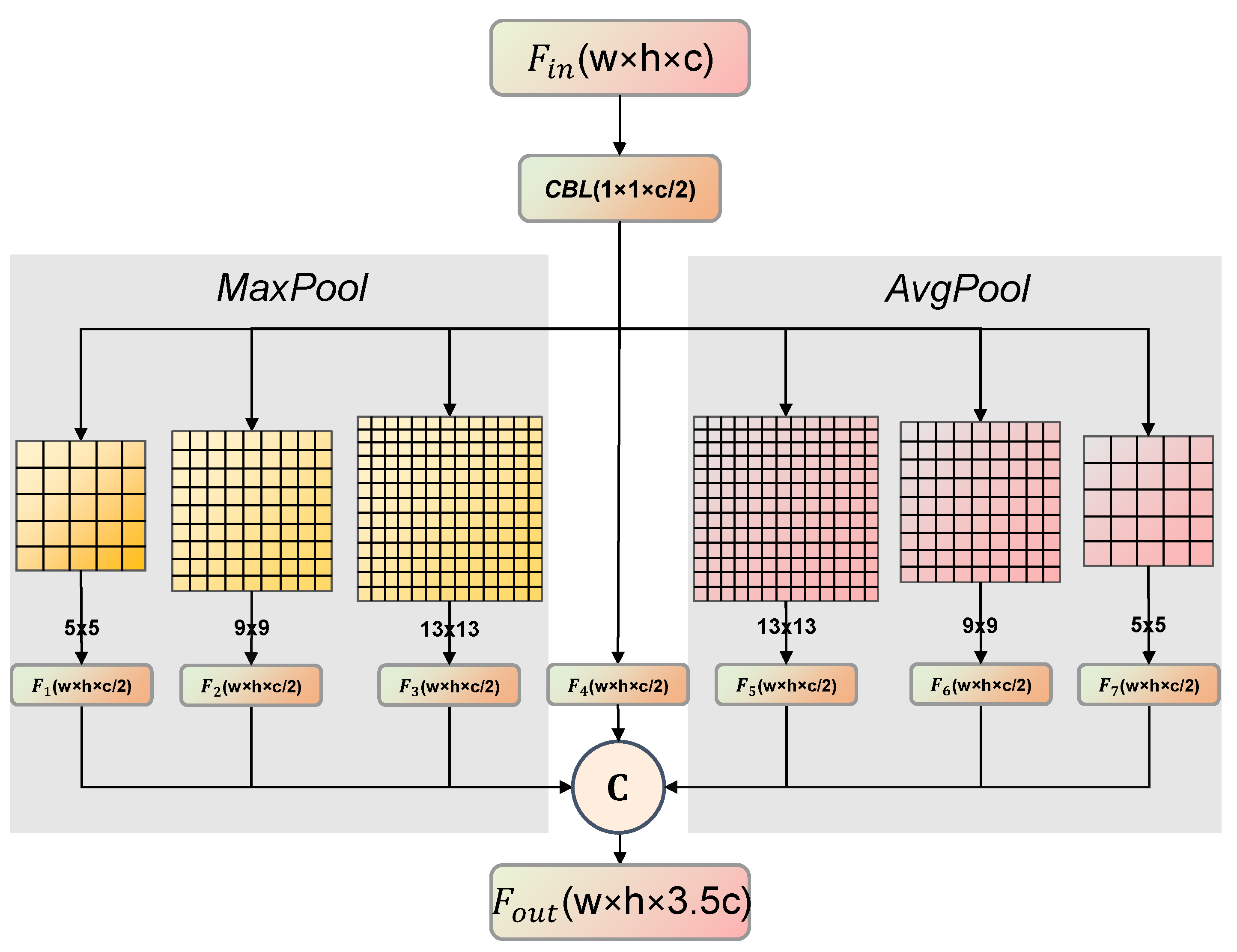
Different from previous works [47,48,49], the H-SPP module mainly aggregates the feature map generated by both average-pooling and max-pooling operations with different pooling sizes. Figure 11 shows the detailed structures of the H-SPP module. Then, we will further introduce the principle of the H-SPP module.
The H-SPP module aggregates the feature map generated by both the max-pooling layer and average-pooling layer of different kernel sizes (i.e., 5 × 5, 9 × 9 and 13 × 13), as shown in Figure 11. Specifically, given the input feature map Fin ∈ RW × H × C generated by the backbone, it is first transmitted to a CBL module to generate a feature map F′ ∈ RW × H × 0.5C with refined channel information. Then, (1) max-pooling of different kernel sizes (i.e., 5 × 5, 9 × 9 and 13 × 13) is simultaneously carried out to generate three local receptive field feature maps and (2) average-pooling of different kernel sizes (i.e., 5 × 5, 9 × 9 and 13 × 13) is carried out to generate three global receptive field feature maps. Next, six generated results and original ones (i.e., F1–F7 from Figure 11) are concatenated as a synthetic feature map. Finally, the feature map level fusion of local features and global features is realized, which enriches the expression ability of the final feature map Fout ∈ RW × H × 3.5C.
In short, the above can be defined by
where Conv1 × 1 denotes the 1 × 1 convolution operation, MaxPool denotes the max-pooling operations (with kernel sizes of 5 × 5, 9 × 9 and 13 × 13, respectively), AvgPool denotes the average-pooling operations (with kernel sizes of 5 × 5, 9 × 9, and 13 × 13, respectively), and © denotes the concatenation operation.
By aggregating the feature maps of abundant receptive fields, the H-SPP module obtains different degrees of context information, and enhances the network’s ability to capture both local and global information. Thus, the H-SPP module can improve the accuracy of the final prediction result of the algorithm. In this paper, the H-SPP module will be used to further improve the detection performance of Lite-YOLOv5.
3. Experiments
Different from the traditional integrated training and testing platform, we first used a workstation with the powerful NVIDIA RTX3090 as the training experiment platform to generate the well-trained detector Lite-YOLOv5, then we used a NVIDIA Jetson TX2 as the training experiment platform to evaluate the on-board SAR ship detection ability of Lite-YOLOv5.
3.1. Experimental Platform
3.1.1. Training Experimental Platform
Considering the limited computing resources and computing power of NVIDIA Jetson TX2, we used the workstation with the GPU model of NVIDIA RTX3090, CPU model of i7-10700, and memory size of 32 G to carry out the training part of the experiment. PyTorch 1.7.0 [50] based on the Python 3.8 language was adopted as the framework of our algorithm. We also used CUDA11.1 in our experiments to call the GPU for training acceleration. Subsequently, we transplanted the trained model into the NVIDIA Jetson TX2.
3.1.2. Testing Experimental Platform
We used the NVIDIA Jetson TX2 as the development board in order to realize on-board ship detection during the testing part of experiment. The NVIDIA Jetson TX2 is an embedded vision computer system with the 256-core NVIDIA Maxwell GPU model, dual-core Denver2 CPU model, and an 8 G memory size. Meanwhile, the characteristics of low power consumption, high performance, large memory bandwidth, etc. make it very suitable for on-board satellite data processing.
3.2. Dataset
The LS-SSDD-v1.0 dataset is widely used for SAR image intelligent interpretation [51,52,53,54]. The characteristic of small ships with large-scale backgrounds in LS-SSDD is close to actual satellite images; thus, we adopted the LS-SSDD-v1.0 dataset to verify the effectiveness of Lite-YOLOv5. Table 3 shows the details of the LS-SSDD dataset.
From Table 3, there are 15 large-scale images (cover width ~250 km) numbered by 00.jpg to 15.jpg from different places (Tokyo, Adriatic Sea, etc.), polarizations (VV, VH), and scenes (land, sea). Considering the computing power of the GPU, we simply divided the original large-scale images into 800 × 800 sub-images without embellishment, keeping to the method of Zhang et al. [24]. Since there were fifteen 24,000 pixels × 16,000 pixels large-scale images, the total sub-image number was 9000. Finally, according to Zhang et al. [24], the LS-SSDD-v1.0 dataset was divided into a training set for training learning and a test set for result performance evaluation via the ratio of 2:1.
3.3. Experimental Details
We employed the stochastic gradient descent (SGD) [55] algorithm to train our network. The network input size was 800 pixels × 800 pixels and the batch size of 16 was adopted. During normal and sparsity training, we trained the network for 100 total epochs. We also set the learning rate as 0.001, the weight decay as 0.0005, and the momentum as 0.937. Other hyper-parameters not mentioned were kept the same as those in YOLOv5.
3.4. Evaluation Indices
Precision (P) is calculated by
where # denotes the number, TP denotes the situation where the prediction and label are both ships, and FP denotes the situation where the prediction is a ship but the label is the background.
Recall (R) is calculated by
where FN denotes the situation where the prediction is the background but the label is a ship.
The average precision (AP) is calculated by
where P denotes the precision, and R denotes the recall.
F1 can take account of both precision and recall and is calculated by
Finally, t denotes the inference consuming time of a sub-image detection. As a result, the running time T of a large-scale image is equal to 600 t. Moreover, in order to evaluate the portability performance of Lite-YOLOv5 on on-board SAR ship detection, we also calculated the parameter size, FLOPs, and model volume.
4. Results
4.1. Quantitative Results
Table 4 shows the quantitative results of Lite-YOLOv5 on the LS-SSDD-v1.0 dataset. In Table 4, we can see the detection performance comparison with the raw YOLOv5. The ablation studies about the influence of each proposed module will be introduced in detail in Section 5 by the means of each installation and removal.
From Table 4, one can conclude that:
- Compared with YOLOv5, our Lite-YOLOv5 can guarantee the model is lightweight and realize the slight improvement of detection performance at the same time.
- On the one hand, as for accuracy indices, Lite-YOLOv5 can make a 5.97% precision improvement (i.e., from 77.04% to 83.01%), 1.12% AP improvement (i.e., from 72.03% to 73.15%), and 1.51% F1 improvement (i.e., from 72.01% to 73.52%). This fully reveals the effectiveness of the proposed HPCB, SDC, CSA, and H-SPP modules.
- On the other hand, as for other evaluation indices, Lite-YOLOv5 can realize on-board ship detection with 37.51 s per large-scale image (73.29% of the processing time of YOLOv5), a lighter architecture with 4.44 G FLOPs (26.59% of the FLOPs of YOLOv5), and 2.38 M model volume (14.18% of the model size of YOLOv5). This fully reveals the effectiveness of the proposed L-CSP module and network pruning.
Table 5 shows the performance comparisons of Lite-YOLOv5 with eight other state-of-the-art detectors. In Table 5, we mainly select the Libra R-CNN [56], Faster R-CNN [57], EfficientDet [58], free anchor [59], FoveaBox [60], RetinaNet [61], SSD-512 [62], and YOLOv5 [27] for comparison. They were all trained on the LS-SSDD-v1.0 dataset with loading ImageNet pre-training weights. Their implementations were also kept basically the same as in the original report. In addition, it should be emphasized that there is no end-to-end on-board SAR ship detector. Thus, we selected the mainstream two-stage detector (i.e., Libra R-CNN, Faster R-CNN) and single-stage detectors (i.e., EfficientDet, free anchor, FoveaBox, RetinaNet, SSD-512, and YOLOv5) in the CV community for comparison.
From Table 5, the following conclusions can be drawn:
- What stands out in this table is the competitive accuracy performance with the greatly reduced model volume of Lite-YOLOv5.
- The AP and F1 of Lite-YOLOv5 cannot reach the best performance at the same time; nevertheless, the excellent performance of the other evaluation indicators can make up for it. More prominently, with the tiny model size of ~2 M and competitive accuracy indicators, Lite-YOLOv5 can ensure a superior on-board detection performance.
- Compared with the experimental baseline YOLOv5, Lite-YOLOv5 offers ~1.1% AP improvement (i.e., from 72.03% to 73.15%) and ~1.5% F1 improvement (i.e., from 72.01% to 73.52%). This fully reveals the effectiveness of the proposed HPBC, SDC, CSA, and H-SPP modules.
- Compared with the experimental baseline YOLOv5, Lite-YOLOv5 offers the most lightweight network architecture with 4.44 G FLOPs (~26.6% of the FLOPs of YOLOv5), 1.04 M parameter size (~14.7% of the parameter size of YOLOv5), and ~ 2 M model volume (~14.2% of the model size of YOLOv5). This fully reveals the effectiveness of the proposed L-CSP module and network pruning.
- Libra R-CNN offers the highest F1 (i.e., 75.93%), but its AP is rather poor to satisfy the basic detection application, i.e., its 62.90% AP << Lite-YOLOv5′s 73.15%. Furthermore, its detection time, FLOPs, parameter size, and model volume are all one or two orders of magnitude than those of Lite-YOLOv5, which is a huge obstacle for on-board detection.
4.2. Qualitative Results
Figure 12 shows the visualization results on the LS-SSDD-v1.0 as an example. As we can see, Lite-YOLOv5 can carry out accurate SAR ship detection even in difficult conditions (i.e., larger scene image, multi-scale ships, and different aspect ratios of ships).
Figure 13 shows the detection results of different methods under complicated scenarios (i.e., offshore scenes of strong speckle noise and inshore scenes). Note that we only chose some lightweight models for fair comparison.
From Figure 13, one can conclude the following:
- In the offshore scenes, Lite-YOLOv5 can offer high-quality detection results even under the environment of strong speckle noise. Most other methods always produce the missed alarms caused by speckle noise. Taking the second line of images as an example, there were four missed detections of RetinaNet and three missed detections of YOLOv5, which are both more than that of Lite-YOLOv5 (only one missed ship).
- In the inshore scenes, Lite-YOLOv5 can offer high-quality detection results even under the environment of ship-shaped reefs and buildings near shore. Most other methods always produce the missed alarms caused by them. Taking the fourth line of images as an example, there were two missed detections of RetinaNet and two missed detections of YOLOv5, which are both more than that of Lite-YOLOv5 (only one missed ship).
- Lite-YOLOv5 can offer an advanced on-board ship detection performance compared with other state-of-the-art methods.
5. Ablation Study
In this section, we will introduce the ablation studies to show the influence of each proposed module by the means of each installation and removal.
5.1. Ablation Study on the L-CSP Module
Table 6 shows the ablation study of Lite-YOLOv5 with and without the L-CSP module. In Table 6, “✘” means Lite-YOLOv5 without the L-CSP module (while keeping the other five modules), while “✓” means Lite-YOLOv5 with the L-CSP module (i.e., our proposed detector). From Table 6, one can find that the L-CSP module can guarantee a lighter architecture with 4.44 G FLOPs and a 2.38 M model volume (~45.6% decrease of FLOPs and ~7.0% decline of model volume when compared with Lite-YOLOv5 without the L-CSP module), which confirms that the L-CSP module can offers a model with greatly reduced computation. In addition, there is only a slight decrease to the overall detection performance. Thus, the L-CSP module can realize a model of sharply reduced computation with only a slight accuracy loss, which confirms its superior cost-effectiveness in lightweight network design.
5.2. Ablation Study on Network Pruning
We conducted two ablation experiments on network pruning. Experiment 1 in Section 5.2.1 shows the effectiveness of network pruning in Lite-YOLOv5. Experiment 2 in Section 5.2.2 shows the effectiveness of channel-wise pruning in network pruning.
5.2.1. Experiment 1: Effectiveness of Network Pruning
Table 7 shows the ablation study of Lite-YOLOv5 with and without network pruning. In Table 7, “✘” means Lite-YOLOv5 without network pruning (while keeping the other five modules), while “✓” means Lite-YOLOv5 with network pruning (i.e., our proposed detector). From Table 7, one can find that network pruning can realize a lighter architecture with 4.44 G FLOPs and a 2.38 M model volume (~68.6% decrease of FLOPs and ~81.5% decline of model volume when compared with Lite-YOLOv5 without network pruning). Thus, network pruning can achieve a huge compression of the model with a slight accuracy loss, which confirms its superior performance in lightweight network design. In addition, we also conducted another experiment to explore the effect of channel-wise pruning.
5.2.2. Experiment 2: Effect of Channel-Wise Pruning
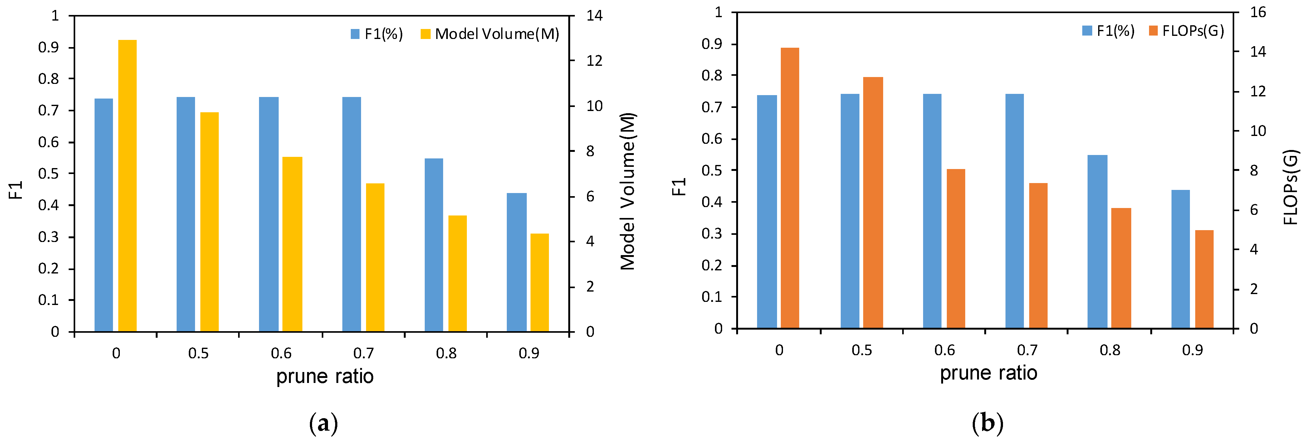
During the channel pruning procedure of network pruning, we conducted several experiments under different pruning ratios Pr. In general, the larger the pruning ratio is, the smaller the model volume of the network is while the poorer the model performance is. Thus, it is of great importance to trade off the pruning ratio and the model performance. From Figure 14, we can see the effect of choosing different pruning ratios from Lite-YOLOv5 trained on LS-SSDD-v1.0 with λ = 10−3. When Pr goes beyond 0.7, the F1 of the model seriously deteriorates. Thus, in our implementation, Lite-YOLOv5 is channel-wise pruned with a Pr equal to 0.7 to trade off the model performance and model complexity.
5.3. Ablation Study on the HPBC Module
Table 8 shows the ablation study of Lite-YOLOv5 with and without the HPBC module. In Table 8, “✘” means Lite-YOLOv5 without the HPBC module (while keeping the other five modules), while “✓” means Lite-YOLOv5 with the HPBC module (i.e., our proposed detector). From Table 8, one can find that the HBC module can make a ~0.2% improvement with AP and F1. Note that the ~0.7% improvement in precision (i.e., the decrease of false alarms) reveals the reason of the improvement of overall detection performance (i.e., the HPBC module can effectively exclude pure background ocean images, so some false alarms in them are avoided). Furthermore, the HBC module can obtain the real-time detection performance with only a 37.51 s running time for one large-scale image (~10.4 s decrease of running time compared with Lite-YOLOv5 without the HPBC module).
All of the above reveal that the HPBC module can effectively classify pure background ocean images; thus, it can (1) suppress some false alarms, and therefore the overall accuracy indices are increased and (2) decrease the detection burden of the detector, and therefore real-time detection performance is guaranteed. Significantly, one may find more powerful techniques to further classify the pure background samples, but HPBC might be one of the most direct approaches without complicated steps and obscure theories.
We performed another experiment to study the impact of the abscissa filter threshold εa. The experimental results are shown in Table 9. It can be concluded that when εa is set higher, more pure background ocean images will be excluded (i.e., fewer images remain) and detection performance will be improved. However, in the actual scene, we focus on not excluding the ship images by mistake. Thus, it is of great importance to optimize εa on the basis of guaranteeing the original number of ship images. In Table 9, εa being set to 128 is the optimal choice for the balance of the number of ship images and detection accuracy. Thus, the final εa is set to 128 in Lite-YOLOv5.
5.4. Ablation Study on the SDC Module
Table 10 shows the ablation study of Lite-YOLOv5 with and without the SDC module. In Table 10, “✘” means Lite-YOLOv5 without the SDC module (while keeping the other five modules), while “✓” means Lite-YOLOv5 with the SDC module (i.e., our proposed detector). From Table 10, one can find that the SDC module can make an overall detection performance improvement with a ~ 0.9% F1 improvement, which confirms its effectiveness. This is because the SDC module can utilize the SAR ship shape distance (i.e., the distribution of length, width, and aspect ratio) to generate a more appropriate prior anchor. Finally, Lite-YOLOv5 can extract SAR ship information more effectively. In addition, the SDC module brings hardly any model complexity increase, which confirms its superior cost-effectiveness in detection accuracy compensation.
5.5. Ablation Study on the CSA Module
Table 11 shows the ablation study of Lite-YOLOv5 with and without the CSA module. In Table 11, “✘” means Lite-YOLOv5 without the CSA module (while keeping the other five modules), while “✓” means Lite-YOLOv5 with the CSA module (i.e., our proposed detector). From Table 11, one can find that the CSA module can make an overall detection performance improvement with a ~2.6% AP and ~1.9% F1 improvement, which confirms its effectiveness. This is because the CSA module can extract both rich spatial and rich semantic information. Finally, Lite-YOLOv5 can improve the ship detection performance. In addition, the CSA module only brings a slight model complexity increase, which confirms its superior cost-effectiveness in detection accuracy compensation.
5.6. Ablation Study on the H-SPP Module
Table 12 shows the ablation study of Lite-YOLOv5 with and without the H-SPP module. In Table 12, “✘” means Lite-YOLOv5 without the H-SPP module (while keeping the other five modules), while “✓” means Lite-YOLOv5 with the H-SPP module (i.e., our proposed detector). From Table 12, one can find that the H-SPP module can make an overall detection performance improvement with a ~0.8% F1 improvement, which confirms its effectiveness. This is because the H-SPP module can aggregate the feature maps of abundant receptive fields and obtain different degrees of context information. Finally, Lite-YOLOv5 can effectively improve the network’s capacity to capture both local and global information of SAR images. In addition, the H-SPP module only brings a slight model complexity increase, which confirms its superior cost-effectiveness in detection accuracy compensation.
6. Discussion
The above experiments and ablation studies verify the effectiveness of Lite-YOLOv5. We can transplant it to the embedded platform NVIDIA Jetson TX2 on the SAR satellite for on-board SAR ship detection. The combination of six optimization characters (i.e., L-CSP, network pruning, HPBC, SDC, CSA, and H-SPP) guarantee the advanced on-board ship detection performance. As for the on-board processing, firstly, we cut the large-scale SAR imagery into 800 pixels × 800 pixels image patches without embellishment. Then, we conduct ship detection using Lite-YOLOv5. Finally, the obtained detection results on patches are coordinate mapped to obtain the final large-scale SAR ship results. In this way, only the ship sub-images and corresponding coordinates will be transmitted to the ground station, which is of great significance to utilize real-time and accurate ship information, especially in emergencies.
In addition, the all of the above show that Lite-YOLOv5 possesses an advanced on-board SAR ship detection performance. In order to obtain better and faster ship detection results, the follow-up work will need to explore the reasonable hardware acceleration strategy of the platform. Aiming at giving full play to the computing power of the NVIDIA Jetson TX2 hardware, we will allocate each module to the appropriate hardware to maximize the computing efficiency and obtain more efficient detection results. In addition, there are many other feasible schemes in lightweight model design (such as knowledge distillation). Therefore, our future work will explore distillation techniques.
7. Conclusions
This paper proposes a lightweight on-board SAR ship detector called Lite-YOLOv5, which (1) reduces the model volume; (2) decreases the floating-point operations (FLOPs), and (3) guarantees the on-board ship detection without sacrificing accuracy. First, two characteristics are used to obtain a lightweight network, i.e., (1) a LCB module is inserted into the backbone network of YOLOv5 and (2) network pruning is applied to obtain a more compact model. Then, four characteristics are used to guarantee the detection accuracy, i.e., (1) an HPCB module to effectively exclude pure background samples and suppress the false alarms; (2) a SDC method to generate superior priori anchor; (3) a CSA model to enhance the SAR ships semantic feature extraction ability; an (4) an H-SPP model to increase the context information of the receptive field. To evaluate the on-board SAR ship detection ability of Lite-YOLOv5, we also transplanted it to the embedded platform NVIDIA Jetson TX2. Experimental results on the Large-Scale SAR Ship Detection Dataset-v1.0 (LS-SSDD-v1.0) show that Lite-YOLOv5 can realize a lighter architecture with a 2.38 M model volume (14.18% of the model size of YOLOv5), on-board ship detection with a low computation cost (26.59% of FLOPs of YOLOv5), and superior detection accuracy (1.51% F1 improvement compared with YOLOv5). We also conducted a large quantity of ablation experiments to verify the effectiveness of the proposed modules. Thus, Lite-YOLOv5 can provide high-performance on-board SAR ship detection, which is of great significance.
In the future, our works will be as follows:
- We will decrease the detection time further.
- We will lighten the detector further without sacrificing the accuracy.
- We will explore a reasonable hardware acceleration scheme for on-board SAR ship detection.
- We will explore other viable approaches such as distillation techniques in the following lightweight detector design.
Author Contributions
Conceptualization, X.X.; methodology, X.X.; software, X.X.; validation, T.Z.; formal analysis, T.Z.; investigation, X.X.; resources, X.X.; data curation, X.X.; writing—original draft preparation, X.X.; writing—review and editing, T.Z.; visualization, T.Z.; supervision, T.Z.; project administration, T.Z.; funding acquisition, X.Z. All authors have read and agreed to the published version of the manuscript.
Funding
This research received no external funding.
Institutional Review Board Statement
Not applicable.
Informed Consent Statement
Not applicable.
Data Availability Statement
No new data were created or analyzed in this study. Data sharing is not applicable to this article. The LS-SSDD-v1.0 dataset provided by Tianwen Zhang is available from https://github.com/TianwenZhang0825/LS-SSDD-v1.0-OPEN (accessed on 6 February 2022) to download for scientific research.
Acknowledgments
The authors would like to thank the editors and anonymous reviewers for their valuable comments that greatly improved our manuscript.
Conflicts of Interest
The authors declare no conflict of interest.
Appendix A
For the reader’s convenience, in Table A1 we list all of the abbreviations and corresponding full name involved in this paper. The abbreviations are arranged in alphabetical order.

Table A1.
The abbreviations and corresponding full names.
| Abbreviation | Full Name |
|---|---|
| AP | average precision |
| BN | batch normalization |
| Conv | convolution |
| CFAR | constant false alarm rate |
| CNN | convolutional neural network |
| CSA | channel and spatial attention |
| CSP | cross stage partial |
| CV | computer vision |
| DAPN | dense attention pyramid network |
| DL | deep learning |
| DS-CNN | depth-wise separable convolution neural network |
| FFEN | fusion feature extraction network |
| FL | focal loss |
| FLOPs | floating point operations |
| FPN | feature pyramid network |
| GAP | global average pooling |
| GMP | global max pooling |
| HR-SDNet | high-resolution ship detection network |
| HNM | hard negative mining |
| HPBC | histogram-based pure backgrounds classification |
| H-SPP | hybrid spatial pyramid pooling |
| L-Conv | lightweight convolution |
| L-CSP | lightweight cross stage partial |
| LFO-Net | lightweight feature optimization network |
| L-Relu | Leaky_ReLu |
| LS-SSDD-v1.0 | Large-Scale SAR Ship Detection Dataset-v1.0 |
| MLP | multi-layer perceptron |
| NLP | natural language processing |
| PAN | path aggregation network |
| RDN | refined detection network |
| RPN | region proposal network |
| SAR | synthetic aperture radar |
| SDC | shape distance clustering |
| SGD | stochastic gradient descent |
| SPP | spatial pyramid pooling |
| YOLOv5 | You Only Look Once version 5 |
References
- Zhang, T.; Zhang, X.; Li, J.; Xu, X.; Wang, B.; Zhan, X.; Xu, Y.; Ke, X.; Zeng, T.; Su, H.; et al. SAR Ship Detection Dataset (SSDD): Official Release and Comprehensive Data Analysis. Remote Sens. 2021, 13, 3690. [Google Scholar] [CrossRef]
- Lin, Z.; Ji, K.; Leng, X.; Kuang, G. Squeeze and Excitation Rank Faster R-CNN for Ship Detection in SAR Images. IEEE Geosci. Remote Sens. Lett. 2019, 16, 751–755. [Google Scholar] [CrossRef]
- Xu, X.; Zhang, X.; Zhang, T. Multi-Scale SAR Ship Classification with Convolutional Neural Network. In Proceedings of the IEEE International Geoscience and Remote Sensing Symposium (IGARSS), Online Event, 11–16 July 2021; pp. 4284–4287. [Google Scholar]
- Zhang, T.; Zhang, X.; Ke, X. Quad-FPN: A Novel Quad Feature Pyramid Network for SAR Ship Detection. Remote Sens. 2021, 13, 2771. [Google Scholar] [CrossRef]
- O’Shea, T.; Hoydis, J. An Introduction to Deep Learning for the Physical Layer. IEEE Trans. Cogn. Commun. Netw. 2017, 3, 563–575. [Google Scholar] [CrossRef] [Green Version]
- Aceto, G.; Ciuonzo, D.; Montieri, A.; Pescapé, A. Mobile Encrypted Traffic Classification Using Deep Learning: Experimental Evaluation, Lessons Learned, and Challenges. IEEE Trans. Netw. Serv. Manag. 2019, 16, 445–458. [Google Scholar] [CrossRef]
- Liu, G.; Li, L.; Jiao, L.; Dong, Y.; Li, X. Stacked Fisher autoencoder for SAR change detection. Pattern Recognit. 2019, 96, 106971. [Google Scholar] [CrossRef]
- Ciuonzo, D.; Carotenuto, V.; De Maio, A. On Multiple Covariance Equality Testing with Application to SAR Change Detection. IEEE Trans. Signal Process. 2017, 65, 5078–5091. [Google Scholar] [CrossRef]
- Kang, M.; Ji, K.; Leng, X.; Lin, Z. Contextual Region-Based Convolutional Neural Network with Multilayer Fusion for SAR Ship Detection. Remote Sens. 2017, 9, 860. [Google Scholar] [CrossRef] [Green Version]
- Jiao, J.; Zhang, Y.; Sun, H.; Yang, X.; Gao, X.; Hong, W.; Fu, K.; Sun, X. A Densely Connected End-to-End Neural Network for Multiscale and Multiscene SAR Ship Detection. IEEE Access. 2018, 6, 20881–20892. [Google Scholar] [CrossRef]
- Cui, Z.; Li, Q.; Cao, Z.; Liu, N. Dense Attention Pyramid Networks for Multi-Scale Ship Detection in SAR Images. IEEE Trans. Geosci. Remote Sens. 2019, 57, 8983–8997. [Google Scholar] [CrossRef]
- Liu, N.; Cao, Z.; Cui, Z.; Pi, Y.; Dang, S. Multi-Scale Proposal Generation for Ship Detection in SAR Images. Remote Sens. 2019, 11, 526. [Google Scholar] [CrossRef] [Green Version]
- Wang, J.; Lu, C.; Jiang, W. Simultaneous Ship Detection and Orientation Estimation in SAR Images Based on Attention Module and Angle Regression. Sensors 2018, 18, 2851. [Google Scholar] [CrossRef] [Green Version]
- An, Q.; Pan, Z.; Liu, L.; You, H. DRBox-v2: An Improved Detector With Rotatable Boxes for Target Detection in SAR Images. IEEE Trans. Geosci. Remote Sens. 2019, 57, 8333–8349. [Google Scholar] [CrossRef]
- Chen, C.; Hu, C.; He, C.; Pei, H.; Pang, Z.; Zhao, T. SAR Ship Detection Under Complex Background Based on Attention Mechanism. In Image and Graphics Technologies and Applications; Springer: Singapore, 2019; pp. 565–578. [Google Scholar]
- Dai, W.; Mao, Y.; Yuan, R.; Liu, Y.; Pu, X.; Li, C. A Novel Detector Based on Convolution Neural Networks for Multiscale SAR Ship Detection in Complex Background. Sensors 2020, 20, 2547. [Google Scholar] [CrossRef] [PubMed]
- Wei, S.; Su, H.; Ming, J.; Wang, C.; Yan, M.; Kumar, D.; Shi, J.; Zhang, X. Precise and Robust Ship Detection for High-Resolution SAR Imagery Based on HR-SDNet. Remote Sens. 2020, 12, 167. [Google Scholar] [CrossRef] [Green Version]
- Chang, Y.-L.; Anagaw, A.; Chang, L.; Wang, Y.C.; Hsiao, C.-Y.; Lee, W.-H. Ship Detection Based on YOLOv2 for SAR Imagery. Remote Sens. 2019, 11, 786. [Google Scholar] [CrossRef] [Green Version]
- Zhang, T.; Zhang, X.; Shi, J.; Wei, S. Depthwise Separable Convolution Neural Network for High-Speed SAR Ship Detection. Remote Sens. 2019, 11, 2483. [Google Scholar] [CrossRef] [Green Version]
- Mao, Y.; Yang, Y.; Ma, Z.; Li, M.; Su, H.; Zhang, J. Efficient Low-Cost Ship Detection for SAR Imagery Based on Simplified U-Net. IEEE Access. 2020, 8, 69742–69753. [Google Scholar] [CrossRef]
- Zhang, X.; Wang, H.; Xu, C.; Lv, Y.; Fu, C.; Xiao, H.; He, Y. A Lightweight Feature Optimizing Network for Ship Detection in SAR Image. IEEE Access. 2019, 7, 141662–141678. [Google Scholar] [CrossRef]
- Wang, Y.; Wang, C.; Zhang, H.; Dong, Y.; Wei, S. Automatic Ship Detection Based on RetinaNet Using Multi-Resolution Gaofen-3 Imagery. Remote Sens. 2019, 11, 531. [Google Scholar] [CrossRef] [Green Version]
- Wang, Y.; Wang, C.; Zhang, H.; Dong, Y.; Wei, S. A SAR Dataset of Ship Detection for Deep Learning under Complex Backgrounds. Remote Sens. 2019, 11, 765. [Google Scholar] [CrossRef] [Green Version]
- Zhang, T.; Zhang, X.; Ke, X.; Zhan, X.; Shi, J.; Wei, S.; Pan, D.; Li, J.; Su, H.; Zhou, Y.; et al. LS-SSDD-v1.0: A Deep Learning Dataset Dedicated to Small Ship Detection from Large-Scale Sentinel-1 SAR Images. Remote Sens. 2020, 12, 2997. [Google Scholar] [CrossRef]
- Xu, P.; Li, Q.; Zhang, B.; Wu, F.; Zhao, K.; Du, X.; Yang, C.; Zhong, R. On-Board Real-Time Ship Detection in HISEA-1 SAR Images Based on CFAR and Lightweight Deep Learning. Remote Sens. 2021, 13, 1995. [Google Scholar] [CrossRef]
- Han, K.; Wang, Y.H.; Tian, Q.; Guo, J.Y.; Xu, C.J.; Xu, C. GhostNet: More Features from Cheap Operations. In Proceedings of the IEEE Conference on Computer Vision and Pattern Recognition (CVPR), Seattle, WA, USA, 14–19 June 2020; pp. 1577–1586. [Google Scholar]
- Ultralytics. YOLOv5. Available online: https://github.com/ultralytics/yolov5 (accessed on 1 November 2021).
- Liu, Z.; Li, J.G.; Shen, Z.Q.; Huang, G.; Yan, S.M.; Zhang, C.S. Learning Efficient Convolutional Networks through Network Slimming. In Proceedings of the IEEE International Conference on Computer Vision (ICCV), Venice, Italy, 22–29 October 2017; pp. 2755–2763. [Google Scholar]
- Woo, S.; Park, J.; Lee, J.-Y.; Kweon, I.S. CBAM: Convolutional Block Attention Module. arXiv 2018, arXiv:1807.06521. [Google Scholar]
- He, K.M.; Zhang, X.Y.; Ren, S.Q.; Sun, J. Spatial Pyramid Pooling in Deep Convolutional Networks for Visual Recognition. In Proceedings of the European Conference on Computer Vision (ECCV), Zurich, Switzerland, 6–12 September 2014; pp. 346–361. [Google Scholar]
- Lin, T.Y.; Maire, M.; Belongie, S.; Hays, J.; Perona, P.; Ramanan, D.; Dollar, P.; Zitnick, C.L. Microsoft COCO: Common Objects in Context. In Proceedings of the 13th European Conference on Computer Vision (ECCV), Zurich, Switzerland, 6–12 September 2014; pp. 740–755. [Google Scholar]
- Xu, R.; Lin, H.; Lu, K.; Cao, L.; Liu, Y. A Forest Fire Detection System Based on Ensemble Learning. Forests 2021, 12, 217. [Google Scholar] [CrossRef]
- Loffe, S.; Szegedy, C. Batch normalization: Accelerating deep network training by reducing internal covariate shift. In Proceedings of the 32nd International Conference on International Conference on Machine Learning (ICML), Lile, France, 6–11 July 2015; pp. 448–456. [Google Scholar]
- Mastromichalakis, S. ALReLU: A different approach on Leaky ReLU activation function to improve Neural Networks Performance. arXiv 2020, arXiv:2012.07564. [Google Scholar]
- Wang, C.Y.; Liao, H.Y.M.; Wu, Y.H.; Chen, P.Y.; Hsieh, J.W.; Yeh, I.H. CSPNet: A new backbone that can enhance learning capability of CNN. In Proceedings of the IEEE/CVF Conference on Computer Vision and Pattern Recognition Workshops, Seattle, WA, USA, 14–19 June 2020; pp. 390–391. [Google Scholar]
- Lin, T.; Dollár, P.; Girshick, R.; He, K.; Hariharan, B.; Belongie, S. Feature Pyramid Networks for Object Detection. In Proceedings of the 2017 IEEE Conference on Computer Vision and Pattern Recognition (CVPR), Honolulu, HI, USA, 21–26 July 2017; pp. 936–944. [Google Scholar]
- Liu, S.; Qi, L.; Qin, H.; Shi, J.; Jia, J. Path Aggregation Network for Instance Segmentation. In Proceedings of the 2018 IEEE/CVF Conference on Computer Vision and Pattern Recognition, Salt Lake City, UT, USA, 18–23 June 2018; pp. 8759–8768. [Google Scholar]
- Scardapane, S.; Comminiello, D.; Hussain, A.; Uncini, A. Group sparse regularization for deep neural networks. Neurocomputing 2017, 241, 81–89. [Google Scholar] [CrossRef] [Green Version]
- Chen, S.; Zhan, R.; Wang, W.; Zhang, J. Learning Slimming SAR Ship Object Detector Through Network Pruning and Knowledge Distillation. IEEE J. Sel. Top. Appl. Earth Obs. Remote Sens. 2021, 14, 1267–1282. [Google Scholar] [CrossRef]
- Gao, G. Statistical Modeling of SAR Images: A Survey. Sensors 2010, 10, 775–795. [Google Scholar] [CrossRef]
- Wackerman, C.C.; Friedman, K.S.; Pichel, W.; Clemente-Colón, P.; Li, X. Automatic detection of ships in RADARSAT-1 SAR imagery. Can. J. Remote Sens. 2001, 27, 568–577. [Google Scholar] [CrossRef]
- Ferrara, M.N.; Torre, A. Automatic moving targets detection using a rule-based system: Comparison between different study cases. In Proceedings of the IEEE International Geoscience and Remote Sensing Symposium (IGARSS), Seattle, WA, USA, 6–10 July 1998; pp. 1593–1595. [Google Scholar]
- Gagnon, L.; Oppenheim, H.; Valin, P. R&D activities in airborne SAR image processing/analysis at Lockheed Martin Canada. Proc. SPIE Int. Soc. Opt. Eng. 1998, 3491, 998–1003. [Google Scholar]
- Chen, P.; Li, Y.; Zhou, H.; Liu, B.; Liu, P. Detection of Small Ship Objects Using Anchor Boxes Cluster and Feature Pyramid Network Model for SAR Imagery. J. Mar. Sci. Eng. 2020, 8, 112. [Google Scholar] [CrossRef] [Green Version]
- Hu, J.; Shen, L.; Sun, G. Squeeze-and-excitation networks. arXiv 2017, arXiv:1709.01507. [Google Scholar]
- Lin, M.; Chen, Q.; Yan, S. Network in Network. arXiv 2013, arXiv:1312.4400. [Google Scholar]
- Khan, A.; Sohail, A.; Zahoora, U.; Qureshi, A.S. A survey of the recent architectures of deep convolutional neural networks. Artif. Intell. Rev. 2020, 53, 5455–5516. [Google Scholar] [CrossRef] [Green Version]
- Wu, X.W.; Sahoo, D.; Hoi, S.C.H. Recent advances in deep learning for object detection. Neurocomputing 2020, 396, 39–64. [Google Scholar] [CrossRef] [Green Version]
- Huang, Z.C.; Wang, J.L. DC-SPP-YOLO: Dense connection and spatial pyramid pooling based YOLO for object detection. Inf. Sci. 2020, 522, 241–258. [Google Scholar] [CrossRef] [Green Version]
- Ketkar, N. Introduction to Pytorch. In Deep Learning with Python: A Hands-On Introduction; Apress: Berkeley, CA, USA, 2017; pp. 195–208. Available online: https://link.springer.com/chapter/10.1007/978-1-4842-2766-4_12 (accessed on 1 December 2021).
- Gao, S.; Liu, J.M.; Miao, Y.H.; He, Z.J. A High-Effective Implementation of Ship Detector for SAR Images. IEEE Geosci. Remote Sens. Lett. 2021, 19, 1–5. [Google Scholar] [CrossRef]
- Zhang, F.; Zhou, Y.; Zhang, F.; Yin, Q.; Ma, F. Small Vessel Detection Based on Adaptive Dual-Polarimetric Sar Feature Fusion and Attention-Enhanced Feature Pyramid Network. In Proceedings of the IEEE International Geoscience and Remote Sensing Symposium (IGARSS), Online Event, 11–16 July 2021; pp. 2218–2221. [Google Scholar]
- Zhang, L.; Liu, Y.; Guo, Q.; Yin, H.; Li, Y.; Du, P. Ship Detection in Large-scale SAR Images Based on Dense Spatial Attention and Multi-level Feature Fusion. In Proceedings of the ACM Turing Award Celebration Conference—China (ACM TURC 2021), Hefei, China, 30 July–1 August 2021; Association for Computing Machinery: Hefei, China, 2021; pp. 77–81. [Google Scholar]
- Zhang, X.; Huo, C.; Xu, N.; Jiang, H.; Cao, Y.; Ni, L.; Pan, C. Multitask Learning for Ship Detection From Synthetic Aperture Radar Images. IEEE J. Sel. Top. Appl. Earth Obs. Remote Sens. 2021, 14, 8048–8062. [Google Scholar] [CrossRef]
- Sergios, T. Stochastic gradient descent. Mach. Learn. 2015, 5, 161–231. [Google Scholar]
- Pang, J.; Chen, K.; Shi, J.; Feng, H.; Ouyang, W.; Lin, D. Libra R-CNN: Towards balanced learning for object detection. arXiv 2019, arXiv:1904.02701. [Google Scholar]
- Ren, S.; He, K.; Girshick, R.; Sun, J. Faster R-CNN: Towards real-time object detection with region proposal networks. IEEE Trans. Pattern Anal. Mach. Intell. 2017, 39, 1137–1149. [Google Scholar] [CrossRef] [Green Version]
- Tan, M.; Pang, R.; Le, Q.V. EfficientDet: Scalable and efficient object detection. arXiv 2019, arXiv:1911.09070. [Google Scholar]
- Zhang, X.; Wan, F.; Liu, C.; Ye, Q. FreeAnchor: Learning to match anchors for visual object detection. arXiv 2019, arXiv:1909.02466. [Google Scholar]
- Kong, T.; Sun, F.; Liu, H.; Jiang, Y.; Li, L.; Shi, J. FoveaBox: Beyond anchor-based object detector. arXiv 2019, arXiv:1904.03797. [Google Scholar]
- Lin, T.Y.; Goyal, P.; Girshick, R.; He, K.; Dollár, P. Focal loss for dense object detection. In Proceedings of the International Conference on Computer Vision (ICCV), Venice, Italy, 22–29 October 2017; pp. 2999–3007. [Google Scholar]
- Liu, W.; Anguelov, D.; Erhan, D.; Szegedy, C.; Reed, S.; Fu, C.; Berg, A. SSD: Single shot multibox detector. In Proceedings of the 14th European Conference on Computer Vision (ECCV), Amsterdam, The Netherlands, 11–14 October 2016; pp. 21–37. [Google Scholar]
Figure 1.
The architecture of YOLOv5. The network consists of five main parts: input, backbone, neck, prediction, and output.
Figure 1.
The architecture of YOLOv5. The network consists of five main parts: input, backbone, neck, prediction, and output.

Figure 2.
The ship detection framework of Lite-YOLOv5. ![Remotesensing 14 01018 i001]() means the lightweight network design part.
means the lightweight network design part. ![Remotesensing 14 01018 i002]() means the detection accuracy compensation part. For obtaining a lightweight network, L-CSP and network pruning are inserted. For better feature extraction, HPBC, SDC, CSA, and H-SPP are embedded. L-CSP denotes the lightweight cross stage partial. Network pruning denotes the network pruning procedure. HPBC denotes the histogram-based pure backgrounds classification. SDC denotes the shape distance clustering. CSA denotes the channel and spatial attention. H-SPP denotes the hybrid spatial pyramid pooling.
means the detection accuracy compensation part. For obtaining a lightweight network, L-CSP and network pruning are inserted. For better feature extraction, HPBC, SDC, CSA, and H-SPP are embedded. L-CSP denotes the lightweight cross stage partial. Network pruning denotes the network pruning procedure. HPBC denotes the histogram-based pure backgrounds classification. SDC denotes the shape distance clustering. CSA denotes the channel and spatial attention. H-SPP denotes the hybrid spatial pyramid pooling.
 means the lightweight network design part.
  means the detection accuracy compensation part. For obtaining a lightweight network, L-CSP and network pruning are inserted. For better feature extraction, HPBC, SDC, CSA, and H-SPP are embedded. L-CSP denotes the lightweight cross stage partial. Network pruning denotes the network pruning procedure. HPBC denotes the histogram-based pure backgrounds classification. SDC denotes the shape distance clustering. CSA denotes the channel and spatial attention. H-SPP denotes the hybrid spatial pyramid pooling.
Figure 2.
The ship detection framework of Lite-YOLOv5. ![Remotesensing 14 01018 i001]() means the lightweight network design part.
means the lightweight network design part. ![Remotesensing 14 01018 i002]() means the detection accuracy compensation part. For obtaining a lightweight network, L-CSP and network pruning are inserted. For better feature extraction, HPBC, SDC, CSA, and H-SPP are embedded. L-CSP denotes the lightweight cross stage partial. Network pruning denotes the network pruning procedure. HPBC denotes the histogram-based pure backgrounds classification. SDC denotes the shape distance clustering. CSA denotes the channel and spatial attention. H-SPP denotes the hybrid spatial pyramid pooling.
means the detection accuracy compensation part. For obtaining a lightweight network, L-CSP and network pruning are inserted. For better feature extraction, HPBC, SDC, CSA, and H-SPP are embedded. L-CSP denotes the lightweight cross stage partial. Network pruning denotes the network pruning procedure. HPBC denotes the histogram-based pure backgrounds classification. SDC denotes the shape distance clustering. CSA denotes the channel and spatial attention. H-SPP denotes the hybrid spatial pyramid pooling.
means the lightweight network design part. means the detection accuracy compensation part. For obtaining a lightweight network, L-CSP and network pruning are inserted. For better feature extraction, HPBC, SDC, CSA, and H-SPP are embedded. L-CSP denotes the lightweight cross stage partial. Network pruning denotes the network pruning procedure. HPBC denotes the histogram-based pure backgrounds classification. SDC denotes the shape distance clustering. CSA denotes the channel and spatial attention. H-SPP denotes the hybrid spatial pyramid pooling.
Figure 3.
The detailed structure of an L-CSP module.

Figure 4.
The detailed structures of Conv and L-Conv: (a) description of Conv; (b) description of L-Conv.
Figure 4.
The detailed structures of Conv and L-Conv: (a) description of Conv; (b) description of L-Conv.

Figure 5.
Flow-chart of iterative network pruning procedure.

Figure 6.
Distribution of scaling factors in a trained Lite-YOLOv5 under various degrees of sparsity regularization: (a) regularization factors equal to 0; (b) regularization factors equal to 10−4; (c) regularization factors equal to 10−3. The larger the λ, the sparser the scaling factors.
Figure 6.
Distribution of scaling factors in a trained Lite-YOLOv5 under various degrees of sparsity regularization: (a) regularization factors equal to 0; (b) regularization factors equal to 10−4; (c) regularization factors equal to 10−3. The larger the λ, the sparser the scaling factors.

Figure 7.
Some false alarms in the ocean: (a) the original images; (b) some false alarm detections. The false alarms are marked by orange ellipses.
Figure 7.
Some false alarms in the ocean: (a) the original images; (b) some false alarm detections. The false alarms are marked by orange ellipses.

Figure 8.
(a) A typical pure background ocean image of sea clutter; (b) its histogram and corresponding Gamma distribution curve; (c) A typical ship image of sea clutter; (d) its histogram and corresponding Gamma distribution curve. Amplitude PDF means probability density function of sea clutter amplitude. The range of pixels value is [0, 255].

Figure 9.
(a) Cluster analysis of LS-SSDD-v1.0 by K-means; (b) cluster analysis of LS-SSDD-v1.0 by SDC module. We set 9 prior anchors just as [27] did. Different colors mean different clusters. Nine cluster centroids are marked by a large circle with different colors. Mean distance means the average Euclidean distance between each ground-truth anchor and its cluster center; smaller is better.

Figure 10.
The detailed structure of CSA module, which is composed of channel attention and spatial attention.
Figure 10.
The detailed structure of CSA module, which is composed of channel attention and spatial attention.

Figure 11.
The detailed structure of H-SPP module. MaxPool means the max pooling layer, AvgPool means the average pooling layer, and © means the concatenation operation.
Figure 11.
The detailed structure of H-SPP module. MaxPool means the max pooling layer, AvgPool means the average pooling layer, and © means the concatenation operation.

Figure 12.
The qualitative SAR ship detection results of Lite-YOLOv5. A score threshold of 0.25 is used for display. Best viewed in zoom in.
Figure 12.
The qualitative SAR ship detection results of Lite-YOLOv5. A score threshold of 0.25 is used for display. Best viewed in zoom in.

Figure 13.
The qualitative SAR ship detection results of different methods: (a) ground truth; (b) RetinaNet; (c) YOLOv5; (d) Lite-YOLOv5. The ground truths are marked by green boxes. Prediction results are marked by yellow boxes with confidence scores. The false alarms are marked by orange ellipses. The missed detections are marked by red ellipses. GT means the number of ground truths. FN means the number of missed detections. FP means the number of false alarms.

Figure 14.
The effect of choosing different pruning ratios from Lite-YOLOv5 trained on LS-SSDD-v1.0 with λ = 10−3: (a) model volume vs. F1; (b) FLOPs vs. F1.
Figure 14.
The effect of choosing different pruning ratios from Lite-YOLOv5 trained on LS-SSDD-v1.0 with λ = 10−3: (a) model volume vs. F1; (b) FLOPs vs. F1.

Table 1.
The details of the related works.
| Category | Related Works | Main Distinctive Characteristics |
|---|---|---|
| DL-based SAR ship detectors | [9,10,11,12,13,14,15,16,17] | Fairish detection performance ✓ Competitive detection speed ✘ Designed for on-board platform ✘ |
| DL-based lightweight SAR ship detectors | [18,19,20,21,22,23,24] | Fairish detection performance ✓ Competitive detection speed ✓ designed for on-board platform ✘ |
Table 2.
The prior anchors obtained by K-means and SDC module.
| Method | Receptive Field | Prior Boxes (Width, Height) |
|---|---|---|
| K-means | Big Medium Small | (5, 5), (7, 8), (11, 12) (15, 15), (17, 22), (26, 19) (23, 30), (35, 31), (49, 49) |
| SDC Module | Big Medium Small | (5, 5), (7, 8), (9, 11) (13, 14), (14, 19), (22, 19) (21, 31), (32, 22), (36, 38) |
Table 3.
Details of the LS-SSDD-v1.0 dataset.
| Key | Value |
|---|---|
| Sensors | Tokyo, Adriatic Sea, etc. |
| Polarization | VV, VH |
| Sensor mode | IW |
| Scene | land, sea |
| Resolution (m) | 5 × 20 |
| Number of images | 15 |
| Image size | 24,000 × 16,000 |
| Cover width (km) | ~250 |
Table 4.
The performance comparison with the raw YOLOv5. P: Precision, the higher the better; R: recall, the higher the better; AP: average precision, the higher the better; F1: F1-score, a main evaluation index, the higher the better; FLOPs: floating point operations, refer to model complexity; model volume: refers to size of model weight; T: the running time of a large-scale image, refers to detection speed (tested on the Jetson TX2).
| Method | P (%) | R (%) | AP (%) | F1 (%) | T (s) | FLOPs (G) | Model Volume (M) |
|---|---|---|---|---|---|---|---|
| YOLOv5 | 77.04 | 67.60 | 72.03 | 72.01 | 51.18 | 16.70 | 13.70 |
| Lite-YOLOv5(ours) | 83.01 | 65.97 | 73.15 | 73.52 | 37.51 | 4.44 | 2.38 |
Table 5.
The performance comparisons of Lite-YOLOv5 with eight other state-of-the-art detectors. The best model is marked in bold. Parameter Size refers to the model complexity. (tested on the RTX3090).
Table 5.
The performance comparisons of Lite-YOLOv5 with eight other state-of-the-art detectors. The best model is marked in bold. Parameter Size refers to the model complexity. (tested on the RTX3090).
| Method | AP (%) | F1 (%) | T (s) | FLOPs (G) | Parameter Size (M) | Model Volume (M) |
|---|---|---|---|---|---|---|
| Libra R-CNN [56] | 62.90 | 75.93 | 62.28 | 162.18 | 41.62 | 532 |
| Faster R-CNN [57] | 63.00 | 69.48 | 124.45 | 134.38 | 33.04 | 320 |
| EfficientDet [58] | 61.35 | 64.70 | 131.33 | 107.52 | 39.40 | 302 |
| Free anchor [59] | 71.04 | 64.60 | 52.32 | 127.82 | 36.33 | 277 |
| FoveaBox [60] | 52.30 | 68.26 | 52.32 | 126.59 | 36.24 | 277 |
| RetinaNet [61] | 54.31 | 70.53 | 52.06 | 127.82 | 36.33 | 277 |
| SSD-512 [62] | 40.60 | 57.65 | 23.09 | 87.72 | 24.39 | 186 |
| YOLOv5 [27] | 72.03 | 72.01 | 1.92 | 16.70 | 7.06 | 14 |
| Lite-YOLOv5 (ours) | 73.15 | 73.52 | 1.41 | 4.44 | 1.04 | 2 |
Table 6.
The ablation study of Lite-YOLOv5 with and without L-CSP module.
| L-CSP | P (%) | R (%) | AP (%) | F1 (%) | FLOPs (G) | Model Volume (M) |
|---|---|---|---|---|---|---|
| ✘ | 82.23 | 67.16 | 73.17 | 73.93 | 8.16 | 2.56 |
| ✓ | 83.01 | 65.97 | 73.15 | 73.52 | 4.44 | 2.38 |
Table 7.
The ablation study of Lite-YOLOv5 with and without network pruning.
| Network Pruning | P (%) | R (%) | AP (%) | F1 (%) | FLOPs (G) | Model Volume (M) |
|---|---|---|---|---|---|---|
| ✘ | 80.93 | 67.75 | 73.84 | 73.76 | 14.16 | 12.90 |
| ✓ | 83.01 | 65.97 | 73.15 | 73.52 | 4.44 | 2.38 |
Table 8.
The ablation study of Lite-YOLOv5 with and without HPBC module.
| HPBC | P (%) | R (%) | AP (%) | F1 (%) | T (s) |
|---|---|---|---|---|---|
| ✘ | 82.45 | 65.97 | 72.96 | 73.30 | 47.88 |
| ✓ | 83.01 | 65.97 | 73.15 | 73.52 | 37.51 |
Table 9.
The ablation study of Lite-YOLOv5 with different abscissa filter thresholds. #Images: number of test set images; #Ships: number of ships in test set images.
Table 9.
The ablation study of Lite-YOLOv5 with different abscissa filter thresholds. #Images: number of test set images; #Ships: number of ships in test set images.
| εa | #Images | #Ships | P (%) | R (%) | AP (%) | F1 (%) |
|---|---|---|---|---|---|---|
| 0 | 3000 | 2378 | 82.45 | 65.97 | 72.96 | 73.30 |
| 96 | 2566 | 2378 | 82.49 | 65.97 | 73.00 | 73.31 |
| 112 | 2450 | 2378 | 82.62 | 65.97 | 73.07 | 73.36 |
| 128 | 2350 | 2378 | 83.01 | 65.97 | 73.15 | 73.52 |
| 144 | 2271 | 2372 | 82.02 | 66.94 | 73.28 | 73.72 |
Table 10.
The ablation study of Lite-YOLOv5 with and without SDC module.
| SDC | P (%) | R (%) | AP (%) | F1 (%) | FLOPs (G) | Model Volume (M) |
|---|---|---|---|---|---|---|
| ✘ | 82.37 | 64.89 | 72.53 | 72.59 | 4.33 | 2.33 |
| ✓ | 83.01 | 65.97 | 73.15 | 73.52 | 4.44 | 2.38 |
Table 11.
The ablation study of Lite-YOLOv5 with and without CSA module.
| CSA | P (%) | R (%) | AP (%) | F1 (%) | FLOPs (G) | Model Volume (M) |
|---|---|---|---|---|---|---|
| ✘ | 80.38 | 64.59 | 70.56 | 71.63 | 4.05 | 2.31 |
| ✓ | 83.01 | 65.97 | 73.15 | 73.52 | 4.44 | 2.38 |
Table 12.
The ablation study of Lite-YOLOv5 with and without H-SPP module.
| H-SPP | P (%) | R (%) | AP (%) | F1 (%) | FLOPs (G) | Model Volume (M) |
|---|---|---|---|---|---|---|
| ✘ | 82.34 | 65.14 | 72.61 | 72.74 | 5.19 | 2.35 |
| ✓ | 83.01 | 65.97 | 73.15 | 73.52 | 4.44 | 2.38 |
Publisher’s Note: MDPI stays neutral with regard to jurisdictional claims in published maps and institutional affiliations. |
© 2022 by the authors. Licensee MDPI, Basel, Switzerland. This article is an open access article distributed under the terms and conditions of the Creative Commons Attribution (CC BY) license (https://creativecommons.org/licenses/by/4.0/).
Share and Cite
MDPI and ACS Style
Xu, X.; Zhang, X.; Zhang, T. Lite-YOLOv5: A Lightweight Deep Learning Detector for On-Board Ship Detection in Large-Scene Sentinel-1 SAR Images. Remote Sens. 2022, 14, 1018. https://doi.org/10.3390/rs14041018
AMA Style
Xu X, Zhang X, Zhang T. Lite-YOLOv5: A Lightweight Deep Learning Detector for On-Board Ship Detection in Large-Scene Sentinel-1 SAR Images. Remote Sensing. 2022; 14(4):1018. https://doi.org/10.3390/rs14041018
Chicago/Turabian StyleXu, Xiaowo, Xiaoling Zhang, and Tianwen Zhang. 2022. "Lite-YOLOv5: A Lightweight Deep Learning Detector for On-Board Ship Detection in Large-Scene Sentinel-1 SAR Images" Remote Sensing 14, no. 4: 1018. https://doi.org/10.3390/rs14041018
Note that from the first issue of 2016, this journal uses article numbers instead of page numbers. See further details here.