
Remote Sensing and Meteorological Data Fusion in Predicting Bushfire Severity: A Case Study from Victoria, Australia


1
Centre for Spatial Data Infrastructures and Land Administration, Department of Infrastructure Engineering, Faculty of Engineering and IT, The University of Melbourne, Parkville, VIC 3010, Australia
2
Centre for Disaster Management and Public Safety (CDMPS), Department of Infrastructure Engineering, Faculty of Engineering and IT, The University of Melbourne, Parkville, VIC 3010, Australia
*
Author to whom correspondence should be addressed.
Remote Sens. 2022, 14(7), 1645; https://doi.org/10.3390/rs14071645
Submission received: 18 January 2022
/
Revised: 5 March 2022
/
Accepted: 25 March 2022
/
Published: 29 March 2022
(This article belongs to the Special Issue Wildfire Monitoring Using Remote Sensing Data)
Abstract
:The extent and severity of bushfires in a landscape are largely governed by meteorological conditions. An accurate understanding of the interactions of meteorological variables and fire behaviour in the landscape is very complex, yet possible. In exploring such understanding, we used 2693 high-confidence active fire points recorded by a Moderate Resolution Imaging Spectroradiometer (MODIS) sensor for nine different bushfires that occurred in Victoria between 1 January 2009 and 31 March 2009. These fires include the Black Saturday Bushfires of 7 February 2009, one of the worst bushfires in Australian history. For each fire point, 62 different meteorological parameters of bushfire time were extracted from Bureau of Meteorology Atmospheric high-resolution Regional Reanalysis for Australia (BARRA) data. These remote sensing and meteorological datasets were fused and further processed in assessing their relative importance using four different tree-based ensemble machine learning models, namely, Random Forest (RF), Fuzzy Forest (FF), Boosted Regression Tree (BRT), and Extreme Gradient Boosting (XGBoost). Google Earth Engine (GEE) and Landsat images were used in deriving the response variable–Relative Difference Normalised Burn Ratio (RdNBR), which was selected by comparing its performance against Difference Normalised Burn Ratio (dNBR). Our findings demonstrate that the FF algorithm utilising the Weighted Gene Coexpression Network Analysis (WGCNA) method has the best predictive performance of 96.50%, assessed against 10-fold cross-validation. The result shows that the relative influence of the variables on bushfire severity is in the following order: (1) soil moisture, (2) soil temperature, (3) air pressure, (4) air temperature, (5) vertical wind, and (6) relative humidity. This highlights the importance of soil meteorology in bushfire severity analysis, often excluded in bushfire severity research. Further, this study provides a scientific basis for choosing a subset of meteorological variables for bushfire severity prediction depending on their relative importance. The optimal subset of high-ranked variables is extremely useful in constructing simplified and computationally efficient surrogate models, which can be particularly useful for the rapid assessment of bushfire severity for operational bushfire management and effective mitigation efforts.

1. Introduction
Bushfires are frequently occurring natural phenomena experienced in various parts of the world including Australia, Mediterranean regions in Europe, and the United States and play a key role in shaping the landscape and ecological dynamics [1,2,3,4]. Growing scientific evidence suggests that climate change is causing the increment in the scale, frequency, and severity of bushfires, posing a catastrophic threat to fire-prone areas including Australia [5,6,7,8,9,10,11]. This increment in disaster events has placed huge economic, social, psychological, emotional, and environmental costs on Australian people and society [8,12,13]. Given the frequency, severity, and impact of bushfires related to extreme climate events, there is a societal need to investigate scientifically their cause and improve our understanding to prevent and mitigate their effects as they unfold [14,15,16]. Nevertheless, the drivers of bushfires and their influence during the fire are not yet fully understood, which has posed challenges in implementing bushfire management and mitigation policies [16].
Bushfires depend on a range of biophysical and meteorological conditions of the earth [17,18,19,20]. Of these, weather largely influences fire behaviour and governs the size, intensity, speed, and predictability of bushfires [19,21]. Extreme weather conditions such as severe drought, high temperature, low relative humidity, strong winds, etc. promote bushfire-favourable conditions by increasing the rate of fuel production and the flammability condition of live and dead fuel [20,22].
Most of the previous bushfire studies include only key meteorological variables, including temperature, relative humidity, air pressure, and wind in bushfire analysis [23,24,25,26]. More importantly, the incorporated meteorological data in most of the existing research are of coarse spatial and temporal resolutions, constraining the accuracy in assessing variable influence. This has further limited the ability to capture dynamic spatiotemporal variability in fire weather during bushfires. It is agreed that most of the literature have included the majority of highly influencing variables including wind, temperature, humidity, and rainfall; however, they often lack a robust scientific basis for making these choices [18,25,27,28,29,30]. For example, Jenkins et al. [25] included temperature, precipitation, and solar radiation as meteorological variables to model bushfire hazards. Oldenborgh et al. [18] mentioned temperature, precipitation, humidity, and wind (speed and direction) as key meteorological variables influencing bushfires. Similarly, Blanchi et al. [28] and Nolan et al. [29] focused on maximum temperature, relative humidity, wind speed, and drought, considering them as key contributors to bushfire events. Similarly, the widely used McArthur Forest Fire Danger Index (FFDI) is based on temperature, wind speed, humidity, and drought factor calculated by using antecedent precipitation and temperature [30].
Apart from the key meteorological variables, several other potential parameters that could influence or improve the understanding of bushfire behaviour have been identified but were rarely used in previous studies. For example, a handful of studies have demonstrated that different meteorological parameters including soil temperature and moisture [31,32], surface flux [33,34], vertical wind [19], humidity and temperature [34], measured at different vertical pressure isobar levels can improve understanding of bushfire behaviour; however, these variables are not often considered in bushfire studies. For example, the effect of buoyancy can cause vertical displacement of air generating intense winds influencing fire propagation [19]. Similarly, atmospheric stability—a measure of buoyancy of the parcel of air determined by vertical air motion—is a crucial factor affecting fire behaviour [35]. Even so, not all such parameters have been included in a single comprehensive study, especially for assessing their relative influence on bushfire severity. Such assessment and analysis using meteorological drivers measured at different vertical levels would allow for a better understanding of fire behaviour. Hence, there is a need for a comprehensive assessment of all potential meteorological parameters and to rank their importance based on their influence on bushfire severity.
The overarching aim of this research is to investigate all potential meteorological parameters and assess their relative importance in bushfire severity prediction. Recent advancements in Earth Observation (EO) and in situ sensors provide an opportunity to collect high-resolution space-time meteorological data [36], creating an environment for scientific investigations. Similarly, environmental variables including a comprehensive list of meteorological datasets for bushfire characterisation are often characterised by complex, multicollinear, and high-dimensional data nature. To assess the relative importance of variables with such complexity, Machine Learning (ML)-based variable selection models are increasingly applied [37]. ML models are known for their robustness and high generalisation capability and typically outperform traditional models (e.g., generalised linear models) [38]; hence, they are widely applied for modelling high dimensional, complex environmental problems [39,40]. More recently, ensemble machine learning (EML) techniques, also called multiple classifier systems, are becoming popular due to their proven effectiveness and versatility in a broad spectrum of real-world problems [39,41,42]. These models produce accurate estimates by averaging rough predictions of weak learners rather than finding a single high-accuracy predictor [41,43]. These relatively new approaches have been successfully implemented in addressing a variety of problems including prediction and variable selection. Of these EML techniques, tree-based models have been widely used in variable selection because these models, unlike most of the well-established ML models, are simple yet powerful for classification and regression problems [44]. Traditional tree-based models utilise a single tree to make predictions, but the prediction outcome based on a single tree is prone to different inaccuracies. However, relatively new tree-based models, including Random Forest and Boosted Regression Trees, combine many simple trees to form a powerful model and have optimised predictive performance [45,46].
In this study, we examined the relative influence of 62 different meteorological parameters (Table 1) as bushfires drivers and assessed them over their relative importance in bushfire severity prediction. We implemented four tree-based different variable selection models and identify the subset of the top 15 highest ranked parameters that could potentially influence bushfire severity. In this research, we used the word variable (i.e., meteorological variable) for denoting different weather factors, namely, wind, temperature, precipitation, humidity, pressure, and moisture. Further, we used different variations of these variables—for example, measurements at different vertical pressure levels—during the analysis (Table 1), and we call them, collectively, parameters (most often meteorological parameters).
Here, the analysis focuses on the nine bushfires in Victoria, Australia that occurred between 1 January 2009 and 31 March 2009. Among them are the fires of 7 February 2009, also known as Black Saturday Bushfires, one of the worst bushfire disasters in Australian history [47]. We chose this bushfire in our study because of its huge extent, destructiveness, and catastrophic loss incurred by that fire in terms of lives and properties, raising a fundamental question about community bushfire safety in Australia [48]. There are a few previous studies on various aspects of the Black Saturday bushfires [47,49,50]. For example, Cruz et al. (2012) reported weather conditions, fuels, and fire propagation of Black Saturday Bushfires of Kilmore east region [47]. Similarly, Cai et al. (2009) considered the Black Saturday bushfires among 21 bushfires and attempted to develop an insight on the effect of positive Indian Ocean Dipole events on Australian bushfires [49]. Likewise, Kala et al. (2015) studied the influence of antecedent soil moisture focusing on the heatwave event preceding the Black Saturday Bushfires [50]. However, unlike other studies, this study not only focused on Black Saturday bushfires of 7 February 2009 but also considered other fires in Victoria, Australia that occurred between 1 January 2009 to 31 March 2009.
There have been several studies implementing dimensionality reduction and variable selection methods in different environmental phenomena including bushfires [23,25]. However, no study yet has assessed and ranked the most influencing variables against bushfire severity as a target variable. Further, unlike existing studies, the ranking of bushfire severity drivers in this research utilises a thorough list of meteorological variables recorded in high spatial and temporal resolutions and in multiple vertical hierarchies, which is the novelty of this research. Considering the 2009 bushfires of Victoria as a case study, in this research, we ask the following questions and attempt to answer them:
- What are the most important meteorological variables and their relative influence on bushfire severity prediction?
- What is the predictive performance capability of the different ensemble machine learning models?
- What management and policy recommendations can be synthesised from the research outcomes and transformed to community wellbeing?
More specifically, the main contributions of this study are as follows:
- This is the first work to our knowledge that has performed a thorough analysis of 62 meteorological parameters (including humidity, temperature, and wind in multiple vertical isobar levels) of high spatial resolution and temporal frequency to quantify the relative influence of variables in bushfire severity prediction.
- A comparative assessment of predictive performances of widely used machine learning models on handling complex, high-dimensional, multicollinear meteorological data.
- Improve understanding of bushfire-severity-influencing variables that help formulate better bushfire management and suppression strategies.
The rest of the paper is organised as follows: In Section 2, we explain the data and methods including meteorological data, variables, and bushfire locations. Section 3 presents the results of the variable selection analysis and performance outcome of different models. Section 4 discusses the investigative results obtained from our experiment. Finally, Section 5 concludes the paper with potential future research directions.
2. Materials and Methods
2.1. Study Area
This study area consists of the regions of Victoria, Australia (Figure 1) that experienced bushfires between 1 January 2009 and 31 March 2009, where the first ignition occurred on 29 January 2009 (Table 2). The study region includes 9 different fires including the fires in the Beechworth area, Bendigo area, Kinglake–Marysville area, Dargo area, Churchill Complex area, Bunyip state park area, and Wilson Promontory area of Victoria. The study area also includes fires of the Kilmore–Murrindindi region, Victoria, also colloquially known as the Black Saturday bushfires. The Black Saturday bushfires were among Australia’s all-time worst bushfire disasters with the highest fatalities of 173 and Kilmore East fire was the most significant of these fires, accounting for 70% of total fatalities on the day and burning 100,000 hectares in less than 12 h [47]. The study area encompasses a wide range of vegetation types, from grassland and woodland (lower elevation), tall wet-sclerophyll eucalypt forest (upper elevation), to temperate rainforest (localised gullies) [47]. The area has a cool and temperate climate with some microclimatic variations due to the diverse vegetation and topography [51]. Cruz et al. (2012) described in detail the climatic variability and fire weather of the area experienced during the 2009 Black Saturday bushfire period [47].
2.2. Fire Data
We obtained the spatial extent of bushfires prepared by the Victoria government’s Department of Environment, Land, Water and Planning (DELWP), which has delineated the bushfire boundary primarily on the public land. The data show that 9 different fires with different ignition dates (Table 2) occurred in the study period—i.e., between 1 January 2009 and 31 March 2009—within our study area. Hence, for the same fire period, we obtained the active fire point data recorded by the Moderate Resolution Imaging Spectroradiometer (MODIS) sensor. MODIS sensors can detect fire pixels with unparalleled accuracies and have been demonstrated in different previous studies [52,53,54]. An alternative approach for delineating bushfire boundary is to aggregate the MODIS active fire clusters or burned area events as demonstrated by Briones-Herrera et al. (2020) and Laurent et al. (2018) [55,56]. This approach can be very helpful to extract fire perimeter information in near-real-time or to verify historical burnt extent. However, in this study, we utilised fire boundary maps prepared by DELWP. These maps were prepared by interpreting satellite images and aerial photos. Yet, we visually inspected and verified that the active fire points by MODIS are within the fire boundary delineated by DELWP. This further ensures a high degree of certainty that the utilised active MODIS fire points accurately detected the fires. This gives a total of 2693 active bushfires points recorded by MODIS on different days within the study period. The meteorological readings of all these fire points corresponding to the recorded time by MODIS sensors were extracted from Bureau of Meteorology Atmospheric High-resolution Regional Reanalysis for Australia (BARRA) data. These 2693 active fire data with corresponding meteorological readings were utilised for further analyses.
2.3. Meteorological Data
This research uses the Bureau of Meteorology Atmospheric High-resolution Regional Reanalysis for Australia (BARRA) data for meteorological variables. This dataset was released completely in July 2019, specifically developed for Australia, and is the first of its kind for the Australian region [57]. The data offer higher resolution in space and time compared with existing global reanalysis products [58]. The data of our study area, BARRA-R, have a 12-km spatial resolution and varying temporal resolutions, hourly to 6-hourly, depending on the meteorological parameter. We converted all the input variables to a 6-hourly frequency for the analysis to maintain temporal consistency in all input parameters.
The analysis includes 62 different meteorological parameters extracted from BAARA_R data (Table 1) for each active fire point collected from the MODIS sensor. These meteorological parameters can be broadly categorised into seven different categories of meteorological variables, i.e., precipitation, temperature, pressure, wind, humidity, surface flux, and soil moisture. Precipitation includes the sum of large-scale and convective rainfall and snowfall at the surface. Upward air velocity, relative humidity, and temperature are included for 11 different vertical levels determined by pressure isobars, i.e., 1000 hPa, 975 hPa, 950 hPa, 925 hPa, 900 hPa, 850 hPa, 800 hPa, 750 hPa, 700 hPa, 600 hPa, and 500 hPa. Similarly, soil moisture and soil temperature are included for 4 different depth levels: 0.05 m, 0.225 m, 0.675 m, and 2 m. Soil moistures include frozen and unfrozen contents available for land points. A detailed list of the data with a brief description of the parameters is presented in Table 1.
2.3.1. Meteorological Data Extraction
The meteorological data (BARRA_R) are available in the multiple Network Common Data Form (NetCDF), which is a data abstraction format for storing and retrieving multidimensional data [59]. We first determined the fire recorded time in the MODIS active bushfire points and extracted the corresponding meteorological information for all 62 parameters.
2.3.2. Temporal Frequency
We divided days into four equal 6-hourly intervals, 00:00 h, 06:00 h, 12:00 h, and 18:00 h and rounded the data acquisition time of active fire points to these nearest 6-hourly timestamps. Most of the variables in the meteorological BARRA data are available in the defined 6 h timestamp, except precipitation and temperature, which are available for every hour. Depending on the structure of the dataset of the variable, we either sum or average the hourly parameters and convert them into 6 h frequency. For the accumulation of precipitation, as we are measuring total precipitation over the 6 h interval, we sum the amount of rain measured within the 6 h window. For example, accumulation precipitation for 18:00 h is the sum of precipitation recorded at 13:00 h, 14:00 h, 15:00 h, 16:00 h, 17:00 h, and 18:00 h. For the temperature, we computed 6-hourly readings by averaging the hourly measurements.
2.4. Target Variable–Bushfire Burn Severity
We used bushfire burn severity index as the target variable for the analysis. The burn severity indices have been utilised as a target variable in different previous studies [2,60]. Traditionally, the burn severity assessment was performed by field-based observations including estimation of tree mortality, fuel consumption, soil and rock cover changes, char height, and vegetation burn or scorch at different strata (substrates, subcanopy, and upper canopy) [61]. However, in recent decades, remote-sensing-based multitemporal analysis methods are widely utilised in estimating burn severity indices [62,63,64,65]. Among the different severity indices, Difference Normalised Burn Indices (dNBR) and Relative Difference Normalised Burn Indices (RdNBR) are widely utilised and have demonstrated better accuracies in several studies [62,66,67]. Further, several alternatives or variations of dNBR are proposed and many of them have demonstrated improved accuracies. For example, Park et al. (2014) proposed a Landsat-based metric—Relativised Burn Ratio (RBR)—as an alternative to dNBR and RdNBR [65]. Further, Park et al. (2014) demonstrated that RBR better corresponded to ground truth data and generated higher classification accuracy compared with dNBR and RdNBR in the study of mixed broadleaf–coniferous forests in western USA. We still limit this study to the most widely used indices, dNBR and RdNBR; however, we also recommend and consider other severity metrics including RBR when examining them in future studies. In this study, we first performed a comparative performance assessment of dNBR and RdNBR indices against field-collected validation data. Those indices producing better accuracy were utilised as a target variable for further assessment. The processing was performed with the Google Earth Engine (GEE) platform (Figure 2).
The burn severity index is generated by multitemporal change analysis through a difference in Normalised Burn Ratio (NBR) calculated by using shortwave-infrared (SWIR) and near-infrared (NIR) bands of prefire and postfire imageries [66,68,69].
The NBR and the difference (dNBR) are calculated as follows:
In Landsat TM, the NIR band has a wavelength of 0.77–0.90μm and is represented by band 4. Similarly, the SWIR band represented in band 7 has a wavelength of 2.09–2.35 μm.
Similarly, the RdNBR is calculated by generating the Normalised Burn Ratio of prefire and postfire as below [70]:
The details of the image tiles and the acquisition dates utilised for calculating dNBR and RdNBR severity indices in this study are presented in Table 2. Before extracting the corresponding severity value for each bushfire point, the generated burn severity rasters, dNBR and RdNBR, were smoothed by using a 3 × 3 pixels majority filter. This method helps to eliminate major speckles or sporous data and enhance features otherwise not visibly apparent to the data by assigning the majority value within a 3 × 3 window to the central pixel. However, the smoothed data were only utilised for assessing the relative performance of the indices against ground truth data. Further, aggregation of the severity index matching meteorological data resolution was performed before using it as a target variable. The aggregation of severity index with matching meteorological resolution ensures a better representation of severity data for analysing the relative influence of meteorological variables.
2.4.1. Approach to Multiscale Data Integration
Scale discrepancy is a known problem in Remote Sensing and prevails especially during the integration of multiresolution data. In this research, the burn severity index prepared using Landsat data of 30 m does not match the spatial resolution of 12 km meteorological pixel (Figure 3). Although we smoothed the outcome by applying a filter of size 90 × 90 m for validating accuracy against ground truth data, we only utilised this information to choose the burn severity index with better accuracy (RdNBR) for further analyses. To address the scale issue in assessing the relative importance of meteorological variables, we aggregated the severity index (RdNBR) to match the spatial resolution of the explicative meteorological variables (12 × 12 km). For this, we calculated the percentile of the index (RdNBR) by each climatic pixel and used the information to classify the severity class of that pixel. Percentile approach has been used in extracting the pixels in fusing multisensor imagery including Landsat and MODIS. For example, Holsinger et al. (2021) implemented a percentile-based approach to extract snow-free images from MODIS by assigning percentile values to snowmelt days [71]. A similar approach was used to upscale phenology data and demonstrated superior performance while addressing upscaling problems in remote sensing [72,73]. Among different percentile values, Zhang et al. (2017) mentioned that at least the 30th percentile value in high-resolution data was required in upscaling for capturing phenological information. They further demonstrated that the 30th percentile value resulted in the best accuracy in generating coarser resolution data in a heterogeneous area [72], which is in line with the heterogeneity of the study area of this work. Hence, we adopted the 30th percentile value and used it as the cutoff threshold. Furthermore, we averaged the severity value of the remaining (70%) pixels to assign the new severity value of the aggregated pixels. The severity of the pixel is determined by averaging the top 70% of the pixel severity and, thus, preventing dilution of the pixel values by eliminating low or unburnt patches with a relatively smaller area. We observed that these small patches are due to topographical or other factors rather than meteorological influence. Thus, the obtained burn severity index in the aggregated map is used as a target variable for assessing relative meteorological influence in bushfire severity to ascertain the representative samples and their utilisation in further analyses.
2.4.2. Remote Sensing Data
This study used multitemporal Landsat 5 TM data of the study area to generate severity indices. Although this research utilised MODIS active fire points for extracting corresponding measurements of meteorological variables, we used Landsat images over MODIS for the bushfire severity assessment due to their higher spatial resolution. We consider Landsat images with a higher spatial resolution (30 × 30 m) than MODIS images (1 × 1 km) to be more suitable to characterise the severity variations of the bushfires in a heterogonous hilly landscape. Again, these data were only utilised to assess relative performance between dNBR and RdNBR indices against field-collected ground truth data. Further, upscaling of the best performing index is performed to match climatic resolution for using it as a target variable, as described in Section 2.4.1. Further, we carefully considered the date while selecting the tiles for prefire and postfire timestamps. We attempted to keep them closer to the bushfire dates with minimal seasonal variations to minimise the phenological effect. However, due to cloud cover, it was not always possible to obtain images of the desired date throughout the study area.
Hence, to tackle the phenological effect and the effect of precipitation between prefire and postfire imagery, we applied correction by calculating dNBRoffset. Different studies have demonstrated significant improvement in bushfire severity results upon applying the offset [74,75]. We adopted the method implemented by Parks et al. (2018), where the offset value is calculated by averaging the dNBR value across all pixels located 180 m outside of the delineated bushfire boundary. The RdNBR index was produced by using phenology-corrected dNBR imagery.
Further, the prefire and postfire images are within a year of the date of burning, as suggested by Key and Benson (2006) [61]. The only image with more than a year difference is the postfire image of fire 2, which is within 2 years after the fire and still meets the recommendation by Key and Bension (2006). This was because the cloud-free image of the area for the preferred date was not always available. The details of the Landsat TM tiles used for bushfire severity prediction of different fires are presented in Table 2.
2.4.3. Bushfire Severity Classification
The generated burn severity raster layers after phenology correction, represented by dNBR and RdNBR, are classified into (1) unburned, (2) low severity with no crown scorch, (3) moderate severity with understory burn and light crown scorch, (4) high severity with crown scorch, and (5) very high severity with crown burn. Different studies adopted different threshold values for defining severity categories; we adopted the one used by Cai and Wang (2020) [76]. The classification threshold defined for each class is defined in Table 3. The severity value of dNBR is scaled to 1000, as recommended by Key and Benson (2006) [61].
2.4.4. Bushfire Severity Accuracy Assessment
Accuracy assessment was performed using a total of 620 ground truth validation data points. The data were collected in the field for 2009 Victorian bushfire severity mapping by the Victoria government’s Department of Environment Land, Water and Planning (DELWP). The severity assessment of field data is prepared by estimating the proportion of areas burnt or scorched due to bushfires over different plots [77]. Further, the measurement also estimated changes in soil cover, bark, charcoal height, etc. for each plot. The validation data are categorised into five different severity classes: (1) very high severity (crown burn), (2) high severity (crown scorch), (3) moderate severity (moderate crown scorch), (4) low severity (light or no crown scorch), and (5) no crown scorch or understorey burnt [77]. The accuracy assessment was performed for both severity indices, dNBR and RdNBR, against all five severity classes. A metric-based performance assessment providing overall accuracy, kappa coefficient, and user’s and producer’s accuracy was used.
2.4.5. Processing Platform—Google Earth Engine
The severity index was prepared based on spectral indices of multispectral satellite imagery utilising Landsat 5 Thematic Mapper images in the Google Earth Engine (GEE) platform. GEE is a cloud-based geospatial analysis platform with very high computational capabilities designed for storing and processing very large geospatial datasets [78,79]. GEE datasets consist of Earth Observing remote sensing images including the entire Landsat archive, Sentinel-1, and Sentinel-2, which were already preprocessed for fast and efficient access. The bushfire burn severity analysis was implemented through the scripts written in Earth Engine Application Programming Interface (API) and processed in Code Editor, a web-based IDE for the Earth Engine.
2.5. Methods for Variable Selection
2.5.1. Multicollinearity Test
The choice of variable selection model depends on the nature of data, which can be tested by multicollinearity analysis. It is performed by calculating the Variance Inflation Factor (VIF) and tolerance (TOL) indices. VIF measures the inflation of the variance of the estimated regression coefficient due to the correlation between the predictors in the model [80,81]. By taking the square root of VIF, it can be determined how big the standard error is in comparison with what it would be if that variable is not correlated with the other explanatory variables [81]. VIF is calculated as follows:
Similarly, the tolerance is calculated as follows:
where is the coefficient of determination for the regression of predictor variable of the model [80]. Although there is no formal cutoff threshold for tolerance indicating multicollinearity, the value close to 0 suggests that there exists strong multicollinearity, whereas there exists little or no multicollinearity if the value is close to 1. Similarly, the VIF > 10 is often considered as indicating multicollinearity.
2.5.2. Variable Selection Models
In this study, four tree-based ensemble machine learning models—namely, Random Forest (RF), Boosted Regression Tree (BRT), Extreme Gradient Boosting (XGBoost), and Fuzzy Forest (FF)—were implemented to select important meteorological variables of bushfire severity (Figure 4). All four models were utilised for modelling nonlinear relationships in complex environmental phenomena including bushfires [21,42,82,83,84,85,86,87]. All these models can be used for both classification and regression data and, in most cases, they produce a robust outcome. Among them, RF and BRT [45] are widely popular and have been extensively used in environmental applications over the last decades [42,88,89], whereas XGBoost [90] and FF [91] are relatively new models. However, XGBoost has been increasingly used in recent years especially due to its accuracy, scalability, and operative efficiency. For example, unlike many variable selection models, XGBoost is capable of utilising CPU for multithreaded calculations [92]. Similarly, FF, although not yet widely used, is specially designed for dealing with complex, high-dimensional, correlated features and has successfully demonstrated its capability in dealing with complex environmental data [86].
Random Forest, first introduced by Breiman in 2001 [93], is a bagged decision tree model that has received increasing attention due to its higher-accuracy results and processing speed compared with other single tree models. It uses a randomly selected subset of variables and training samples and produces multiple decision trees; results from each tree are aggregated for the prediction outcome [94]. We tuned the parameters by setting up different values during the implementation of this method. The value for the number of forest-grown was set to 25 for the interpretation and prediction step, whereas value 50 was used for the thresholding step. For each forest, the number of trees grown was set to 3000.
The BRT model combines the strength of two algorithms, regression trees and boosting, and can automatically handle the interaction between predictors. This model provides the variable ranking based on relative influence (or contribution) of predictor variables with their sum adding to 100 [88]—the higher the rank, the stronger the influence. The ranking process depends on how many times a variable is selected for splitting, weighted by squared improvement to the model due to each split and averaged over all trees [45,95]. In this research, we used tree complexity of 5, learning rate 0.004, bag fraction 0.75, maximum trees 10,000, ntrees 100 while fitting the model. The outcome was tested using the 10-fold cross-validation method. For further explanation of the parameters, please refer to Elith et al. (2008) [45].
XGBoost is a decision-tree-based gradient boosting model designed for high scalability [90]. This model, similar to other gradient boosting models, minimises the loss function and builds an additive expansion of the objective function. Further, to identify the best split, XGBoost proposes a sparsity-aware algorithm and automatically removes zero and/or missing values from the computations of gain for split candidates [96]. This algorithm centres on reducing the complexity in computation to identify the best split and implements different models to improve the training speed of decision trees [90,96]. We tuned different XGBoost parameters while running the model. The maximum depth of each tree was set to 5, and the training step for each iteration to 0.1.
FF algorithm is an extension of random forests specially designed to minimise the biased feature ranking in the presence of highly correlated features in high-dimensional data. Hence, it utilises the strengths of RF as well as accounts for the problem of correlation [91]. Although FF is specially designed for high-dimensional data, it has also demonstrated performance in low-dimensional data. In FF, features are clustered into a different group called modules such that correlations between the modules are low but, at the same time, correlation within the modules is high. It uses Recursive Feature Elimination–Random Forest model within the modules and retains the top prespecified fraction of features from each module [91,97]. Surviving features are combined in one dataset and the process is repeated to select the features. Within Fuzzy Forest, we utilised Weighted Gene Coexpression Network Analysis (WGCNA) to determine the cluster of correlated features. This model constructs a network of predictors, defines similarity measures, and uses a hierarchical clustering approach to identify the modules. While the WGCNA can be applied to the most high-dimensional dataset, it is widely used in system biology [98] but, to our knowledge, it has not been applied in assessing the environmental variables yet. The variable importance was generated using different optimised control parameters in R studio. For WGCNA control, we used power value 6 with a minimum module size of 10. Similarly, we set up select control to drop fraction = 0.25, mtry factor 1, the number selected 20, keep fraction 0.25, minimum ntree 5000, and ntree factors 5. A detailed explanation of the Fuzzy Forest algorithm and used parameters can be found in Conn et al. (2019) [91].
2.5.3. Accuracy Assessment Methods
The accuracy assessment of the methods is performed by comparing the response variable against the classified burn severity index, calculated by aggregating RdNBR pixels matching meteorological data resolution as described in Section 2.4.1. For the model performance assessment, the response variable is classified in binary classes and coded with values of 1 for high and very high burn severity and 0 for low burn severity [2]. We used a training–testing split of 70:30% and performed an accuracy assessment of the models by validating the predictive outcomes using the widely adopted k-fold cross-validation method [99]. A typical choice of k is between 5 and 10 [99]. We used 10-fold cross-validations in all the models. The training set represents a randomly sampled fraction of the data on which our models are trained. The performance is then assessed based on predictive accuracy on a separate validation set.
The cross-validation Mean Squared Prediction Error (MSPE) was computed by using the following equation [100]:
where is the observed response for item and is the predicted response of the model based on training data; the sum is calculated from validation data over observations.
2.6. Method Implementation
The implementation of this research utilised different software and programmatic approaches including ArcGIS, R language in RStudio, and Python in Jupyter Lab. The meteorological data obtained from the Bureau of Meteorology (BOM) are stored in the network Common Data Form (netCDF) format. Considering the computational complexity of netCDF data, we created and implemented python-3.7-based netCDF data extraction scripts in a High-Performance Computing (HPC) facility, SPARTAN [101], running under the Linux operating system. The netCDF data extraction script used different python packages including Xarray for handling multidimensional data. Similarly, the fire location data are obtained from MODIS. The Fire Severity index is generated using Google Earth Engine and the product is analysed and mapped in ArcGIS 10.8. The explorative visualisation of the extracted data is carried out in Jupyter Lab v.2.2.6 using R v.4.0.4 programming language. Variable selection models, Random Forest, Fuzzy Forest, BRT, and XGBoost are implemented in R v.4.0.4 using RStudio v.1.1.456.
3. Results
3.1. Multicollinearity Analysis
We carried out a multicollinearity analysis to understand the relationships between the variables. The calculated variance inflation factor (VIF) and tolerance (TOL) value show that 51 of 62 variables have VIF greater than 10 and Tolerance less than 0.1, indicating strong multicollinearity between the variables [81]. Variables with the highest multicollinearity include air pressure and temperature at different vertical pressure levels, latent heat flux, surface upward moisture flux, and relative humidity near the surface. The variables with the least multicollinearity (VIF < 10 and Tol < 0.1) include precipitation, soil moisture, vertical wind, soil temperature, surface upward sensible heat flux, and relative humidity above 850 hPA pressure level. Although the results observed multicollinearity among the variables, we still included all variables in the variable selection analysis. This is because the models we implemented can deal with the multicollinear nature of the data or at least provide a useful basis for interpretation of the results serving our purpose [45,91]. Further, the information of VIF can provide readers with additional insights on the associated multicollinearity between the variables that helps better understand and interpret the results.
3.2. Target Variable
We performed the bushfire severity assessment of the area by calculating dNBR and RdNBR indices in the Google Earth Engine platform. The map shows a good correspondence between these indices as they both produce close results in burn variability for each severity class across the study area (Figure 5).
The classification accuracy assessment was performed by comparing the classified data with the 620 ground truth data. The confusion matrix is generated for all classes for phenology-corrected dNBR and RdNBR indices.
The results show that the overall accuracy of RdNBR and dNBR are 90.0% and 86.6% and the kappa statistics of 0.86 and 0.81, respectively (Table 4). Further, we consistently observed that the accuracy of the RdNBR is higher for very high severity classes, mostly in those areas with heterogenous vegetation distribution (Figure 6). For most of the classes, RdNBR has better user and producer accuracy than dNBR. Hence, we utilised burn severity values generated from RdNBR as our target variable for variable selection and analysis in the next stages. However, the upscaling of RdNBR index was performed to match the scale of meteorological data as described in Section 2.4.1.
3.3. Predictive Assessment of Feature-Selection Models
Our results indicate that Fuzzy Forest (FF) is the best representative model to determine the most influencing bushfire severity drivers. This conclusion is drawn from 10-fold cross-validation generated for RF, BRT, XGBoost, and FF models. The accuracy of these models runs from 89.8% to 96.5%. The model with the highest accuracy is FF, where the prediction accuracy is 96.5%. Second to FF is BRT, which gives predictive accuracy of 92.4%. The accuracy of RF(VSURF) is 89.8%, which is the lowest prediction accuracy among the models. Similarly, the accuracy of the prediction using the XGBoost model is 91.6%, which is comparable to the BRT model. The accuracy of all implemented models is presented in Figure 7.
The accuracy assessment result indicates that any of these models can be implemented for variable selection. However, depending on the nature of data, especially on dealing with highly correlated features, the implementation of the Fuzzy Forest algorithm utilising the WGCNA package for partitioning covariates into distinct clusters can give better accuracy.
3.4. Variable Ranking
Based on the four different variable selection models used, we listed 15 of the 62 most important variable parameters (Figure 8; Table 5). Among them, seven covariates, i.e., soil moisture and soil temperature at 3 different depth levels (2.0 m, 0.225 m, 0.675 m) and air pressure at 20 m from the surface (PresSpec), are deemed important in all four models. Similarly, the surface pressure (SfcPres), vertical direction wind at 1000 hPa (Vwnd1000), and soil temperature at 0.05 m (STempP05) are identified among the top 15 variables by at least three variable selection models. There exist some variations in the listed parameters and in the outcome order among the implemented models; however, all the tested models identified that soil moisture and soil temperature at different depths are in the topmost rank. Three of the four models—BRT, XGBoost, and FF—listed soil moisture at 0.225 m as the most influencing bushfire severity variable. Similarly, three of the four models—RF(VSURF), BRT, and XGBoost—ranked vertical direction wind at different pressure levels in the top list, whereas BRT, XGBoost, and FF identified relative humidity in the top 15 ranks. Among them, relative humidity at 500 hPa is ranked as 12th and 14th by two of the implemented models, XGBoost and BRT, respectively. Air temperature at different vertical levels, from 700 hPa to 1000 hPa, are identified among the top severity-influencing parameters by RF(VSURF) and FF models; however, neither of the air temperature parameters are listed by the other two models. Similarly, mean specific atmospheric humidity (AvQsair) and average surface upward latent heat flux (AvLatHflx) are identified as the 13th and 14th most important variable by XGBoost and FF, respectively, but have not been ranked elsewhere.
In a broader sense, the importance of these variables can be ranked in the order of (1) soil moisture, (2) soil temperature, (3) air pressure, (4) air temperature, (5) vertical wind, and (6) relative humidity, as evidenced by the variable importance scores of different models (Table 5). This is because multiple parameters of these variables have made the top 15 ranks of different models indicating the order (Table 5). However, the XGBoost and BRT models show some variations in the ranking, which resulted in different vertical wind parameters among the top variables. A detailed list of the variables and the ranking of the tested model is given below (Table 5).
4. Discussion
The present study performed a comparative assessment of meteorological variables influencing bushfire severity, considering nine fires that occurred between 29 January 2009 and 31 March 2009 in Victoria, Australia. Our discussion is framed into three key elements that emerged from this study: variable selection models and their performances; bushfire severity driving variables and their influence; management and policy outlook that can be synthesised from this study.
4.1. Performance of Variable Selection Models
The implemented four different models of variable selection listed a similar subset of ranked variables. In terms of predictive performance against 10-fold cross-validation, the Fuzzy Forest (FF) model performed the best (96.5%) among all models. Two of the four models, BRT and XGBoost, have comparable predictive performances of 92.4% and 91.6%, respectively. The RF(VSURF) model had the lowest performance (89.8%) among all models. The higher performance of FF can be justified in relation to the nature of our input datasets. The analysis using VIF and Tolerance values indicates that there exists strong multicollinearity between several input parameters [102,103]. Perfectly correlated variables may be redundant in the sense that no additional information can be gained by adding them; however, if the data contain noise, adding correlated variables can help to achieve better class separations [104] and can also improve performance when taken with other variables. This issue of multicollinearity in our datasets can be of concern, especially when we are assessing the relative influence of the variables [24]. FF can tackle this issue during the analysis because this algorithm is specially designed for handling correlated features [91,97]. Additionally, the WGCNA algorithm implemented in FF settings provides a rigorous framework for finding highly correlated clusters (modules) suitable for analysing high-dimensional multicorrelated datasets [105], which could justify the reason behind the highest accuracy of FF among the models. Similarly, the BRT model can also reliably select the predictors without being affected by multicollinearity and have the second-highest predictive accuracy among the implemented models [45]. However, the predictive performance is not a primary focus of this research; we are more concerned with the relative influence of the variables over bushfire severity. During the experiment, while fine-tuning the hyperparameters for optimum accuracy, we also observed that a small variation in the accuracy of prediction does not necessarily make a significant difference in the subset and rank of influencing variables. Hence, our effort is concentrated on making a subset of choice, rather than focusing on accuracy in predictions, which we consider an intermediate product of our experimental design. Even from the accuracy aspect, our experimental models worked very well because all the models resulted prediction accuracies greater than 89.90%. This demonstrates the reliability of the chosen models in terms of predictive performance.
4.2. Relative Influence of Meteorological Variables on Bushfire Severity
The results indicate that soil moisture, soil temperature, air pressure, air temperature, vertical wind, and relative humidity are the top six drivers of bushfire severity. All the variable selection methods that we implemented supported this finding, although they show some variations in the ranking order. The agreement in the outcome between all used methods ensures the reliability of the findings.
Several important insights emerge from our analysis. Firstly, soil moisture is the topmost meteorological variable that emerged from all four variable selection methods. There are several studies investigating relationships between soil moisture at different depth levels (near-surface, subsurface, and deep layers) and their influence on vegetation water content, which can be linked to bushfire risks [106,107]. However, only a handful of studies identified soil moisture as an important parameter for bushfire predictions [18,23,108,109,110]. Further, no bushfire severity research has highlighted soil moisture influencing the severity of the burn and considered it among the most influencing severity drivers; this is often because they are not widely considered in bushfire severity studies. However, some of the fire prediction models, including the McArthur Forest Fire Danger Index [30], include soil moisture deficit information from Keetch-Byram Drought Index or Mount’s Soil Dryness Index [109]. Although the relationship between soil moisture and extreme meteorological conditions that could potentially influence the bushfires, including heat waves, are well documented [18], the comparative analysis of meteorological variables including soil moisture in bushfire severity studies is unexplored, at least in the Australian context. However, our finding is concordant with the research that explored the influence of soil moisture conditions on the heatwave event that preceded two weeks to Black Saturday, where Kala et al. (2015) considered antecedent soil moisture conditions as a critical factor for heatwaves that preceded the Black Saturday bushfires [50]. This finding is quite unsurprising because Australia was facing a drought condition during the Black Saturday bushfire, when moisture was strongly constrained, intensifying the effect of heat waves on bushfires, and making soil moisture one of the most influencing drivers of bushfire severity. Further, soil moisture at two metres depth, which is the deepest vertical level considered in this study, is ranked as the topmost influencing parameter of bushfire severity in all models. This indicates that soil moisture is related to the live fuel water content and above ground combustibles [23,110], which influence the severity of burning.
Similarly, the soil temperature is the second most influencing variable, as resulted in all four models; however, to our knowledge, no study has identified soil temperature as one of the influencing drivers to bushfire severity. This is mostly because it has not been explored in relation to bushfire severity analysis. There are some studies studying impacts on soil temperature during and following bushfires [31,111,112,113,114]. For example, Bradstock et al. [31] studied the effect of experimental woodland fires on soil temperature at the surface and at different depth levels to determine the influence of fire intensity. Unlike our study, which focuses on fire severity, they are more focused on fire intensity. However, the research identified soil temperature as an important driver of bushfire intensity, which, in part, appears to support our research findings. Similarly, Hirschi et al. [112] identified that the extreme heat is deep-rooted in dry soils [113], which indicates that soil moisture deficits and warmer soil temperature can lead to more frequent and severe hot temperature, leading to heatwaves, which are related to bushfires, as evidenced by different studies [114]. This experiment provides observational evidence to consider soil temperature as a highly influencing meteorological driver to bushfire severity. Hence, this study ranked soil temperature and soil moisture among the most influencing meteorological drivers, often overlooked in the existing research, adding novel insights for researchers and decision-makers.
Further, air pressure, air temperature, and vertical wind are identified as the 3rd, 4th, and 5th most influencing variables of bushfire severity in this study. Many studies suggest that different climatic conditions including dynamic channelling of the wind depend on air pressure, which influences fire behaviour [115]. This finding is supported by different literature including Davies et al. (2016), who identified that the atmospheric pressure jump was evident during the Black Saturday bushfire [116], ultimately affecting the burn severity. Similarly, temperature and wind have long been identified to have major effects on bushfires [18,28,117,118,119]. Different bushfire prediction and simulation models including Spark [120] and Phoenix [121] consider both temperature and wind as important factors in bushfire analysis. Generally, bushfires are more prone to high temperature and strong gusty winds, which is evidenced in our data analysis. Our result shows that the vertical component of the wind up to 700 hPa has a higher influence on the bushfire severity. Although several studies are exploring the relationship between temperature and bushfires, little is known regarding how the severity of bushfire is influenced by the vertical component of wind. In accordance with our studies, Kochanski et al. (2013) provided a proof of concept demonstrating that the surface wind impacts the vertical component of wind influencing bushfire propagation and ultimately affects bushfire severity [122]. Further, a previous study suggested that the antecedent weather condition of the study area showed significant above-average temperature (12 consecutive warmer-than-average years prior to 2009) [47]. Two heatwaves occurred in the study area, on 27–31 January and 6–7 February, exceeding the previous maximum temperature records. Previous studies describing antecedent weather conditions supported our findings, listing air temperature and wind as bushfire-severity-influencing variables.
Similarly, this study ranked Relative Humidity (RH) as the sixth-highest influencing driver of bushfire severity. RH has been long identified and considered as one of the major drivers of bushfires [23,123,124,125,126,127]. As an example, RH has been identified as the second most influencing meteorological variable for Fire Weather Index (FWI) and Forest Fire Danger Index (FFDI), which also supports our findings [126]. Similarly, our finding is concordant with a detailed assessment on identifying forest fire driving factors in China [23], which also identified RH as a major factor for bushfires and is negatively correlated with the occurrence of forest fires probability because high relative humidity reduces the probability of fire by increasing the moisture content of combustible materials. Further, if we consider the measurement reading, according to Stephenson et al. [127], the probability of bushfires is higher for the region with RH < 65%, which is the case in our study where the average of the relative humidity is 45%, which further supports our findings.
4.3. Management and Policy Outlook
The improved understanding of bushfire severity in terms of meteorological variables provides a range of options for land managers and policy-makers. The existing fire danger ratings do not adequately reflect the potential destructiveness and intensity of bushfires and, hence, do not provide an objective warning to the people and community regarding the potential loss of lives and properties [128]. This is because the severity and intensity of bushfires are still not well-quantified. Even those studies quantifying bushfires severity are mostly based on the limited number of variables, which often lack a scientific basis for choosing the severity-driving variables. However, this study showcases a scientific basis for choosing the variables and variable selection models with assessed performance outcomes. This helps researchers select the most important variables for quantifying bushfire severity, ultimately assisting land managers and policy-makers in making informed decisions.
The social impact of the bushfires makes them disastrous; hence, many recent bushfire studies have focused on understanding social and policy elements to mitigate bushfire impact [8,129,130]. Further, different research incorporated socioeconomic and material vulnerability drivers of bushfires to determine the extent of lives and properties affected [131,132,133,134]. Ghorbanzadeh et al. (2019) derived social vulnerability indicators and developed an index to assess the social/infrastructural vulnerability [132]. However, the knowledge on the meteorological influence of bushfire severity developed in this study can add further insights on assessing its impact and on drafting and implementing the mitigation policies in protecting the vulnerable infrastructure. For example, the fire authorities of Australian states and territories have adopted a ‘Prepare, Stay and defend or Leave Early’ policy underpinned by strong evidence that late evacuation can lead to a dangerous situation and houses can be successfully defended if well-prepared [135]. Our research helps decision-makers in assessing the potential severity of bushfires. Different research suggests that highly severe bushfires have a greater possibility of destroying homes [136], in which case choosing to stay and defend the house can be extremely dangerous. With changing weather dynamics, the risks of fire can vary in a small-time window, requiring a frequent update on the estimated risks. However, running a complete model incorporating a series of driving variables can be costly concerning time and computational efficiency. Hence, the list of highly influencing variables that we generated in this research can help create surrogate models of fire severity for rapid assessment [137]. This way, the authorised agencies can make frequent updates to the public with the changing bushfire severity conditions and associated risks, or to the firefighters involved in combating fires, thus saving lives and properties.
4.4. Limitations
Unlike previous bushfire studies, which have usually been based on a limited number of bushfire drivers, this study has considered extensive meteorological variables and parameters for the bushfire severity study including the measurements at different vertical pressure levels, obtained at a high temporal frequency (6-hourly interval). This study attempted to explore the influence of parameters beyond near-surface levels—i.e., at different vertical levels—but a more in-depth analysis on how the measurement at different vertical levels influences the fire severity is required in future. The VIF analysis in this study shows that there exists multicollinearity between the meteorological variables, which might affect the interpretation of the results. However, we tackled this by using models that can handle multicollinearity. Further, the spatial resolution of the meteorological data is 12 km, which might have limited variability in meteorological readings for smaller areas. This study entirely focuses on the meteorological conditions and have not considered nonmeteorological factors including vegetation fuels, anthropogenic drivers, and landscape topographies such as slope and aspect during the analysis, although they have been identified as important drivers in previous studies [21,26,138]. This is because the research aims to go deeper into the meteorological influences, irrespective of other drivers in bushfire severity. Similarly, bushfires depend on meteorological factors as well as fuel availability in an area including humidity, precipitation, and temperature in the weeks, months, and sometimes even years before the actual bushfire event. This research focuses only on the concurrent fire weathers; hence, the relationship between the fire and antecedent meteorological conditions is out of the scope of this research.
5. Conclusions
A comparative study and quantitative assessment of meteorological variables could lead to improved bushfire severity models that can help land managers and decision-makers to make informed decisions. In this study, we demonstrated the predictive performance of different decision-tree-based machine learning models for variable selection and implemented in a complex multicollinear meteorological dataset, taking the bushfires in Victoria in the first quarter of 2009 as a case study. Further, we identified the top 15 most influencing bushfire severity variables and ranked them based on their feature importance. The feature importance outcome provides a scientific basis for choosing variables for the bushfire severity analysis. Our analysis shows that Fuzzy Forest, an extension of random forest algorithm designed for handling multicorrelated data, has the best performance (96.5%) among the four implemented methods. Further, the model outcome shows that the bushfire-severity-influencing variables—(1) soil moisture, (2) soil temperature, (3) air pressure, (4) air temperature, (5) vertical wind, and (6) relative humidity—can be ranked in order of their importance to bushfire severity. We recommend and aim to pursue three avenues for future research: First, the landscape, anthropogenic drivers, and their analysis in the integrated models. Second, a comparative analysis with additional performance assessment measures. Third, an extended time window of analysis for useability and transferability potential to other areas.
Author Contributions
Conceptualisation, methodology, writing–review & editing, S.K.S. and J.A., software, validation, formal analysis, data curation, writing–original draft, visualization, S.K.S.; supervision, J.A. and A.R. All authors have read and agreed to the published version of the manuscript.
Funding
This research received no external funding.
Data Availability Statement
Not applicable.
Acknowledgments
The authors would like to acknowledge The University of Melbourne and the Australian Commonwealth Government for providing the research platform and environment including Research Training Program Scholarships to undertake PhD research of Saroj K Sharma. We thank the Bureau of Meteorology for Atmospheric high-resolution regional reanalysis for Australia (BARRA) data, Victorian Government, Department of Environment Land Water and Planning (DELWP) for 2009 bushfire severity validation point data, U.S. Geological Survey for Landsat images, NASA for MODIS active fire products, and Google for Google Earth Engine platform.
Conflicts of Interest
The authors declare no conflict of interest. The funders had no role in the design of the study; in the collection, analyses, or interpretation of data; in the writing of the manuscript, or in the decision to publish the results.
References
- Sharples, J.J.; Cary, G.J.; Fox-hughes, P.; Mooney, S.; Evans, J.P.; Fletcher, M.; Fromm, M.; Grierson, P.F.; Mcrae, R.; Baker, P. Natural Hazards in Australia: Extreme Bushfire. Clim. Change 2016, 139, 85–99. [Google Scholar] [CrossRef]
- Bowman, D.M.J.S.; Williamson, G.J.; Gibson, R.K.; Bradstock, R.A.; Keenan, R.J. The Severity and Extent of the Australia 2019–20 Eucalyptus Forest Fires Are Not the Legacy of Forest Management. Nat. Ecol. Evol. 2019, 5, 1003–1010. [Google Scholar] [CrossRef] [PubMed]
- Turco, M.; Rosa-Cánovas, J.J.; Bedia, J.; Jerez, S.; Montávez, J.P.; Llasat, M.C.; Provenzale, A. Exacerbated Fires in Mediterranean Europe Due to Anthropogenic Warming Projected with Non-Stationary Climate-Fire Models. Nat. Commun. 2018, 9, 1–9. [Google Scholar] [CrossRef] [PubMed]
- Burke, M.; Driscoll, A.; Heft-Neal, S.; Xue, J.; Burney, J.; Wara, M. The Changing Risk and Burden of Wildfire in the United States. Proc. Natl. Acad. Sci. USA 2021, 118, e2011048118. [Google Scholar] [CrossRef] [PubMed]
- Bowman, D.M.J.S.; Balch, J.K.; Artaxo, P.; Bond, W.J.; Carlson, J.M.; Cochrane, M.A.; Antonio, C.M.D.; Defries, R.S.; Doyle, J.C.; Harrison, S.P.; et al. Fire in the Earth System. Science 2009, 324, 481–485. [Google Scholar] [CrossRef] [PubMed]
- Dutta, R.; Das, A.; Aryal, J. Big Data Integration Shows Australian Bush-Fire Frequency Is Increasing Significantly. R. Soc. Open Sci. 2016, 3, 150241. [Google Scholar] [CrossRef] [PubMed] [Green Version]
- Dutta, R.; Aryal, J.; Das, A.; Kirkpatrick, J.B. Deep Cognitive Imaging Systems Enable Estimation of Continental-Scale Fire Incidence from Climate Data. Sci. Rep. 2013, 3, 03188. [Google Scholar] [CrossRef] [Green Version]
- Prior, T.; Eriksen, C. Wildfire Preparedness, Community Cohesion and Social-Ecological Systems. Glob. Environ. Change 2013, 23, 1575–1586. [Google Scholar] [CrossRef] [Green Version]
- Linnenluecke, M.K.; Stathakis, A.; Griffiths, A. Firm Relocation as Adaptive Response to Climate Change and Weather Extremes. Glob. Environ. Change 2011, 21, 123–133. [Google Scholar] [CrossRef]
- Halgamuge, M.N.; Daminda, E.; Nirmalathas, A. Best Optimizer Selection for Predicting Bushfire Occurrences Using Deep Learning. Nat. Hazards 2020, 103, 845–860. [Google Scholar] [CrossRef]
- Shi, G.; Yan, H.; Zhang, W.; Dodson, J.; Heijnis, H.; Burrows, M. Rapid Warming Has Resulted in More Wildfires in Northeastern Australia. Sci. Total Environ. 2021, 771, 144888. [Google Scholar] [CrossRef]
- Beale, J.; Jones, W. Preventing and Reducing Bushfire Arson in Australia: A Review of What Is Known. Fire Technol. 2011, 47, 507–518. [Google Scholar] [CrossRef]
- Mcaneney, J.; Chen, K.; Pitman, A. 100-Years of Australian Bushfire Property Losses: Is the Risk Significant and Is It Increasing? J. Environ. Manag. 2009, 90, 2819–2822. [Google Scholar] [CrossRef]
- Godfree, R.C.; Knerr, N.; Encinas-viso, F.; Albrecht, D.; Bush, D.; Cargill, D.C.; Clements, M.; Gueidan, C.; Guja, L.K.; Harwood, T.; et al. Implications of the 2019–2020 Megafires for the Biogeography and Conservation of Australian Vegetation. Nat. Commun. 2020, 12, 1–13. [Google Scholar] [CrossRef]
- Tosic, I.; Mladjan, D.; Gavrilov, M.B.; Zivanović, S.; Radaković, M.G.; Putniković, S.; Petrović, P.; Mistridzelović, I.K.; Marković, S.B. Potential Influence of Meteorological Variables on Forest Fire Risk in Serbia during the Period 2000–2017. Open Geosci. 2019, 11, 414–425. [Google Scholar] [CrossRef] [Green Version]
- Santika, T.; Budiharta, S.; Law, E.A.; Dennis, R.A.; Dohong, A.; Struebig, M.J.; Medrilzam; Gunawan, H.; Meijaard, E.; Wilson, K.A. Interannual Climate Variation, Land Type and Village Livelihood Effects on Fires in Kalimantan, Indonesia. Glob. Environ. Change 2020, 64, 102129. [Google Scholar] [CrossRef]
- Bradstock, R.A. A Biogeographic Model of Fire Regimes in Australia: Current and Future Implications. Glob. Ecol. Biogeogr. 2010, 19, 145–158. [Google Scholar] [CrossRef]
- Oldenborgh, G.J.V.; Krikken, F.; Lewis, S.; Leach, N.J.; Lehner, F.; Saunders, K.R.; Van Weele, M.; Haustein, K.; Li, S.; Wallom, D.; et al. Attribution of the Australian Bushfire Risk to Anthropogenic Climate Change. Nat. Hazards Earth Syst. Sci. 2021, 21, 941–960. [Google Scholar] [CrossRef]
- Sharples, J.J. An Overview of Mountain Meteorological Effects Relevant to Fire Behaviour and Bushfire Risk. Int. J. Wildl. Fire 2009, 18, 737–754. [Google Scholar] [CrossRef]
- Sanderson, B.M.; Fisher, R.A. A Fiery Wake-up Call for Climate Science. Nat. Clim. Change 2020, 10, 175–177. [Google Scholar] [CrossRef]
- Argañaraz, J.P.; Gavier Pizarro, G.; Zak, M.; Landi, M.A.; Bellis, L.M. Human and Biophysical Drivers of Fires in Semiarid Chaco Mountains of Central Argentina. Sci. Total Environ. 2015, 520, 1–12. [Google Scholar] [CrossRef]
- Rasilla, D.F.; García-Codron, J.C.; Carracedo, V.; Diego, C. Circulation Patterns, Wildfire Risk and Wildfire Occurrence at Continental Spain. Phys. Chem. Earth 2010, 35, 553–560. [Google Scholar] [CrossRef]
- Ma, W.; Feng, Z.; Cheng, Z.; Chen, S.; Wang, F. Identifying Forest Fire Driving Factors and Related Impacts in China Using Random Forest Algorithm. Forests 2020, 11, 507. [Google Scholar] [CrossRef]
- Liang, H.; Zhang, M.; Wang, H. A Neural Network Model for Wildfire Scale Prediction Using Meteorological Factors. IEEE Access 2019, 7, 176746–176755. [Google Scholar] [CrossRef]
- Jenkins, M.E.; Bedward, M.; Price, O.; Bradstock, R.A. Modelling Bushfire Fuel Hazard Using Biophysical Parameters. Forests 2020, 11, 925. [Google Scholar] [CrossRef]
- Guo, F.; Su, Z.; Wang, G.; Sun, L.; Tigabu, M.; Yang, X.; Hu, H. Understanding Fire Drivers and Relative Impacts in Different Chinese Forest Ecosystems. Sci. Total Environ. 2017, 605–606, 411–425. [Google Scholar] [CrossRef]
- Su, Z.; Hu, H.; Wang, G.; Ma, Y.; Yang, X.; Guo, F. Using GIS and Random Forests to Identify Fire Drivers in a Forest City, Yichun, China. Geomat. Nat. Hazards Risk 2018, 9, 1207–1229. [Google Scholar] [CrossRef] [Green Version]
- Blanchi, R.; Leonard, J.; Haynes, K.; Opie, K.; James, M.; Oliveira, F.D. de Environmental Circumstances Surrounding Bushfire Fatalities in Australia 1901-2011. Environ. Sci. Policy 2014, 37, 192–203. [Google Scholar] [CrossRef] [Green Version]
- Nolan, R.H.; Boer, M.M.; Collins, L.; Resco de Dios, V.; Clarke, H.; Jenkins, M.; Kenny, B.; Bradstock, R.A. Causes and Consequences of Eastern Australia’s 2019–20 Season of Mega-Fires. Glob. Change Biol. 2020, 26, 1039–1041. [Google Scholar] [CrossRef] [Green Version]
- Dowdy, A.J.; Mills, G.A.; Finkele, K.; De Groot, W. Australian Fire Weather as Represented by the McArthur Forest Fire Danger Index and the Canadian Forest Fire Weather Index; Centre for Australian Weather and Climate Research: Melbourne, Austrialia, 2009. [Google Scholar]
- Bradstock, R.A.; Auld, T.D. Soil Temperatures During Experimental Bushfires in Relation to Fire Intensity: Consequences for Legume Germination and Fire Management in South-Eastern Australia. J. Appl. Ecol. 1995, 32, 76. [Google Scholar] [CrossRef]
- Storey, M.A.; Bedward, M.; Price, O.F.; Bradstock, R.A.; Sharples, J.J. Derivation of a Bayesian Fire Spread Model Using Large-Scale Wildfire Observations. Environ. Model. Softw. 2021, 144, 105127. [Google Scholar] [CrossRef]
- Knight, I.K.; Sullivan, A.L. A Semi-Transparent Model of Bushfire Flames to Predict Radiant Heat Flux. Int. J. Wildl. Fire 2004, 13, 201–207. [Google Scholar] [CrossRef]
- Potter, B.E. Atmospheric Interactions with Wildland Fire Behaviour I. Basic Surface Interactions, Vertical Profiles and Synoptic Structures. Int. J. Wildl. Fire 2012, 21, 779–801. [Google Scholar] [CrossRef]
- Taylor, J.; Webb, R. Meteorological Aspects of the January 2003 South-Eastern Australia Bushfire Outbreak. Aust. For. 2005, 68, 94–103. [Google Scholar] [CrossRef]
- Guo, H.; Wang, L.; Liang, D. Big Earth Data from Space: A New Engine for Earth Science. Sci. Bull. 2016, 61, 505–513. [Google Scholar] [CrossRef]
- Olden, J.D.; Lawler, J.J.; Poff, N.L. Machine Learning Methods Without Tears: A Primer for Ecologists. Q. Rev. Biol. 2008, 83, 171–193. [Google Scholar] [CrossRef] [Green Version]
- Sharma, A.; Dey, S. A Comparative Sudy of Feature Selection and Machine Learning Techniques for Sentiment Analysis. In Proceedings of the 2012 ACM Research in Applied Computation Symposium, San Antoino, TX, USA, 23–26 October 2012; pp. 1–7. [Google Scholar]
- Hosseini, F.S.; Choubin, B.; Mosavi, A.; Nabipour, N.; Shamshirband, S.; Darabi, H.; Haghighi, A.T. Flash-Flood Hazard Assessment Using Ensembles and Bayesian-Based Machine Learning Models: Application of the Simulated Annealing Feature Selection Method. Sci. Total Environ. 2020, 711, 135161. [Google Scholar] [CrossRef]
- Masmoudi, S.; Elghazel, H.; Taieb, D.; Yazar, O.; Kallel, A. A Machine-Learning Framework for Predicting Multiple Air Pollutants’ Concentrations via Multi-Target Regression and Feature Selection. Sci. Total Environ. 2020, 715, 136991. [Google Scholar] [CrossRef]
- Guan, D.; Yuan, W.; Lee, Y.K.; Najeebullah, K.; Rasel, M.K. A Review of Ensemble Learning Based Feature Selection. IETE Tech. Rev. 2014, 31, 190–198. [Google Scholar] [CrossRef]
- He, Q.; Jiang, Z.; Wang, M.; Liu, K. Landslide and Wildfire Susceptibility Assessment in Southeast Asia Using Ensemble Machine Learning Methods. Remote Sens. 2021, 13, 1572. [Google Scholar] [CrossRef]
- Polikar, R. Ensemble Machine Learning; Springer: Boston, MA, USA, 2012; ISBN 9781441993250. [Google Scholar]
- Fan, J.; Yue, W.; Wu, L.; Zhang, F.; Cai, H.; Wang, X.; Lu, X.; Xiang, Y. Evaluation of SVM, ELM and Four Tree-Based Ensemble Models for Predicting Daily Reference Evapotranspiration Using Limited Meteorological Data in Different Climates of China. Agric. For. Meteorol. 2018, 263, 225–241. [Google Scholar] [CrossRef]
- Elith, J.; Leathwick, J.R.; Hastie, T. A Working Guide to Boosted Regression Trees. J. Anim. Ecol. 2008, 77, 802–813. [Google Scholar] [CrossRef]
- Genuer, R.; Poggi, J.; Tuleau-malot, C.; Genuer, R.; Poggi, J.; Variable, C.T.; Forests, R.; Genuer, R.; Poggi, J.; Tuleau-malot, C. Variable Selection Using Random Forests. Pattern Recognit. Lett. 2010, 31, 2225–2236. [Google Scholar] [CrossRef] [Green Version]
- Cruz, M.G.; Sullivan, A.L.; Gould, J.S.; Sims, N.C.; Bannister, A.J.; Hollis, J.J.; Hurley, R.J. Anatomy of a Catastrophic Wildfire: The Black Saturday Kilmore East Fire in Victoria, Australia. For. Ecol. Manag. 2012, 284, 269–285. [Google Scholar] [CrossRef]
- Whittaker, J.; Haynes, K.; Handmer, J.; Mclennan, J. Community Safety during the 2009 Australian ‘Black Saturday’ Bushfires: An Analysis of Household Preparedness and Response. Int. J. Wildl. Fire 2013, 22, 841–849. [Google Scholar] [CrossRef] [Green Version]
- Cai, W.; Cowan, T.; Raupach, M. Positive Indian Ocean Dipole Events Precondition Southeast Australia Bushfires. Geophys. Res. Lett. 2009, 36, 039902. [Google Scholar] [CrossRef]
- Kala, J.; Evans, J.P.; Pitman, A.J. Influence of Antecedent Soil Moisture Conditions on the Synoptic Meteorology of the Black Saturday Bushfire Event in Southeast Australia. Q. J. R. Meteorol. Soc. 2015, 141, 3118–3129. [Google Scholar] [CrossRef] [Green Version]
- Ashton, D.H. The Environment and Plant Ecology of the Hume Range, Central Victoria. Proc. R. Soc. Vic. 2000, 112, 185–272. [Google Scholar]
- Peterson, D.; Wang, J.; Ichoku, C.; Hyer, E.; Ambrosia, V. A Sub-Pixel-Based Calculation of Fire Radiative Power from MODIS Observations: 1. Algorithm Development and Initial Assessment. Remote Sens. Environ. 2013, 129, 262–279. [Google Scholar] [CrossRef]
- Justice, C.O.; Giglio, L.; Korontzi, S.; Owens, J.; Morisette, J.T.; Roy, D.; Descloitres, J.; Alleaume, S.; Petitcolin, F.; Kaufman, Y. The MODIS Fire Products. Remote Sens. Environ. 2002, 83, 244–262. [Google Scholar] [CrossRef]
- Zhang, Y.; Lim, S.; Sharples, J.J. Modelling Spatial Patterns of Wildfire Occurrence in South-Eastern Australia. Geomat. Nat. Hazards Risk 2016, 7, 1800–1815. [Google Scholar] [CrossRef] [Green Version]
- Laurent, P.; Mouillot, F.; Yue, C.; Ciais, P.; Moreno, M.V.; Nogueira, J.M.P. Data Descriptor: FRY, a Global Database of Fire Patch Functional Traits Derived from Space-Borne Burned Area Products. Sci. Data 2018, 5, 132. [Google Scholar] [CrossRef] [Green Version]
- Briones-Herrera, C.I.; Vega-Nieva, D.J.; Monjarás-Vega, N.A.; Briseño-Reyes, J.; López-Serrano, P.M.; Corral-Rivas, J.J.; Alvarado-Celestino, E.; Arellano-Pérez, S.; álvarez-González, J.G.; Ruiz-González, A.D.; et al. Near Real-Time Automated Early Mapping of the Perimeter of Large Forest Fires from the Aggregation of VIIRS and MODIS Active Fires in Mexico. Remote Sens. 2020, 12, 2061. [Google Scholar] [CrossRef]
- Bureau of Meteorology Atmospheric High-Resolution Regional Reanalysis for Australia. Available online: http://www.bom.gov.au/research/projects/reanalysis/ (accessed on 6 January 2022).
- Su, C.H.; Eizenberg, N.; Steinle, P.; Jakob, D.; Fox-Hughes, P.; White, C.J.; Rennie, S.; Franklin, C.; Dharssi, I.; Zhu, H. BARRA v1.0: The Bureau of Meteorology Atmospheric High-Resolution Regional Reanalysis for Australia. Geosci. Model Dev. 2019, 12, 2049–2068. [Google Scholar] [CrossRef] [Green Version]
- Rew, R.; Davis, G. NetCDF: An Interface for Scientific Data Access. IEEE Comput. Graph. Appl. 1990, 10, 76–82. [Google Scholar] [CrossRef]
- Fernandez-Manso, A.; Quintano, C.; Roberts, D.A. Burn Severity Analysis in Mediterranean Forests Using Maximum Entropy Model Trained with EO-1 Hyperion and LiDAR Data. ISPRS J. Photogramm. Remote Sens. 2019, 155, 102–118. [Google Scholar] [CrossRef]
- Key, C.H.; Benson, N.C. Landscape Assessment (LA): Sampling and Analysis Methods. In FIREMON: Fire Effects Monitoring and Inventory System; Lutes, D.C., Keane, R.E., Caratti, C.H., Key, N.C., Sutherland, S., Eds.; Rocky Mountain Research Station, USDA Forest Service: Fort Collins, CO, USA, 2006; pp. LA-1–LA-55. [Google Scholar]
- Pelletier, F.; Eskelson, B.N.I.; Monleon, V.J.; Tseng, Y.C. Using Landsat Imagery to Assess Burn Severity of National Forest Inventory Plots. Remote Sens. 2021, 13, 1935. [Google Scholar] [CrossRef]
- Keeley, J.E. Fire Intensity, Fire Severity and Burn Severity: A Brief Review and Suggested Usage. Int. J. Wildl. Fire 2009, 18, 116–126. [Google Scholar] [CrossRef]
- Miller, J.D.; Knapp, E.E.; Key, C.H.; Skinner, C.N.; Isbell, C.J.; Creasy, R.M.; Sherlock, J.W. Calibration and Validation of the Relative Differenced Normalized Burn Ratio (RdNBR) to Three Measures of Fire Severity in the Sierra Nevada and Klamath Mountains, California, USA. Remote Sens. Environ. 2009, 113, 645–656. [Google Scholar] [CrossRef]
- Parks, S.A.; Dillon, G.K.; Miller, C. A New Metric for Quantifying Burn Severity: The Relativized Burn Ratio. Remote Sens. 2014, 6, 1827–1844. [Google Scholar] [CrossRef] [Green Version]
- Tran, B.N.; Tanase, M.A.; Bennett, L.T.; Aponte, C. Evaluation of Spectral Indices for Assessing Fire Severity in Australian Temperate Forests. Remote Sens. 2018, 10, 1680. [Google Scholar] [CrossRef] [Green Version]
- Cansler, C.A.; McKenzie, D. How Robust Are Burn Severity Indices When Applied in a New Region? Evaluation of Alternate Field-Based and Remote-Sensing Methods. Remote Sens. 2012, 4, 456–483. [Google Scholar] [CrossRef] [Green Version]
- Roy, D.P.; Boschetti, L.; Trigg, S.N. Remote Sensing of Fire Severity: Assessing the Performance of the Normalized Burn Ratio. IEEE Geosci. Remote Sens. Lett. 2006, 3, 112–116. [Google Scholar] [CrossRef] [Green Version]
- Martini, L.; Faes, L.; Picco, L.; Iroumé, A.; Lingua, E.; Garbarino, M.; Cavalli, M. Assessing the Effect of Fire Severity on Sediment Connectivity in Central Chile. Sci. Total Environ. 2020, 728, 139006. [Google Scholar] [CrossRef]
- Miller, J.D.; Thode, A.E. Quantifying Burn Severity in a Heterogeneous Landscape with a Relative Version of the Delta Normalized Burn Ratio (DNBR). Remote Sens. Environ. 2007, 109, 66–80. [Google Scholar] [CrossRef]
- Holsinger, L.M.; Parks, S.A.; Saperstein, L.B.; Loehman, R.A.; Whitman, E. Improved Fire Severity Mapping in the North American Boreal Forest Using a Hybrid Composite Method. Remote Sens. Ecol. Conserv. 2021, 112, 1–14. [Google Scholar] [CrossRef]
- Zhang, X.; Wang, J.; Gao, F.; Liu, Y.; Schaaf, C.; Friedl, M.; Yu, Y.; Jayavelu, S.; Gray, J.; Liu, L.; et al. Exploration of Scaling Effects on Coarse Resolution Land Surface Phenology. Remote Sens. Environ. 2017, 190, 318–330. [Google Scholar] [CrossRef] [Green Version]
- Peng, D.; Wu, C.; Zhang, X.; Yu, L.; Huete, A.R.; Wang, F.; Luo, S.; Liu, X.; Zhang, H. Scaling up Spring Phenology Derived from Remote Sensing Images. Agric. For. Meteorol. 2018, 256–257, 207–219. [Google Scholar] [CrossRef]
- Parks, S.A.; Holsinger, L.M.; Voss, M.A.; Loehman, R.A.; Robinson, N.P. Mean Composite Fire Severity Metrics Computed with Google Earth Engine Offer Improved Accuracy and Expanded Mapping Potential. Remote Sens. 2018, 10, 879. [Google Scholar] [CrossRef] [Green Version]
- Parks, S.A.; Dobrowski, S.Z.; Panunto, M.H. What Drives Low-Severity Fire in the Southwestern USA? Forests 2018, 9, 165. [Google Scholar] [CrossRef] [Green Version]
- Cai, L.; Wang, M. Is the RdNBR a Better Estimator of Wildfire Burn Severity than the DNBR? A Discussion and Case Study in Southeast China. Geocarto Int. 2020, 1–15. [Google Scholar] [CrossRef]
- DELWP Fire Severity 2009 Ground Control Plot Locations. Available online: https://discover.data.vic.gov.au/dataset/fire-severity-2009-ground-control-plot-locations (accessed on 8 January 2022).
- Gorelick, N.; Hancher, M.; Dixon, M.; Ilyushchenko, S.; Thau, D.; Moore, R. Google Earth Engine: Planetary-Scale Geospatial Analysis for Everyone. Remote Sens. Environ. 2017, 202, 18–27. [Google Scholar] [CrossRef]
- Kumar, L.; Mutanga, O. Google Earth Engine Applications since Inception: Usage, Trends, and Potential. Remote Sens. 2018, 10, 1509. [Google Scholar] [CrossRef] [Green Version]
- Bui, D.T.; Tsangaratos, P.; Ngo, P.T.T.; Pham, T.D.; Pham, B.T. Flash Flood Susceptibility Modeling Using an Optimized Fuzzy Rule Based Feature Selection Technique and Tree Based Ensemble Methods. Sci. Total Environ. 2019, 668, 1038–1054. [Google Scholar] [CrossRef]
- Midi, H.; Sarkar, S.K.; Rana, S. Collinearity Diagnostics of Binary Logistic Regression Model. J. Interdiscip. Math. 2010, 13, 253–267. [Google Scholar] [CrossRef]
- Eskandari, S.; Amiri, M.; Sãdhasivam, N.; Pourghasemi, H.R. Comparison of New Individual and Hybrid Machine Learning Algorithms for Modeling and Mapping Fire Hazard: A Supplementary Analysis of Fire Hazard in Different Counties of Golestan Province in Iran. Nat. Hazards 2020, 104, 305–327. [Google Scholar] [CrossRef]
- Michael, Y.; Helman, D.; Glickman, O.; Gabay, D.; Brenner, S.; Lensky, I.M. Forecasting Fire Risk with Machine Learning and Dynamic Information Derived from Satellite Vegetation Index Time-Series. Sci. Total Environ. 2021, 764, 142844. [Google Scholar] [CrossRef] [PubMed]
- Heikkinen, R.K.; Luoto, M.; Araujo, M.B.; Virkkala, R.; Thuiller, W.; Sykes, M.T. Methods and Uncertainties in Bioclimatic Envelope Modelling under Climate Change. Prog. Phys. Geogr. 2006, 30, 751–777. [Google Scholar] [CrossRef] [Green Version]
- Oliveira, S.; Oehler, F.; San-Miguel-Ayanz, J.; Camia, A.; Pereira, J.M.C. Modeling Spatial Patterns of Fire Occurrence in Mediterranean Europe Using Multiple Regression and Random Forest. For. Ecol. Manage. 2012, 275, 117–129. [Google Scholar] [CrossRef]
- Ozigis, M.S.; Kaduk, J.D.; Jarvis, C.H.; da Conceição Bispo, P.; Balzter, H. Detection of Oil Pollution Impacts on Vegetation Using Multifrequency SAR, Multispectral Images with Fuzzy Forest and Random Forest Methods. Environ. Pollut. 2020, 256, 113360. [Google Scholar] [CrossRef]
- Saha, S.; Arabameri, A.; Saha, A.; Blaschke, T.; Ngo, P.T.T.; Nhu, V.H.; Band, S.S. Prediction of Landslide Susceptibility in Rudraprayag, India Using Novel Ensemble of Conditional Probability and Boosted Regression Tree-Based on Cross-Validation Method. Sci. Total Environ. 2021, 764, 142928. [Google Scholar] [CrossRef]
- Asadikia, A.; Rajabifard, A.; Kalantari, M. Systematic Prioritisation of SDGs: Machine Learning Approach. World Dev. 2021, 140, 105269. [Google Scholar] [CrossRef]
- Jain, P.; Coogan, S.C.P.; Subramanian, S.G.; Crowley, M.; Taylor, S.; Flannigan, M.D. A Review of Machine Learning Applications in Wildfire Science and Management. Environ. Rev. 2020, 28, 478–505. [Google Scholar] [CrossRef]
- Chen, T.; Guestrin, C. XGBoost: A Scalable Tree Boosting System. In Proceedings of the 22nd ACM SIGKDD International Conference on Knowledge Discovery and Data Mining, New York, NY, USA, 13–17 August 2016; pp. 785–794. [Google Scholar]
- Conn, D.; Ngun, T.; Li, G.; Ramirez, C.M. Fuzzy Forests: Extending Random Forest Feature Selection for Correlated, High-Dimensional Data. J. Stat. Softw. 2019, 91, 1–25. [Google Scholar] [CrossRef]
- Mitchell, R.; Frank, E. Accelerating the XGBoost Algorithm Using GPU Computing. PeerJ Comput. Sci. 2017, 3, e127. [Google Scholar] [CrossRef]
- Breiman, L. Random Forests. Mach. Learn. 2001, 45, 5–32. [Google Scholar] [CrossRef] [Green Version]
- Degenhardt, F.; Seifert, S.; Szymczak, S. Evaluation of Variable Selection Methods for Random Forests and Omics Data Sets. Brief. Bioinform. 2019, 20, 492–503. [Google Scholar] [CrossRef] [Green Version]
- Friedman, J.H.; Meulman, J.J. Multiple Additive Regression Trees with Application in Epidemiology. Stat. Med. 2003, 22, 1365–1381. [Google Scholar] [CrossRef]
- Bentéjac, C.; Csörgő, A.; Martínez-Muñoz, G. A Comparative Analysis of Gradient Boosting Algorithms; Springer: Amsterdam, The Netherlands, 2021; Volume 54, ISBN 0123456789. [Google Scholar]
- Ramirez, C.M.; Abrajano, M.A.; Alvarez, R.M. Using Machine Learning to Uncover Hidden Heterogeneities in Survey Data. Sci. Rep. 2019, 9, 16061. [Google Scholar] [CrossRef] [Green Version]
- Li, J.; Zhou, D.; Qiu, W.; Shi, Y.; Yang, J.J.; Chen, S.; Wang, Q.; Pan, H. Application of Weighted Gene Co-Expression Network Analysis for Data from Paired Design. Sci. Rep. 2018, 8, 622. [Google Scholar] [CrossRef] [Green Version]
- Jung, Y. Multiple Predicting K-Fold Cross-Validation for Model Selection. J. Nonparametr. Stat. 2018, 30, 197–215. [Google Scholar] [CrossRef]
- Murtaugh, P.A. Performance of Several Variable-Selection Methods Applied to Real Ecological Data. Ecol. Lett. 2009, 12, 1061–1068. [Google Scholar] [CrossRef]
- Lafayette, L.; Sauter, G.; Vu, L.; Meade, B. Spartan Performance and Flexibility: An HPC-Cloud Chimera. In Proceedings of the OpenStack Summit, Barcelona, Spain, 27 October 2016. [Google Scholar]
- Zhang, T.; Han, L.; Chen, W.; Shahabi, H. Hybrid Integration Approach of Entropy with Logistic Regression and Support Vector Machine for Landslide Susceptibility Modeling. Entropy 2018, 20, 884. [Google Scholar] [CrossRef] [Green Version]
- Hong, H.; Liu, J.; Zhu, A.X. Modeling Landslide Susceptibility Using LogitBoost Alternating Decision Trees and Forest by Penalizing Attributes with the Bagging Ensemble. Sci. Total Environ. 2020, 718, 137231. [Google Scholar] [CrossRef]
- Guyon, I.; Elisseeff, A. An Introduction to Variable and Feature Selection. J. Mach. Learn. Res. 2003, 3, 1157–1182. [Google Scholar] [CrossRef]
- Langfelder, P.; Horvath, S. WGCNA: An R Package for Weighted Correlation Network Analysis. BMC Bioinform. 2008, 9, 559. [Google Scholar] [CrossRef] [Green Version]
- Yang, L.; Wei, W.; Chen, L.; Chen, W.; Wang, J. Response of Temporal Variation of Soil Moisture to Vegetation Restoration in Semi-Arid Loess Plateau, China. Catena 2014, 115, 123–133. [Google Scholar] [CrossRef]
- Boisramé, G.; Thompson, S.; Stephens, S. Hydrologic Responses to Restored Wildfire Regimes Revealed by Soil Moisture-Vegetation Relationships. Adv. Water Resour. 2018, 112, 124–146. [Google Scholar] [CrossRef]
- Ambadan, J.T.; Oja, M.; Gedalof, Z.; Berg, A.A. Satellite-Observed Soil Moisture As an Indicator of Wildfire Risk. Remote Sens. 2020, 12, 1543. [Google Scholar] [CrossRef]
- Vinodkumar; Dharssi, I. Evaluation and Calibration of a High-Resolution Soil Moisture Product for Wildfire Prediction and Management. Agric. For. Meteorol. 2019, 264, 27–39. [Google Scholar] [CrossRef]
- Jia, S.; Kim, S.H.; Nghiem, S.V.; Kafatos, M.C. Live Fuel Moisture Estimation Using SMAP Soil Moisture and MODIS Vegetation Indices in Southern California, USA. In Proceedings of the 2019 IEEE International Geoscience and Remote Sensing Symposium, Yokohama, Japan, 28 July–2 August 2019; pp. 6126–6129. [Google Scholar] [CrossRef]
- Wright, B.R.; Clarke, P.J. Relationships between Soil Temperatures and Properties of Fire in Feathertop Spinifex (Triodia Schinzii (Henrard) Lazarides) Sandridge Desert in Central Australia. Rangel. J. 2008, 30, 317–325. [Google Scholar] [CrossRef]
- Hirschi, M.; Seneviratne, S.I.; Alexandrov, V.; Boberg, F.; Boroneant, C.; Christensen, O.B.; Formayer, H.; Orlowsky, B.; Stepanek, P. Observational Evidence for Soil-Moisture Impact on Hot Extremes in Southeastern Europe. Nat. Geosci. 2011, 4, 17–21. [Google Scholar] [CrossRef]
- Alexander, L. Climate Science: Extreme Heat Rooted in Dry Soils. Nat. Geosci. 2011, 4, 12–13. [Google Scholar] [CrossRef]
- Miralles, D.G.; Teuling, A.J.; Van Heerwaarden, C.C.; De Arellano, J.V.G. Mega-Heatwave Temperatures Due to Combined Soil Desiccation and Atmospheric Heat Accumulation. Nat. Geosci. 2014, 7, 345–349. [Google Scholar] [CrossRef]
- Sharples, J.J.; McRae, R.H.D.; Weber, R.O. Wind Characteristics over Complex Terrain with Implications for Bushfire Risk Management. Environ. Model. Softw. 2010, 25, 1099–1120. [Google Scholar] [CrossRef]
- Davies, L.; Reeder, M.J.; Lane, T.P. A Climatology of Atmospheric Pressure Jumps over Southeastern Australia. Q. J. R. Meteorol. Soc. 2017, 143, 439–449. [Google Scholar] [CrossRef] [Green Version]
- Beer, T. The Interaction of Wind and Fire. Bound. Layer Meteorol. 1991, 54, 287–308. [Google Scholar] [CrossRef]
- Andrews, P.L.; Cruz, M.G.; Rothermel, R.C. Examination of the Wind Speed Limit Function in the Rothermel Surface Fire Spread Model. Int. J. Wildl. Fire 2013, 22, 959–969. [Google Scholar] [CrossRef]
- Cruz, M.G.; Alexander, M.E.; Wakimoto, R.H. Development and Testing of Models for Predicting Crown Fire Rate of Spread in Conifer Forest Stands. Can. J. For. Res. 2005, 35, 1626–1639. [Google Scholar] [CrossRef]
- Miller, C.; Hilton, J.; Sullivan, A.; Prakash, M. SPARK—A Bushfire Spread Prediction Tool. IFIP Adv. Inf. Commun. Technol. 2015, 448, 262–271. [Google Scholar] [CrossRef] [Green Version]
- Tolhurst, K.; Shields, B.; Chong, D. Phoenix: Development and application of a bushfire risk management tool. Aust. J. Emerg. Manag. 2008, 23, 47–54. [Google Scholar]
- Kochanski, A.; Jenkins, M.A.; Sun, R.; Krueger, S.; Abedi, S.; Charney, J. The Importance of Low-Level Environmental Vertical Wind Shear to Wildfire Propagation: Proof of Concept. J. Geophys. Res. Atmos. 2013, 118, 8238–8252. [Google Scholar] [CrossRef]
- Bedia, J.; Herrera, S.; Gutiérrez, J.M.; Zavala, G.; Urbieta, I.R.; Moreno, J.M. Sensitivity of Fire Weather Index to Different Reanalysis Products in the Iberian Peninsula. Nat. Hazards Earth Syst. Sci. 2012, 12, 699–708. [Google Scholar] [CrossRef] [Green Version]
- Beer, T.; Gill, A.M.; Moore, P.H. Australian Bushfire Danger under Changing Climatic Regimes; CSIRO Publishing: Clayton, Australia, 1988. [Google Scholar]
- Deb, P.; Moradkhani, H.; Abbaszadeh, P.; Kiem, A.S.; Engström, J.; Keellings, D.; Sharma, A. Causes of the Widespread 2019–2020 Australian Bushfire Season. Earth Futur. 2020, 8, 1671. [Google Scholar] [CrossRef]
- Dowdy, A.J.; Mills, G.A.; Finkele, K.; de Groot, W. Index Sensitivity Analysis Applied to the Canadian Forest Fire Weather Index and the McArthur Forest Fire Danger Index. Meteorol. Appl. 2010, 17, 298–312. [Google Scholar] [CrossRef]
- Stephenson, A.G.; Shaby, B.A.; Reich, B.J.; Sullivan, A.L. Estimating Spatially Varying Severity Thresholds of a Forest Fire Danger Rating System Using Max-Stable Extreme-Event Modeling. Am. Meteorol. Soc. 2015, 54, 395–407. [Google Scholar] [CrossRef] [Green Version]
- Harris, S.; Anderson, W.; Kilinc, M.; Fogarty, L. The Relationship between Fire Behaviour Measures and Community Loss: An Exploratory Analysis for Developing a Bushfire Severity Scale. Nat. Hazards 2012, 63, 391–415. [Google Scholar] [CrossRef] [Green Version]
- Jefferson, U.; Carmenta, R.; Daeli, W.; Phelps, J. Characterising Policy Responses to Complex Socio-Ecological Problems: 60 Fire Management Interventions in Indonesian Peatlands. Glob. Environ. Change 2020, 60, 102027. [Google Scholar] [CrossRef]
- Schwartz, N.B.; Uriarte, M.; Gutiérrez-Vélez, V.H.; Baethgen, W.; DeFries, R.; Fernandes, K.; Pinedo-Vasquez, M.A. Climate, Landowner Residency, and Land Cover Predict Local Scale Fire Activity in the Western Amazon. Glob. Environ. Change 2015, 31, 144–153. [Google Scholar] [CrossRef]
- Simon, G.L.; Dooling, S. Flame and Fortune in California: The Material and Political Dimensions of Vulnerability. Glob. Environ. Change 2013, 23, 1410–1423. [Google Scholar] [CrossRef]
- Ghorbanzadeh, O.; Blaschke, T.; Gholamnia, K.; Aryal, J. Forest Fire Susceptibility and Risk Mapping Using Social/Infrastructural Vulnerability and Environmental Variables. Fire 2019, 2, 50. [Google Scholar] [CrossRef] [Green Version]
- Hamilton, M.; Fischer, A.P.; Ager, A. A Social-Ecological Network Approach for Understanding Wildfire Risk Governance. Glob. Environ. Change 2019, 54, 113–123. [Google Scholar] [CrossRef]
- Cattau, M.E.; Harrison, M.E.; Shinyo, I.; Tungau, S.; Uriarte, M.; DeFries, R. Sources of Anthropogenic Fire Ignitions on the Peat-Swamp Landscape in Kalimantan, Indonesia. Glob. Environ. Change 2016, 39, 205–219. [Google Scholar] [CrossRef]
- Tibbits, A.; Whittaker, J. Stay and Defend or Leave Early: Policy Problems and Experiences during the 2003 Victorian Bushfires Stay and Defend or Leave Early: Policy Problems and Experiences during the 2003 Victorian Bushfires. Environ. Hazards 2011, 7, 7891. [Google Scholar] [CrossRef]
- Blanchi, R.; Lucas, C.; Leonard, J.; Finkele, K. Meteorological Conditions and Wildfire-Related House Loss in Australia. Int. J. Wildl. Fire 2010, 19, 914–926. [Google Scholar] [CrossRef] [Green Version]
- Kc, U.; Aryal, J.; Hilton, J.; Garg, S. A Surrogate Model for Rapidly Assessing the Size of a Wildfire over Time. Fire 2021, 4, 20. [Google Scholar] [CrossRef]
- Yin, C.; Xing, M.; Yebra, M. Relationships between Burn Severity and Environmental Drivers in the Temperate Coniferous Forest of Northern China. Remote Sens. 2021, 13, 5127. [Google Scholar] [CrossRef]
Figure 1.
Topographic map of the study area (Victoria) showing bushfire points of 9 different fires used in the analysis. These points are active bushfire points recorded by Moderate Resolution Imaging Spectroradiometer (MODIS) sensors.
Figure 1.
Topographic map of the study area (Victoria) showing bushfire points of 9 different fires used in the analysis. These points are active bushfire points recorded by Moderate Resolution Imaging Spectroradiometer (MODIS) sensors.

Figure 2.
Methodological flowchart for generating bushfire burn severity target variable. The dNBR and RdNBR indices are produced by computing and applying phenology correction offset following Parks et al. (2018). The severity index giving higher accuracy against ground truth data is further prepared and utilised as the target variable.

Figure 3.
An example of aggregated data. (a) RdNBR index calculated using 30-m Landsat TM data; (b) RdNBR pixels aggregated to match spatial resolutions of meteorological pixels.
Figure 3.
An example of aggregated data. (a) RdNBR index calculated using 30-m Landsat TM data; (b) RdNBR pixels aggregated to match spatial resolutions of meteorological pixels.

Figure 4.
Tree-based ensemble machine learning models implemented in this study for selecting meteorological variables influencing bushfire severity.
Figure 4.
Tree-based ensemble machine learning models implemented in this study for selecting meteorological variables influencing bushfire severity.

Figure 5.
Bushfire severity maps of Kilmore-east–Murrindindi region Victoria. The burn severity is calculated by using dNBR and RdNBR index. The severity classes are categorised into very high, high, moderate, and low severity classes as per the classification threshold presented in Table 3.
Figure 5.
Bushfire severity maps of Kilmore-east–Murrindindi region Victoria. The burn severity is calculated by using dNBR and RdNBR index. The severity classes are categorised into very high, high, moderate, and low severity classes as per the classification threshold presented in Table 3.

Figure 6.
An example of variation in (a) dNBR and (b) RdNBR indices in a heterogenous landscape. Unlike dNBR, RdNBR shows very high severity in the highlighted area (black rectangle in map (c). The ground truth plot data in the region support the results obtained from RdNBR method.
Figure 6.
An example of variation in (a) dNBR and (b) RdNBR indices in a heterogenous landscape. Unlike dNBR, RdNBR shows very high severity in the highlighted area (black rectangle in map (c). The ground truth plot data in the region support the results obtained from RdNBR method.

Figure 7.
Predictive accuracy of implemented models. Accuracy assessment is performed using 10-fold cross-validation metrics.
Figure 7.
Predictive accuracy of implemented models. Accuracy assessment is performed using 10-fold cross-validation metrics.

Figure 8.
Variable ranking based on different implemented variable selection models. The ranking is performed based on relative influence percentage in BRT, feature score in XGBoost, and feature importance score in Fuzzy Forest. The RF(VSURF) model only provided rankings of the variables without their corresponding relative importance, please refer to Table 5 for the ranking.


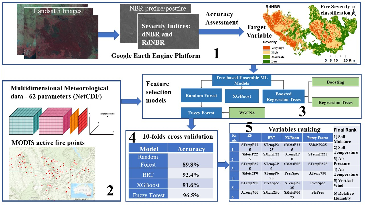
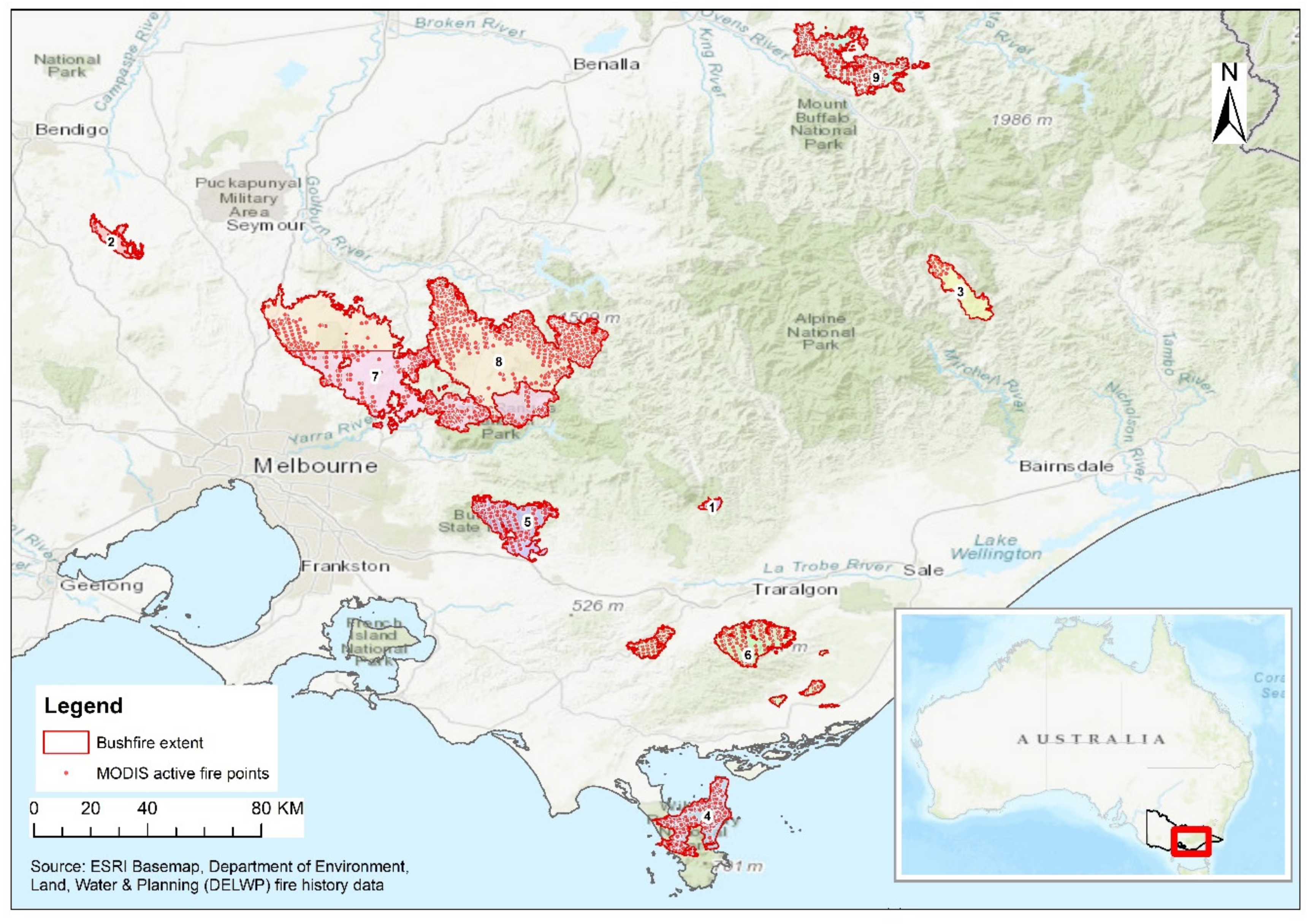
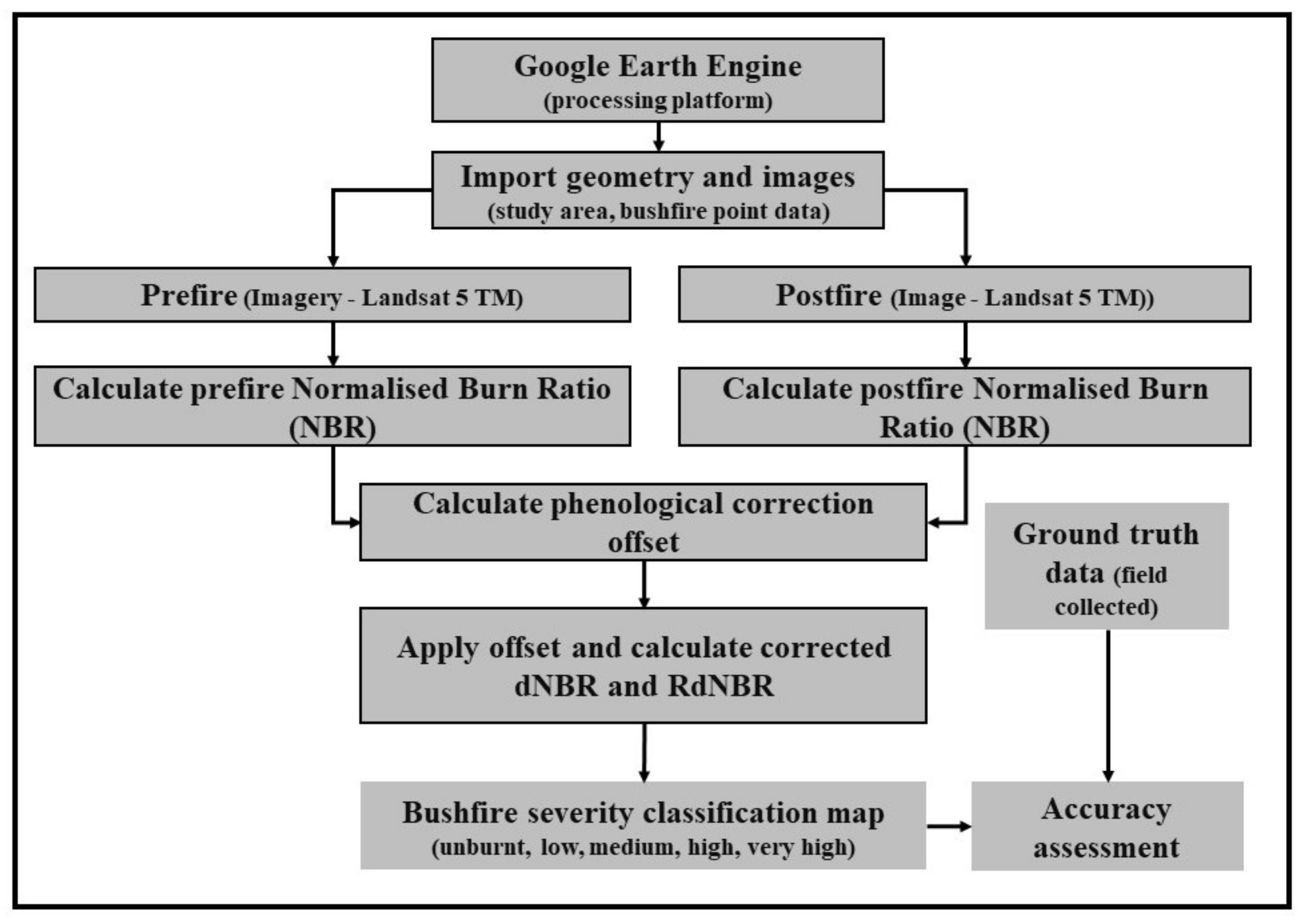
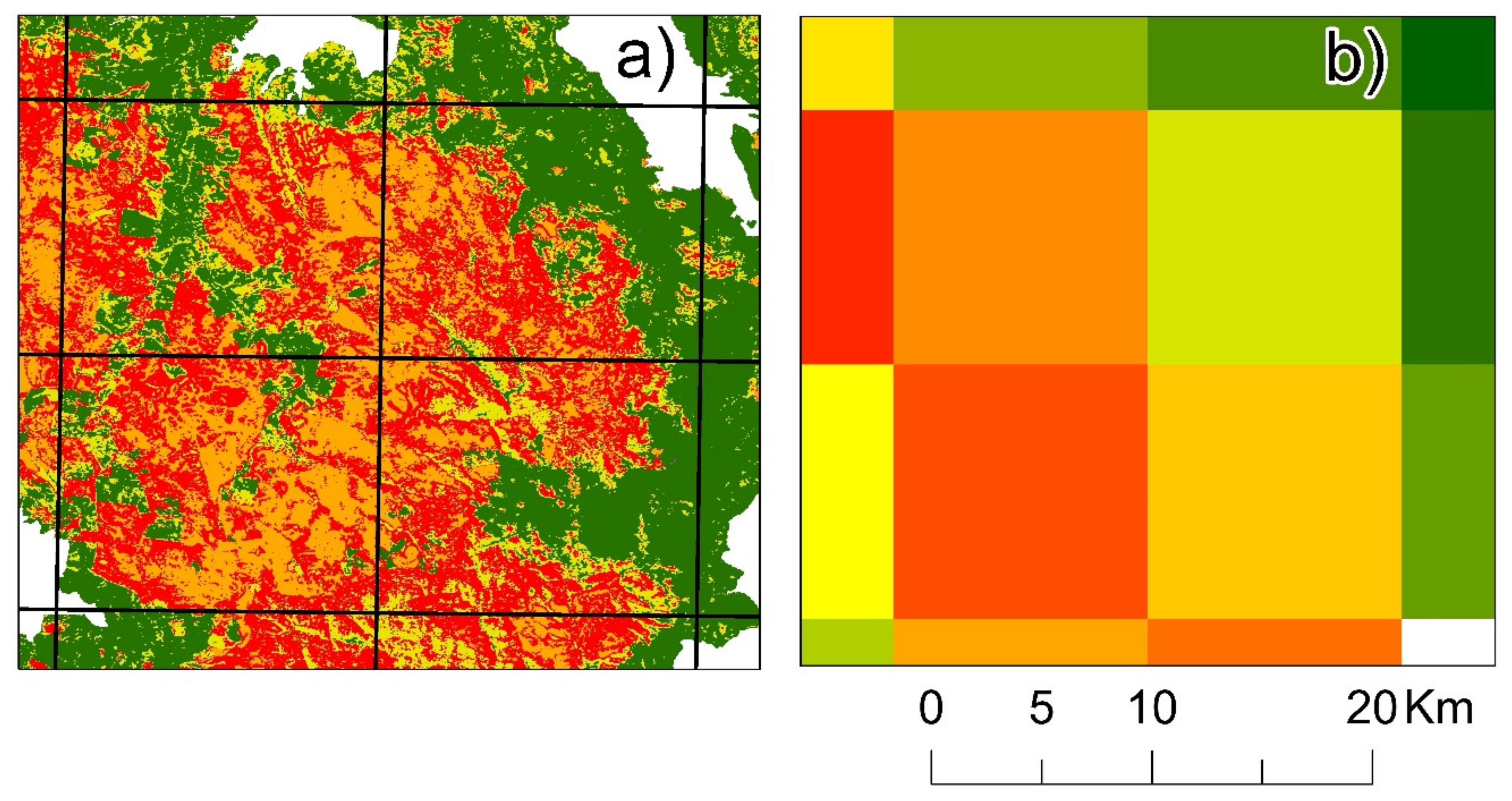
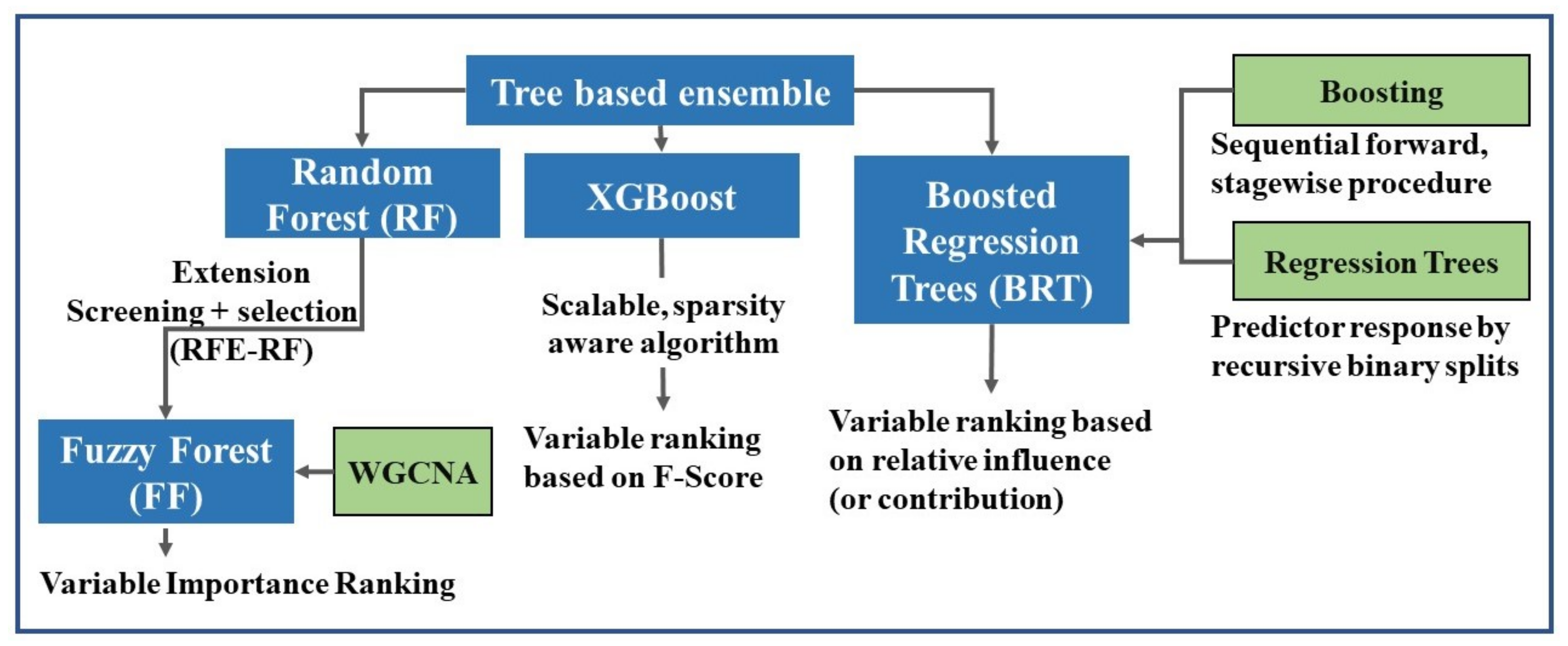
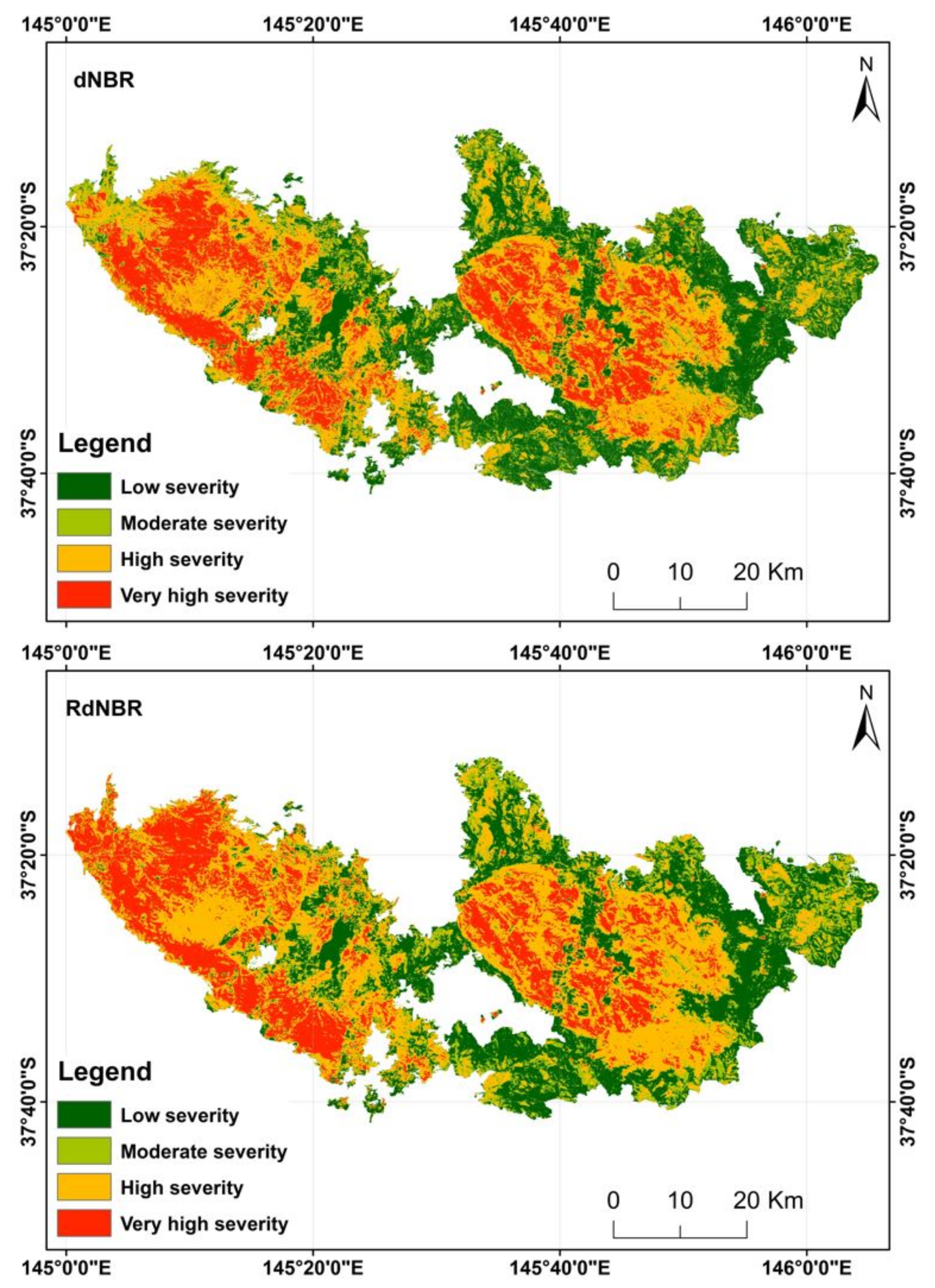
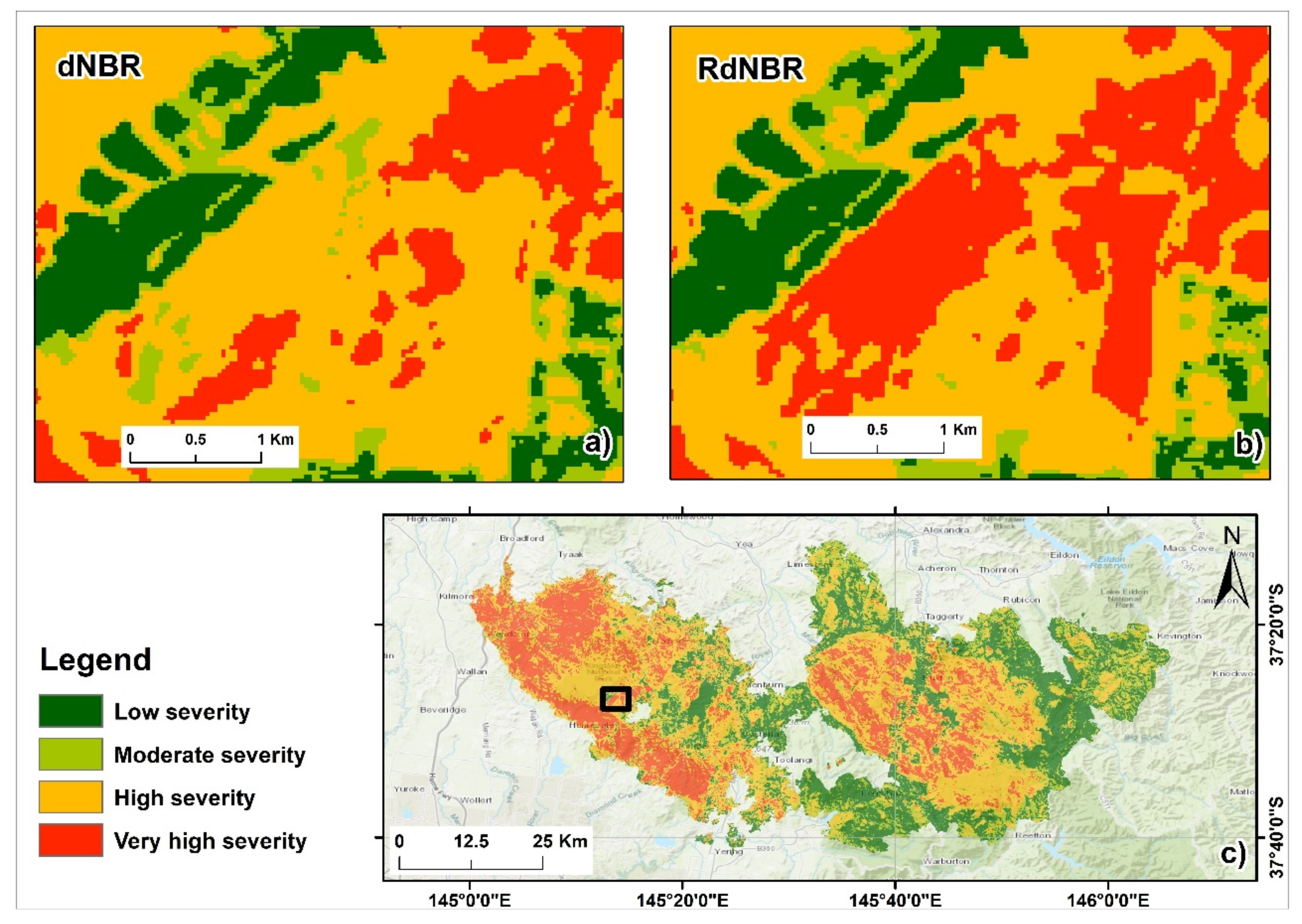
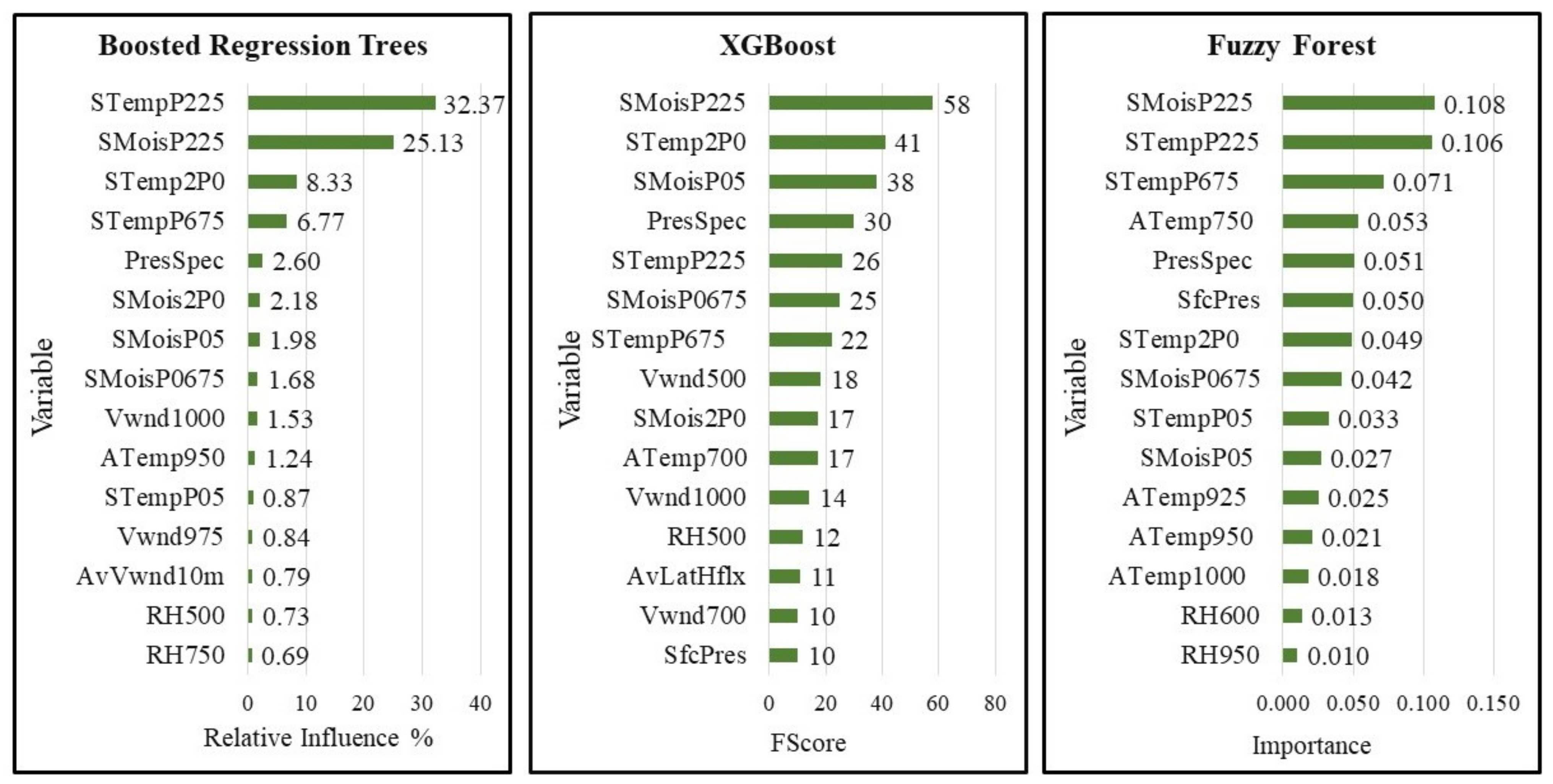
Table 1.
List of meteorological variables and parameters included in the analysis. The level column represents the number of vertical levels data collected. Single-level (S) data are measured at 1.5 m (unless specified otherwise). Multilevel data (M) represent 11 vertical levels determined by pressure isobars (1000 hPa, 975 hPa, 950 hPa, 925 hPa, 900 hPa, 850 hPa, 800 hPa, 750 hPA, 700 hPa, 600 hPa, 500 hPa) and multidepth data (D) include measurements from 4 different depth levels (0.05 m, 0.225 m, 0.675 m, and 2 m).
| Variable | Parameter | Data name | Level | Unit |
|---|---|---|---|---|
| Humidity | 6-hourly average of hourly mean atmospheric specific humidity | AvQsair | S | Kg kg−1 |
| 6-hourly average of instantaneous 10 min specific humidity | QsairScrn | S | Kg kg−1 | |
| 6-hourly average of hourly instantaneous relative humidity | RelHumPrs | M | % | |
| 6-hourly average of instantaneous specific humidity at the end of the hourly timestep | SpecHum | S | Kg kg−1 | |
| Moisture | 6-hourly average of hourly instantaneous soil moisture | SoilMois | D | Kg m−2 |
| Precipitation | Total precipitation amount at the surface | AccPrcp | S | Kg m−2 |
| Pressure | 6-hourly average of hourly mean air pressure | AvMslp | S | Pa |
| 6-hourly average of instantaneous 10 min air pressure | MslpSpec | S | Pa | |
| 6-hourly average of instantaneous 10 min air pressure at 20 m height | PresSpec | S | Pa | |
| Surface pressure at the end of the timestep | SfcPres | S | Pa | |
| Temperature | 6-hourly average of hourly instantaneous air temperature (multi-levels) | AirTemp | M | Kelvin |
| 6-hourly average of hourly maximum temperature | MaxTemp | S | Kelvin | |
| 6-hourly average of hourly minimum temperature | MinTemp | S | Kelvin | |
| 6-hourly average of instantaneous 10 min surface temperature (topsoil layer) at the end of the timestep | SfcTemp | S | Kelvin | |
| 6-hourly average of hourly instantaneous soil temperature (multidepth) | SoilTemp | D | Kelvin | |
| 6-hourly average of instantaneous 10 min temperature at 1.5 m | TempScrn | S | Kelvin | |
| Surface Flux | 6-hourly average of hourly mean surface upward latent heat flux | AvLatHflx | S | Wm−2 |
| 6-hourly average of hourly mean surface upward sensible heat flux | AvSenHflx | S | Wm−2 | |
| 6-hourly average of hourly instantaneous surface upward total moisture flux | AvSfc | S | kg m−2 s−1 | |
| Wind | 6-hourly average of hourly mean of wind U component at 10 m | AvUwnd10 m | S | ms−1 |
| 6-hourly average of hourly mean of wind V component at 10 m | AvVwnd10 m | S | ms−1 | |
| 6-hourly average of hourly mean of wind speed of gust at 10 m | WndGst10 m | S | ms−1 | |
| 6-hourly average of instantaneous 10 min U component of wind at 10 m | Uwnd10 m | S | ms−1 | |
| Upward air velocity (multilevel) | VwndPrs | M | ms−1 | |
| 6-hourly average of instantaneous 10 min V component of wind at 10 m | Vwnd10 m | S | ms−1 | |
| 6-hourly average of instantaneous 10 min wind speed of gust at 10 m | Wgust10 m | S | ms−1 |
Table 2.
Prefire and postfire Landsat 5 TM image tiles used for bushfire severity prediction of different fire events with different ignition dates under study.
Table 2.
Prefire and postfire Landsat 5 TM image tiles used for bushfire severity prediction of different fire events with different ignition dates under study.
| Fire Event | Fire Ignition Date | Acquisition Date (Prefire) | Acquisition Date (Postfire) |
|---|---|---|---|
| 1 | 7/02/2009 | 4/10/2008 | 23/10/2009 |
| 2 | 7/02/2009 | 3/11/2008 | 8/10/2010 |
| 3 | 6/02/2009 | 4/10/2008 | 23/10/2009 |
| 4 | 8/02/2009 | 4/10/2008 | 8/11/2009 |
| 5 | 4/02/2009 | 13/01/2008 | 1/12/2009 |
| 6 | 29/01/2009 | 4/10/2008 | 8/11/2009 |
| 7 | 7/02/2009 | 13/01/2008 | 1/12/2009 |
| 8 | 7/02/2009 | 13/01/2008 | 1/12/2009 |
| 9 | 7/02/2009 | 27/10/2008 | 30/10/2009 |
Table 3.
Burn severity category and classification threshold for dNBR and RdNBR raster layers. The class value of dNBR is scaled to 1000. The classification threshold was adopted from Cai and Wang (2020).
Table 3.
Burn severity category and classification threshold for dNBR and RdNBR raster layers. The class value of dNBR is scaled to 1000. The classification threshold was adopted from Cai and Wang (2020).
| Severity Category | Class Value (dNBR) | Class Value (RdNBR) |
|---|---|---|
| Unburnt | <100 | <0.1 |
| Low | 100–150 | 0.1–1.5 |
| Moderate | 150–250 | 1.5–2.5 |
| High | 250–350 | 2.5–3.5 |
| Very high | ≥350 | ≥3.5 |
Table 4.
Error matrices of bushfire severity classification for dNBR and RdNBR methods.
| Class (dNBR) | Very High | High | Moderate | Low | Total | User Accuracy | Kappa |
| Very High | 135 | 26 | 0 | 0 | 161 | 0.839 | |
| High | 14 | 208 | 2 | 4 | 228 | 0.912 | |
| Moderate | 0 | 1 | 35 | 22 | 58 | 0.603 | |
| Low | 0 | 1 | 13 | 159 | 173 | 0.919 | |
| Total | 149 | 236 | 50 | 185 | 620 | 0.000 | |
| Producer Accuracy | 0.906 | 0.881 | 0.700 | 0.859 | 0.000 | 0.866 | |
| Kappa | 0.811 | ||||||
| Class (RdNBR) | Very High | High | Moderate | Low | Total | User Accuracy | Kappa |
| Very High | 132 | 14 | 0 | 0 | 146 | 0.904 | |
| High | 17 | 220 | 2 | 3 | 242 | 0.909 | |
| Moderate | 0 | 1 | 44 | 19 | 64 | 0.688 | |
| Low | 0 | 1 | 4 | 163 | 168 | 0.970 | |
| Total | 149 | 236 | 50 | 185 | 620 | 0.000 | |
| Producer Accuracy | 0.886 | 0.932 | 0.880 | 0.881 | 0.000 | 0.902 | |
| Kappa | 0.861 |
Table 5.
Bushfire-influencing variables and their ranking obtained from different variable selection models. A brief explanation of the variables is presented in Table 1.
Table 5.
Bushfire-influencing variables and their ranking obtained from different variable selection models. A brief explanation of the variables is presented in Table 1.
| Rank | RF (VSURF) | Boosted Regression Trees | Fuzzy Forest | XGBoost | |||
|---|---|---|---|---|---|---|---|
| Variable | Variable | Relative Influence | Variable | Importance | Variable | F Score | |
| 1 | STempP225 | STempP225 | 32.37 | SMoisP225 | 0.108 | SMoisP225 | 58 |
| 2 | SMoisP225 | SMoisP225 | 25.13 | STempP225 | 0.106 | STemp2P0 | 41 |
| 3 | STempP675 | STemp2P0 | 8.33 | STempP675 | 0.071 | SMoisP05 | 38 |
| 4 | SMois2P0 | STempP675 | 6.77 | ATemp750 | 0.053 | PresSpec | 30 |
| 5 | STemp2P0 | PresSpec | 2.60 | PresSpec | 0.051 | STempP225 | 26 |
| 6 | ATemp700 | SMois2P0 | 2.18 | SfcPres | 0.050 | SMoisP0675 | 25 |
| 7 | SfcPres | SMoisP05 | 1.98 | STemp2P0 | 0.049 | STempP675 | 22 |
| 8 | PresSpec | SMoisP0675 | 1.68 | SMoisP0675 | 0.042 | Vwnd500 | 18 |
| 9 | SMoisP0675 | Vwnd1000 | 1.53 | STempP05 | 0.033 | ATemp700 | 17 |
| 10 | ATemp750 | ATemp950 | 1.24 | SMoisP05 | 0.027 | SMois2P0 | 17 |
| 11 | ATemp950 | STempP05 | 0.87 | ATemp925 | 0.025 | Vwnd1000 | 14 |
| 12 | STempP05 | Vwnd975 | 0.84 | ATemp950 | 0.021 | RH500 | 12 |
| 13 | SMoisP05 | AvVwnd10m | 0.79 | ATemp1000 | 0.018 | AvLatHflx | 11 |
| 14 | RH700 | RH500 | 0.73 | RH600 | 0.013 | SfcPres | 10 |
| 15 | Vwnd1000 | RH750 | 0.69 | RH950 | 0.010 | Vwnd700 | 10 |
Publisher’s Note: MDPI stays neutral with regard to jurisdictional claims in published maps and institutional affiliations. |
© 2022 by the authors. Licensee MDPI, Basel, Switzerland. This article is an open access article distributed under the terms and conditions of the Creative Commons Attribution (CC BY) license (https://creativecommons.org/licenses/by/4.0/).
Share and Cite
MDPI and ACS Style
Sharma, S.K.; Aryal, J.; Rajabifard, A. Remote Sensing and Meteorological Data Fusion in Predicting Bushfire Severity: A Case Study from Victoria, Australia. Remote Sens. 2022, 14, 1645. https://doi.org/10.3390/rs14071645
AMA Style
Sharma SK, Aryal J, Rajabifard A. Remote Sensing and Meteorological Data Fusion in Predicting Bushfire Severity: A Case Study from Victoria, Australia. Remote Sensing. 2022; 14(7):1645. https://doi.org/10.3390/rs14071645
Chicago/Turabian StyleSharma, Saroj Kumar, Jagannath Aryal, and Abbas Rajabifard. 2022. "Remote Sensing and Meteorological Data Fusion in Predicting Bushfire Severity: A Case Study from Victoria, Australia" Remote Sensing 14, no. 7: 1645. https://doi.org/10.3390/rs14071645
Note that from the first issue of 2016, this journal uses article numbers instead of page numbers. See further details here.