Offshore Oil Platform Detection in Polarimetric SAR Images Using Level Set Segmentation of Limited Initial Region and Convolutional Neural Network

Abstract

Offshore oil platforms are difficult to detect due to the complex sea state, the sparseness of target distribution, and the similarity of targets with ships. In this paper, we propose an oil platform detection method in polarimetric synthetic aperture radar (PolSAR) images using level set segmentation of a limited initial region and a convolutional neural network (CNN). Firstly, to reduce the interference of sea clutter, the offshore strong scattering targets were initially detected by the generalized optimization of polarimetric contrast enhancement (GOPCE) detector. Secondly, to accurately locate the contour of targets and eliminate false alarms, the coarse results were refined using an improved level set segmentation method. An algorithm for splitting and merging the smallest enclosing circle (SMSEC) was proposed to cover the coarse results and obtain the initial level set function. Finally, the LeNet-5 CNN model was used to classify the oil platforms and ships. Experimental results using multiple sets of polarimetric SAR data acquired by RADARSAT-2 show that the performance of the proposed method, including the detection rate, the false alarm rate, and the Intersection over Union (IOU) index between the extracted ROI and the ground truth, is better than the performance of a method that combines a GOPCE detector and a support vector machine classifier.

1. Introduction

The automatic detection and recognition of offshore targets is one of the most important problems in remote sensing image interpretation. It is widely used in applications such as navigation, marine monitoring, disaster prevention and reduction, maritime search and rescue, and safeguarding marine rights and interests [1]. The detection of offshore oil platforms is of great significance for the safe exploitation of offshore oil and gas and platform oil spill monitoring [2,3]. In PolSAR images, the scattering intensity of the offshore oil platform is high because of the double-bounce scattering components generated by the complex metal structure. Thus, the regions of interest (ROIs) of the offshore oil platform can be extracted by determining the high-intensity regions using the traditional constant false alarm rate (CFAR) method similarly as ship detection. However, it is difficult to detect the oil platform accurately due to the complex sea state, the sparse distribution characteristics of the target, and the similarity of targets with ships.

Since offshore oil platforms and ships are both metallic targets with similar superstructures, the scattering characteristics of oil platforms are almost the same as those of ships in SAR images. Therefore, various ship detection methods can also be used for the detection of offshore oil platforms. At present, there are mainly three kinds of ship detection methods: methods based on the CFAR detection of point targets, methods based on region segmentation, and methods based on deep neural networks.

The CFAR detection method includes four basic steps: scattering feature parameters extraction, sea clutter modeling, clutter sample censoring, and detection threshold determination. With respect to clutter modeling, the CFAR detection of polarimetric SAR images can be classified as a detector based on the hypothesis of a homogeneous region using the complex Wishart distribution [4], and as a detector based on the hypothesis of a heterogeneous region using the K distribution [5] and the G0 distribution [6]. From the perspective of clutter sample censoring, the CFAR detector has gone through development as the cell-averaging CFAR, the smallest-cell CFAR, and the order-statistics CFAR detector [7]. Cui et al. [8] and the authors in [9] proposed CFAR detection methods based on iterative sample censoring. Starting from the extraction of scattering parameters, the classic detectors in polarimetric SAR images include polarization whitening filter (PWF) [10], optimal polarimetric detector (OPD), polarimetric total power, and power maximum synthesis (PMS) detector [7]. Touzi et al. [11] proposed a ship detector using the parameters of polarization reflection symmetry, and validated the performance using Canadian airborne polarimetric SAR data under different incident angles and different polarization modes. Besides that, Chen et al. [12] proposed a ship detection method based on polarization cross-entropy. Yang et al. [13] proposed a ship detector based on the parameter of generalized optimization of polarimetric contrast enhancement (GOPCE). Touzi et al. [14] proposed a detector based on polarization degree. All the existing CFAR methods are pixel-based, with their performance depending on accurate clutter modeling and the construction of a detection window. In the case of rough sea states, there will be many false alarms and missing detections due to the interference of sea clutter and the weak scattering parts in the middle of the target. It is also difficult to extract the contour of the target because of the isolated strong scattering pixels and the broken detection region.

Different from the methods of pixel-based CFAR detection, the region-based segmentation methods segment the image into strong scattering and low scattering regions based on the scattering similarity of adjacent pixels. Lombardo et al. [15] and Renga et al. [16] pointed out that the false alarm rate of ship detection can be effectively reduced by segmentation. The region-based segmentation method mainly depends on two aspects: the model of the region’s statistical distribution and the model of the region’s boundary. With respect to the distribution model, the segmentation methods of polarimetric SAR images can be classified as models based on Wishart, G0, Kummer-U, and mixture Wishart distributions, and so on. With respect to the region boundary model, the segmentation models can be classified into region merged, Markov random field (MRF), and level set methods, and so on. On the assumption that the data obey a complex Wishart distribution, Yu et al. [17] proposed a region merged method based on the likelihood ratio distance of the coherent matrix. Rignot et al. [18] proposed an MRF segmentation method by building the spatial constraint of adjacent pixels. Ayed et al. [19] proposed a region-based level set segmentation by implicitly embedding the contour into a high-dimensional level set function. Liu et al. [20,21] proposed a hierarchical level set segmentation to segment the sea and land. Jin et al. [22] improved the level set model by assuming that the data obey the Kummer-U model. Since the models are region-based, an accurate contour of the targets can be obtained. However, those region-based segmentation methods are all sensitive to the initial segmentation. The segmentation is prone to converge to the local optimum in the case of random initialization.

Unlike the above pixel-based and region-based methods, which represent the data based on the statistical distribution of intensity or polarimetric parameters, deep neural networks build a full representation of tensor data by complex network structure. Lecun et al. [23] first proposed the convolutional neural network (CNN) model to recognize handwritten digits. Alex et al. [24] modified the pooling layer and activation function, and proposed a deep CNN model named AlexNet for large-scale image parallel operations. Subsequently, the CNN model has been continuously optimized—from VGG [25] and ResNet [26] to the recent SENet [27] model, the image classification performance has been continuously improved. As for the target detection method, from the earliest R-CNN [28] model to the later Fast/Faster R-CNN [29] and then the latest Yolo [30] and other models, the network structure has undergone changes from two stages to one stage, from a single-scale network to a feature pyramid network, and the performance of detection has been continuously improved. Ai et al. [31] proposed a ship detection method combining multi-scale rotation-invariant Haar-like features and CNN feature vectors. Jin et al. [32] used a deep CNN model based on patch-to-pixel for the detection of small ships. Zhao et al. [33] used the attention receptive pyramid network for ship detection in SAR images. However, when the deep neural network model was used in the detection of polarimetric SAR targets, it was difficult to collect sufficient training samples and extract the ROI under complex sea states in SAR images.

Although offshore oil platforms can be detected using ship detection methods, these methods cannot be directly used for offshore oil platform detection. In one respect, although the scattering characteristics of oil platforms and ships are almost the same, the oil platforms are usually sparsely distributed while ships are densely distributed. When extracting the ROI of oil platforms using the three kinds of ship detection methods mentioned before, the segmentation algorithm will be hard to converge. In another respect, the detected ROIs may include both ships and oil platforms. It is difficult to identify the oil platform targets from the extracted ROIs because the scattering characteristics and geometric structure of the targets are similar to those of ships. Thus, Chen et al. [34] proposed an oil platform detection method based on multi-temporal SAR images. Liu et al. [1] proposed an oil platform detection method based on multi-temporal Landsat-8 images. However, these multi-temporal methods cannot be used for single-phase images. Zhang et al. [35] proposed an oil platform detection method based on polarimetric parameters extracted from compact PolSAR data. Marino et al. [36] studied the multi-polarization characteristics of oil platforms using dual-polarization X-band SAR imagery. Migliaccio et al. [37] and Nunziata et al. [38] detected man-made metallic targets at sea using the reflection symmetry of quad-polarization data. However, the differences of these polarimetric parameters between oil platforms and ships are so small that it is difficult to extract oil platforms from the detected man-made metallic targets. Zhang and Wang et al. proposed using Hough transform [39] and neighborhood analysis [40] to eliminate the ship targets from the extracted ROIs. However, the classification accuracies of those geometric feature-based methods are insufficient since the differences in the geometric structure between the two kinds targets are small.

As a summary of the state of the art of offshore target detection with polarimetric SAR images, polarimetric parameters enhancing the contrast between the targets and the sea clutter need to be extracted first to reduce the interference of the sea clutter. The contour of the target can then be fixed by the region-based segmentation method. Finally, the oil platforms and ships can be classified using a deep neural network. Thus, a method of offshore oil platform detection in polarimetric SAR images based on the level set segmentation of a limited initial region and a CNN is proposed in this paper.

The main contribution of the work can be summarized as follows:

• Unlike the traditional pixel-based CFAR detection method, the level set segmentation method based on the CFAR detector of the polarimetric parameter of GOPCE is proposed for detecting offshore oil platforms and locating the contour of targets.
• Since the level set segmentation initialized by random circles is difficult to converge due to the sparse distribution characteristics of the target, an algorithm of splitting and merging the smallest enclosing circle (SMSEC) is proposed to initialize the level set function.
• Based on the ROI extraction and the feature selection of input data, the classic LeNet-5 model is used for the classification of offshore oil platforms and ships.

The rest of this paper is organized as follows. In Section 2, the method basis, including the level set segmentation and GOPCE detector, is briefly introduced. In Section 3, the proposed method is introduced in detail. Experimental results are shown and discussed in Section 4. The discussion is given in Section 5. The conclusion is given in Section 6.

2. Method Basis

2.1. Level Set Segmentation

To extract the ROI of an oil platform, a two-region level set segmentation method was used. In the method, the objective of the segmentation is to search for the optimum value of a defined energy function related to the segmentation curve. For the segmentation of two regions, if the image plane is $\mathbf{R}$, the given polarimetric SAR image is $\mathit{T}$, the segmentation boundary is represented as a curve $\mathsf{\Gamma }$, and the two regions divided by the curve $\mathsf{\Gamma }$ are ${\mathbf{R}}_1$ and ${\mathbf{R}}_2$. If the curve $\mathsf{\Gamma }$ is implicitly embedded in a level set function $\Phi \left(x,y,t\right)$, in which the zero level set function corresponds to the segmentation curve $\mathsf{\Gamma }\left(t\right)=\left\{\left(x\left(t\right),y\left(t\right)\right)|\Phi \left(x,y,t\right)=0\right\}$, then the objective energy function related to the level set function $\Phi$ can be defined as follows [41]:

$$E\left(\Phi \right)=\nu {\int }_{\mathbf{R}}\left|\nabla H\left(\Phi \right)\right|dR-{\int }_{\mathbf{R}}H\left(\Phi \right)lnf\left(\mathit{T}|{\mathbf{R}}_1\right)+\left(1-H\left(\Phi \right)\right)lnf\left(\mathit{T}|{\mathbf{R}}_2\right)dR,$$

(1)

where $H\left(\Phi \right)$ is the step function, and ∇ denotes the gradient. When $\Phi \ge 0$, $H\left(\Phi \right)=1$, and $\Phi <0$, $H\left(\Phi \right)=0$. ${\mathbf{R}}_1$ corresponds to $\Phi \ge 0$ and ${\mathbf{R}}_2$ corresponds to $\Phi <0$. $f\left(\mathit{T}|{\mathbf{R}}_i\right)\left(i=1,2\right)$ denotes the probability density function of region ${\mathbf{R}}_i$. The first item of $E\left(\Phi \right)$ denotes the internal energy which restricts the length of the segmentation curve, while the second item of $E\left(\Phi \right)$ denotes the external energy related to the zero level set function.

According to the Euler–Lagrange equation, to search the optimum value of the objective function, the energy function needs to change along the derivative of the level set function with respect to time [41]:

$$\frac{\partial \Phi }{\partial t}=-\left|\nabla \Phi \right|F\left(\mathit{T}\right)=-\left|\nabla \Phi \right|\left(\nu \kappa +ln\frac{f\left(\mathit{T}|{\mathbf{R}}_2\right)}{f\left(\mathit{T}|{\mathbf{R}}_1\right)}\right),$$

(2)

where the curvature of the curve $\kappa =-div\left(\nabla \Phi /\left|\nabla \Phi \right|\right)$, $div\left(·\right)$ is the divergence, $\nu$ is the regularization parameter of the curve, and $F\left(\mathit{T}\right)$ is the speed of evolution.

The scattering matrix of each homogeneous region of the multi-look polarimetric SAR image obeys the complex Wishart distribution. If the average coherent matrix of the region is $\mathsf{\Sigma }$ and the number of looks is L, then its coherent matrix $\mathit{T}\sim W\left(\mathsf{\Sigma },L,p\right)$

$$f\left(\mathit{T}|\mathsf{\Sigma },L,p\right)=\frac{L^{pL}{\left|\mathit{T}\right|}^{L-p}\exp \left\{-L\mathrm{tr}\left({\mathsf{\Sigma }}^{-\mathbf{1}}\mathit{T}\right)\right\}}{{K\left(L,p\right)\left|\mathsf{\Sigma }\right|}^L},$$

(3)

where p is the number of polarization channels, $\mathrm{tr}\left(·\right)$ is the trace of the matrix, $K\left(L,p\right)={\pi }^{\frac{p\left(p-1\right)}{2}}\mathsf{\Gamma }\left(L\right)\dots \mathsf{\Gamma }\left(L-p+1\right)$, and $\mathsf{\Gamma }\left(·\right)$ is the Gamma function.

According to Equations (2) and (3), if the average coherent matrices of two regions after segmentation are ${\mathsf{\Sigma }}_{\mathbf{1}}$ and ${\mathsf{\Sigma }}_{\mathbf{2}}$, respectively, then the level set evolution speed function is:

$$F\left(\mathit{T}\right)=\nu \kappa +L\left(\ln \left({\mathsf{\Sigma }}_1\right)+\mathrm{tr}\left({{\mathsf{\Sigma }}_1}^{-1}\mathit{T}\right)\right)-L\left(\ln \left({\mathsf{\Sigma }}_2\right)+\mathrm{tr}\left({{\mathsf{\Sigma }}_2}^{-1}\mathit{T}\right)\right),$$

(4)

where ${\mathsf{\Sigma }}_{\mathbf{1}}$ and ${\mathsf{\Sigma }}_{\mathbf{2}}$ are estimated in each iteration according to the inner and outer regions of the temporal zero level set function.

$${\mathsf{\Sigma }}_i^{\left(t+1\right)}=\frac{1}{N_i^{\left(t\right)}}\sum _{\left(x,y\right)\in {\mathbf{R}}_i^{\left(t\right)}}\mathit{T}\left(x,y\right),$$

(5)

where t denotes the t-th iteration, $\mathit{T}\left(x,y\right)$ denotes the coherent matrix of point $\left(x,y\right)$, and $N_i$ denotes the number of pixels of region ${\mathbf{R}}_i$.

From Equations (4) and (5), we can see that $F\left(\mathit{T}\right)$ is close to zero when the difference between ${\mathsf{\Sigma }}_{\mathbf{1}}$ and ${\mathsf{\Sigma }}_{\mathbf{2}}$ is small.

With a setting initial level set function $\Phi$ and parameter value $\nu$, the segmentation of land and water can be carried out by iteratively evolving the level set function using Equations (4) and (5).

2.2. GOPCE Detector

To obtain an initial detection of the ROIs of an oil platform, a GOPCE detector was used. Let A denote the target and B the background. Suppose the average Kenaugh matrix of A is ${\mathit{K}}_A$ and that of B is ${\mathit{K}}_B$; furthermore, suppose that $\mathit{g}={\left(1,g_1,g_2,g_3\right)}^t$ and $\mathit{h}={\left(1,h_1,h_2,h_3\right)}^t$ are the two optimal polarization states, $\mathit{r}={\left(r_1,r_2,r_3\right)}^t$ are the three general parameters, $r_1$ denotes the similarity parameter between the target and a plane, $r_2$ denotes the similarity parameter between the target and a dihedral, and $r_3$ denotes the Cloude entropy [42]. The GOPCE detector can then be defined as follows [13]:

$$\begin{array}{cc}\hfill Maximize& \frac{\frac{1}{M}{\sum }_A{\left[{\sum }_{i=1}^3{x}_i{r}_i\left(A\right)\right]}^2}{\frac{1}{N}{\sum }_B{\left[{\sum }_{i=1}^3{x}_i{r}_i\left(B\right)\right]}^2}\times \frac{{\mathit{h}}^t{\mathit{K}}_A\mathit{g}}{{{\mathit{h}}^t\mathit{K}}_B\mathit{g}}\hfill \\ \hfill Subjectto& g_1^2+g_2^2+g_3^2=1\hfill \\ \hfill & h_1^2+h_2^2+h_3^2=1\hfill \\ \hfill & x_1^2+x_2^2+x_3^2=1\hfill \end{array}$$

(6)

where $\mathit{x}={\left(x_1,x_2,x_3\right)}^t$ are three coefficients of parameters $\mathit{r}$.

3. The Proposed Method

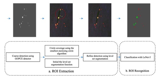
The algorithm flow of the proposed method is shown in Figure 1. In the ROI extraction step, a level set segmentation algorithm initialized by the GOPCE detector (GOPCE-LS) is proposed for extracting the ROIs from coarse to fine. Offshore strong scattering targets are coarsely detected using the GOPCE detector first. All the coarse detected targets are then covered with multiple circles using the smallest circle enclosing algorithm. The level set function is initialized by the circles. The ROIs of the offshore oil platform are finally extracted using the improved level set segmentation. In the ROI recognition step, oil platforms are recognized from the extracted ROIs using the classic LeNet-5 model.

3.1. Initialization of Level Set Segmentation

To accurately extract the ROIs of strong scattering targets on the sea using level set segmentation, an initial level set function needs to be defined. As shown in the mesh grid in Figure 2, we usually defined the initial level set function as a signed distance function (SDF), which takes the circle in the image center as the initial segmentation curve and takes the distance between the pixel and the circle center as the initial level set function. If $\left(x_c,y_c\right)$ is the center of the image and the setting radius of the circle is $r_c$, then the initial level set function can be represented as follows:

$${\Phi }^0\left(x,y\right)=2Aexp\left\{-D\left({\left(x-x_c\right)}^2+{\left(y-y_c\right)}^2\right)\right\}-A,$$

(7)

where A and D are constants, and $D=\frac{1}{r_c^2}ln2$ is to keep ${\Phi }^0$ equal to zero on the points of the boundary circle.

In Figure 2, the center $\left(x_c,y_c\right)$ is $\left(0,0\right)$, $r_c^2$ equals 8, and A is set to 5. The green plane is the zero plane. The intersection circle between the SDF and the zero plane denotes the zero level set function.

When the image-centered circle or a random circle is used for the initialization, the inner region of the circle denotes the region where the level set function is greater than zero, while the outside is smaller than zero, as shown in Figure 3a. In Figure 3, the rectangle denotes the image plane, the spots drawn in red denote targets, and the blue circle denotes the initial zero level set function. However, there may be some targets inside the circle and some targets outside the circle, as shown in Figure 3b. If the total area of the targets inside the circle is close to that of the outside region, the average coherent matrix of the inner region ${\mathsf{\Sigma }}_1$ is almost equal to that of the outside region ${\mathsf{\Sigma }}_2$. The evolution speed of the level set segmentation (4) is so close to zero that the algorithm is difficult to converge.

To avoid the problem of slow convergence caused by the initialization with a single circle, a straightforward alternative plan is to compute the initial SDF using multiple circles rather than a single circle. As shown in Figure 3c, the image is divided into multiple square regions at equal intervals, in each of which a circle for initialization is extracted. If the coordinate of the center of one sub-region is $\left(x_i,y_i\right)$ and the radius of the circular is $p_i$, where $\left(i=1,\dots ,N_p\right)$ and $N_p$ is the number of sub-regions, then the initial level set function is:

$${\Phi }^0\left(x,y\right)=2Aexp\left\{-D_l\underset{i}{min}\left({\left(x-x_i\right)}^2+{\left(y-y_i\right)}^2\right)\right\}-A,$$

(8)

where $D_i=\frac{1}{{p_i}^2}ln2$ and $l={\mathrm{argmin}}_i\left({\left(x-x_i\right)}^2+{\left(y-y_i\right)}^2\right)$.

However, the slow convergence problem still exists in some cases. Supposing that there is a single small target, that half of the target is in a circle, and that the other half is outside the circle, as shown in Figure 3d, the evolution speed of the level set will also be close to zero since the average coherent matrix of the inner and outer regions of the initial segmentation curve is almost equal.

To further avoid the slow convergence problem, it is necessary to define a more reasonable initial segmentation curve. If we know the coarse position of the targets, we can initialize the level set function according to the boundary of the coarse result. However, the level set function cannot be initialized by a curve of any shape obtained by the boundary of the coarse result. Thus, we propose covering the coarsely detected targets using multiple circles based on the position distribution of the target regions. If the initial circles are close to the true boundary of the targets, the above half-coverage problem can be avoided.

3.2. Coarse Detection of Targets

To initialize the level set function using multiple circles, an initial detection of the suspicious targets is needed first. In an SAR image, the double-bounce scattering component between the tightly connected metal structure makes the oil platform constitute a strong scatterer. As shown in Figure 4, a Pauli pseudo-color image of oil platforms on the coast of Singapore is shown in Figure 4a. The corresponding ground truth is shown in Figure 4b, where the region marked by the red box is the oil platform. We can observe that the targets appear as a white light area with irregular contours. Thus, the initial detection can be fulfilled using the general CFAR detection method of strong scattering targets. However, accurate clutter modeling, sample censoring and detection window construction are needed in the case of a high sea state. Since only a coarse result is needed for the initial detection, the detection can be improved by extracting the polarimetric parameters of the targets. In polarimetric SAR images, the scattering component of the oil platform is complex due to the complex metal structure. Firstly, the similarity of the scattering matrix between the targets and a dihedral is high because of the double-bounce scattering component. Secondly, the polarimetric entropy and alpha angle is high according to the $H/\alpha$ classification plane [42] since the targets can be classified in the high-entropy double-bounce scattering region. Finally, the contrast of the double-bounce similarity and the polarimetric entropy between the targets and the background is high. The GOPCE detector can enhance the contrast of similarity parameters and polarimetric entropy between targets and background in a combination of the selection of an optimal polarization state. Since the contrast is greatly enhanced, the target pixels can be simply detected by a global thresholding of the GOPCE parameter. Therefore, the GOPCE detector (6) performing in a thresholding of a single pixel without sliding window construction was used for the detection of the oil platform.

3.3. Circle Calculation

When the coarse results of targets are detected, a circle covering all the detected targets needs to be computed to initialize the level set function using SDF. Since a smaller covered circle means a larger distance of the coherent matrix between the inner and outer segmentation regions, which is better for the convergence of segmentation, we need to find the smallest enclosing circle. As shown in Figure 5, the white region in the rectangle denotes the sea and the red spot denotes the detection targets. Three detected targets are covered by a single circle in Figure 5a, which is the smallest enclosing circle since the circle is just a coverage of the targets.

If the set of pixel coordinates of the initial detected targets is ${\left\{P_i=\left(x_i,y_i\right)\right\}}_{i=1}^N$, where N is the total number of target pixels, then the problem can be described as “Given N points on a plane, cover all the points with a circle, and find the center and radius of the circle”. The problem can be solved by the incremental method [43]. The specific algorithm steps are as follows (Algorithm 1).

Algorithm 1 The smallest enclosing circle algorithm (Circle C) = Smallest_circle(Points${\left\{P_i\right\}}_{i=1}^N$)

1: Initialization: select two points $\left(P_1,P_2\right)$, consider $P_2$ as the current point, and obtain the initial circle $C_2$ with diameter $P_1{P}_2$ (the circle determined by point $P_i$ is $C_i$); 2: $i=3$, then for each $P_i$, if $P_i$ is inside $C_{i-1}$, then $C_i=C_{i-1}$; otherwise go to step 3; 3: Construct a new circle containing $P_i$. First determine $C_i^0$ with diameter $P_1{P}_i$, if points $P_1{\dots P}_{i-1}$ are all inside $C_i^0$, then $C_i=C_i^0$; otherwise go to step 4; 4: If there is a point $P_j\left(j<i\right)$ which is not in $C_i^0$, obtain a new circle $C_i^1$ with diameter $P_i{P}_j$. If points $P_1{\dots P}_{j-1}$ are all inside $C_i^1$, then $C_i=C_i^1$; otherwise go to step 5; 5: If there is a point $P_k\left(k<j<i\right)$ which is not in $C_i^1$, obtain a new circle $C_i^2$ with three points $\left(P_i,P_j,P_k\right)$, and finally $C_i=C_i^2$; 6: Repeat Steps 2–5 until $i=N$. Return $C_N$.

All target pixels can be covered by a circle using the smallest enclosing circle algorithm. However, the problem is that if the targets are scattered and distributed in the image, the calculated circle will be so large that the area of the sea in the covered circle is much larger than that of targets, as shown in Figure 5a. The distance of the coherent matrix between the inner and outer regions thus becomes smaller. Therefore, the scattered targets need to be classified into a group and covered with different circles, as shown in Figure 5b. To simplify the grouping process, a strategy of splitting and merging was taken, as shown in Figure 6. In the splitting step, the image plane is recursively split into small regions. Two splitting steps are shown in Figure 6. A region R is first equally divided into four phases $R_i(i=1,2,3,4)$. Each sub-region $R_i$ is then equally divided into phases $R_{ij}(j=1,2,3,4)$. In the merging step, the target pixels in a sub-region are covered by a circle using the smallest enclosing circle algorithm. The splitting and merging process continues until the size of sub-region is less than a constant value SC. Supposing $\mathbf{R}$ denotes the image plane and the size is $X\times Y$, to ensure that the size of the sub-region is not too large, the region is to be split if the diameter of the smallest enclosing circle of the target pixels in the region is greater than $min\left(X,Y\right)/4$ at the beginning of the algorithm. Then, for a given $Z\times Z$ region, if the diameter of the smallest enclosing circle of the region is greater than Z, the region will be split. Supposing the smallest size of the splitting region to be ${SC=2}^Q$, the algorithm can be described as follows (Algorithm 2).

Algorithm 2 Split and merge circle coverage algorithm Split_merge(region $\mathbf{R}$, xlabel u, ylabel v, size n)

1: if  $n==SC$  then 2:    if $\exists \left(u_0,v_0\right)s.t.\mathbf{R}\left(u_0,v_0\right)==1$ then 3:       $Cr\leftarrow (u+n/2,v+n/2,n/2)$  4:       return 5:    end if 6: else 7:    (center, radius) = Smallest_circle ($\mathbf{R}$, u, v, n) 8:    if $2radius\le 2^{(M-k)}\&\&2radius\le min(X,Y)/4$ then 9:       $Cr\leftarrow$(center(1), center(2), radius) 10:    else 11:       Split_merge($\mathbf{R}$, u, v, $n/2$)       Split_merge($\mathbf{R}$, $u+n/2$, v, $n/2$)       Split_merge($\mathbf{R}$, u, $v+n/2$, $n/2$)       Split_merge($\mathbf{R}$, $u+n/2$, $v+n/2$, $n/2$) 12:    end if 13: end if

In Algorithm 2, $\mathbf{R}$ denotes the segmented region, u and v are the coordinates of the left corner point of $\mathbf{R}$, n denotes the size of R, and $Cr$ denotes the set of circles. At the beginning of the algorithm, the $X\times Y$ image plane $\mathbf{R}$ is padded into $2^M\times 2^M$ with zero, where M is the minimum number such that $2^M$ is larger than X and Y. R is set to $\mathbf{R}$, u and v are set to 0, n is set to $2^M$, and $Cr$ is set to ∅.

If the center of the circle ${Cr}_j\left(j=1,\dots ,N_q\right)$ computed by Algorithm 2 is $\left(x_j,y_j\right)$ and the radius is $q_j$, we can obtain the final initial level set function as follows.

$${\Phi }^0\left(x,y\right)=2Aexp\left\{-D_l\underset{j}{min}\left({\left(x-x_j\right)}^2+{\left(y-y_j\right)}^2\right)\right\}-A,$$

(9)

where $D_j=\frac{1}{{q_j}^2}ln2$ and $l={\mathrm{argmin}}_i\left({\left(x-x_i\right)}^2+{\left(y-y_i\right)}^2\right)$.

3.4. ROI Extraction

Based on the initial level set function defined by Equation (9), the regions of strong scattering and low scattering can be segmented by evolving the level set function using Equation (10) based on Equation (4).

$$\Phi \left(t+\mathsf{\Delta }t\right)=\Phi \left(t\right)-\left|\nabla \Phi \right|F\left(\mathit{T}\right)\mathsf{\Delta }t$$

(10)

When the evolution is terminated, the strong scattering and low scattering regions can be identified by comparing the average power of the two segmented regions. The ROIs of the targets on the sea can be extracted by determining all the connected strong scattering regions from the segmentation result.

3.5. ROI Recognition

Supposing the extracted ROIs to be $\left\{{ROI}_i\right\}$, the final step of oil platform recognition is to classify $\left\{{ROI}_i\right\}$ into oil platforms and ships. Because the shape of oil platforms and ships is similar, it is difficult to accurately classify the two kinds of target using traditional geometric-based methods. Since deep network structure can fully represent data without geometric features extraction, CNN was taken as the classifier. Because the size of the ROI is small and the number of training samples was small, the lightweight CNN model LeNet-5 [23] was selected to perform the classification.

To use the CNN model, the input data and the network need to be constructed. Because the coherent matrix $\mathit{T}$ is a $3\times 3$ complex matrix, the nine elements need to be vectorized as the input. Since the difference of the scattering components between the oil platform and the ship is small and the main difference of the two targets is the contour shape, only the three diagonal elements $\left(T_{11},T_{22},T_{33}\right)$ of $\mathit{T}$ in a combination of the GOPCE parameter were selected as the input data.

The LeNet-5 model requires the input image to have a fixed size $J\times J$. However, the size of the extracted ROI varies. To avoid statistical distortion of the data caused by image zooming, we directly cropped a fixed $J\times J$ region in the center of the circumscribed rectangle of each ROI.

Since the dynamic range of the scattering power of the SAR image is large, the sigmoid activation function of the LeNet-5 model was replaced with the ReLU activation function, and the average pooling was replaced with maximum pooling in the polling layer. The network structure of the model is shown in

Table 1. The LeNet-5 network structure, where W denotes the weights of the unit and b denotes the bais of the unit.

Layer	Patch/Stride	Type	Output	Parameters
1	$5\times 5/1$	Convolution	$28\times 28\times 6$	W  $5\times 5\times 3\times 6$ b  $1\times 1\times 6$
2	$2\times 2/2$	Max Pooling	$14\times 14\times 6$	-
3	$5\times 5/1$	Convolution	$10\times 10\times 16$	W  $5\times 5\times 6\times 16$ b  $1\times 1\times 16$
4	$2\times 2/2$	Max Pooling	$5\times 5\times 16$	-
5	$5\times 5/1$	Convolution	$1\times 1\times 64$	W  $5\times 5\times 16\times 64$ b  $1\times 1\times 64$
6	-	Fully Connected	$1\times 1\times 32$	W  $32\times 64$ b  $32\times 1$
7	-	Fully Connected	$1\times 1\times 3$	W  $3\times 32$ b  $3\times 1$

. We also added a batch normalization layer after each convolutional layer and fully connected layer. The input was a 4-channel image of $32\times 32$. The output was a 3-dimensional vector representing three different categories of oil platform, ship, and background.

4. Experimental Results and Analysis

Seven single-look quad-polarization SAR datasets acquired by the RADARSAT-2 sensor over the coasts of Brunei, Ho Chi Minh City in Vietnam, El Nido in Philippines, and the Beibu Gulf of China were used to test the proposed method. The detailed parameters of the data are shown in

Table 2. Experimental dataset details, where UTC stands for the international standard time, AOI stands for the angle of incident of the center point of the image, and $\mathrm{m}\times \mathrm{m}$ stands for meter times meter.

Dataset	Scene	Size	Resolution $\mathrm{m}\times \mathrm{m}$	UTC	AOI $\left({}^{°}\right)$
1	Brunei	$5553\times 3789$	$4.73\times 5.14$	06/04/2012 22:03:48	40.91
2	Ho Chi Minh City	$5714\times 2888$	$4.73\times 5.18$	06/08/2012 10:56:07	30.01
3	EI Nido	$6173\times 4256$	$4.73\times 4.78$	06/08/2012 21:45:25	47.42
4	Beibu Gulf	$5733\times 4316$	$4.73\times 5.07$	06/20/2012 22:33:46	48.16
5	Brunei	$5723\times 4100$	$4.73\times 5.15$	06/09/2012 22:58:01	45.09
6	Ho Chi Minh City	$6159\times 4208$	$4.73\times 4.73$	06/11/2012 11:08:26	46.62
7	Beibu Gulf	$5670\times 3716$	$4.73\times 4.84$	06/13/2012 22:37:17	40.01

. The range resolutions were all $4.73\mathrm{m}$. The azimuth resolutions were varied from $4.78\mathrm{m}$ to $5.18\mathrm{m}$. The size of the images was about $6000\times 4000$. To evaluate the performance of the proposed method, we drew the ground truth of the oil platforms by referring first to Google Earth and artificial judgment. Dataset 1 was then taken as an example to show the flow of the proposed method in Experiment A. The validation of the proposed method was divided into three parts. The first part validated the robustness of the proposed method by testing the method using data from different sites in Experiment B. The second part validated the performance of the ROI extraction. In Experiment C, the detection performance of the proposed GOPCE-LS method was first compared with that of different CFAR detection methods. The performance of the proposed GOPCE-LS method was then compared under different level set initialization methods and different algorithm parameters in Experiment D. The third part validated the performance of the ROI recognition. The recognition performance of the proposed method was compared with that of the support vector machine (SVM) classifier based on the ROI extraction result of GOPCE-LS in Experiment E.

The performance was evaluated using detection rate, false alarm rate, and two Intersection over Union (IOU) indexes. The macro-IOU computed the IOU between the detected result and the ground truth independently for each target and then computed the average, whereas the micro-IOU aggregated the contribution of all targets to compute the average IOU metric. If the detected result is $DR=\left\{{DR}_i\right\}\left(i=1,\dots ,M\right)$ and ${DR}_i$ denotes the ith candidate target, and if the ground truth is $GT=\left\{{GT}_j\right\}\left(j=1,\dots ,N\right)$ and ${GT}_j$ denotes the jth true target, then the macro-IOU and micro-IOU are defined as follows:

$$\begin{array}{cc}\hfill & macro\text{-}IOU=\frac{1}{N}\sum _{j=1}^N\frac{{DR}_i\cap {GT}_j}{{DR}_i\cup {GT}_j},\hfill \\ \hfill & micro\text{-}IOU=\frac{DR\cap GT}{DR\cup GT},\hfill \end{array}$$

(11)

where $DR\cup GT$ denotes the union of the two sets, $DR\cap GT$ denotes the intersection of the two sets, and ${DR}_i\cap {GT}_j({DR}_i\cup {GT}_j)$ denotes the intersection (union) of the target ${GT}_j$ with the intersecting detected target ${DR}_i$.

In the experiment, the image was processed by $5\times 5$ multi-look processing to reduce the input size of the extracted ROI, where the size of the multi-look was determined by the average width and length of the oil platform and the input size of the CNN network model. In the coarse detection step, the probability of a false alarm (PFA) was set to 0.01. The strong scattering regions and the other regions in the ground truth were selected as the samples of target and background, respectively. When the splitting and merging algorithm was carried out, the minimum split size Q was set to 3, where Q can be set to 2–6. When performing the level set segmentation, the parameter A was set to 100, the curve parameter $\nu$ was set to 0.1 [20], and the maximum number of iterations was set to 200. Where the parameter PFA was set according to Experiment C, the parameters Q and $\nu$ were set according to Experiment D. For CNN classification, the input image size was set to $32\times 32$. When training the model, the batch size was set to 10, and the number of epochs was set to 20. In the experiment, parts of the seven datasets were randomly selected as training data, and the other datasets were used for testing. For performance analysis, we conducted the test using datasets 1–3 for training and datasets 4–7 for testing as examples. The testing platform used was Matlab v9.5 and CPU was Intel Xeon at 3.6 GHz with 16 GB RAM.

4.1. Results on Example Data

In the first experiment, Dataset 1 was taken as example data to show the detailed procedures of the proposed method. The Pauli pseudo-color image of the data is shown in Figure 7a. We can observe that several oil platforms surrounded by ships are sparsely distributed on the sea. It is difficult to distinguish oil platforms from ships because of their similar intensity and geometric structure. The coarse detected result of the ROI is shown in Figure 7b, where the white regions denote the detected targets and the gray regions denote the background. From the result we can find that almost all targets were correctly detected by the GOPCE detector. However, because H was calculated in a sliding window, there were some offsets between the extracted target contour and the actual contour. The circles obtained by the proposed split and merge smallest enclosing circle method are shown in Figure 7c, where the circles are drawn in red. The zooming result of Figure 7c near the island is shown in Figure 7d. We can find that all targets are correctly covered by multiple circles. The segmentation result is shown in Figure 7e, where the segmentation boundary is drawn in red. The zooming result of Figure 7e near the island is shown in Figure 7f. We can see that the segmentation boundary is accurately fixed in the actual boundary of the targets from Figure 7f. The result of the extracted ROIs is shown in Figure 7g, where the detected ROIs are marked in a red box. From Figure 7g, we can find that the sizes of the marked ROIs are varied. The final recognition result is shown in Figure 7h and the zooming result is shown in Figure 7i, where the detected oil platforms are drawn in green and the ships are drawn in red. We can observe that the oil platforms were correctly separated from ships by the CNN classifier. The detection accuracies, including detection rate, false alarm rate, and two IOU indexes, are listed in the second row of

Table 3. Performances of the proposed method under different sites, where Num denotes the number of targets, Pd denotes the detection rate, Pf denotes the false alarm rate, Nd denotes the number of correctly detected targets, Nf denotes the number of false alarms, Macro denotes the macro-IOU index, Micro denotes the micro-IOU index, and $\mathsf{\Sigma }$ denotes the overall performance.

Data	Num	Nd	Pd	Nf	Pf	Macro	Micro
1	6	6	100	0	0	0.9925	0.9927
2	6	6	100	0	0	0.9955	0.9954
3	2	2	100	0	0	0.9703	0.9593
4	5	5	100	0	0	0.9758	0.9785
5	5	5	100	0	0	0.9920	0.9917
6	5	5	100	0	0	0.9936	0.9927
7	7	7	100	0	0	0.9842	0.9662
$\mathbf{\Sigma }$	36	36	100	0	0	0.9863	0.9824

. All the six oil platforms in the data were correctly detected and the two IOU indexes were both higher than 99%.

4.2. Test under Different Sites

To validate the robustness of the method, the proposed method was tested using data from different sites. The result of Datasets 2–5 of Table 2 are shown in Figure 8, where the results of data $i+1$ are shown in Figure 8(a1–e1). The Pauli pseudo-color images of the data are shown in Figure 8(a1–a4). We can see that the oil platforms are all sparsely distributed. The coarse detected results of the ROI are shown in Figure 8(b1–b4). The circle coverage results are shown in Figure 8(c1–c4). The final detection results are shown in Figure 8(d1–d4). The zooming result of Figure 8(d1–d4) are shown in Figure 8(e1–e4). We can see that the oil platforms were accurately detected and recognized from Figure 8(e1–e4). The performances including detection rate, false alarm rate, and two IOU indexes are listed in Table 3. The table shows that the detection rates were all 100%, the false alarm rates were all 0, and the two IOU indexes were all higher than 95% for each dataset. For the overall performance, the detection rate was also 100%, the false alarm rate was 0, and both the average macro-IOU and the average micro-IOU could achieve 98%.

4.3. Comparison of ROI Extraction

To evaluate the performance of the proposed GOPCE-LS method, we compared the proposed method with four different detection methods using Dataset 1 in this test. The four methods include $H/\alpha$, PMS, PWF, and GOPCE detectors. In the $H/\alpha$ method, pixels with an entropy greater than 0.5 and an alpha angle greater than 45° were detected as targets. In the PMS, PWF, and GOPCE methods, the PFAs were all set to 0.01. The comparison results are shown in Figure 9. Because the targets were very small, a sub-region near the island in the image is shown to compare the detection results. The Pauli pseudo-color image of the data is shown in Figure 9(a1). The region marked in a red box in Figure 9(a1) is shown in Figure 9(a2). The ROI detection results of the $H/\alpha$, PMS, PWF, and GOPCE methods are shown in Figure 9(b1,c1,d1,e1) ($i=1,2$), respectively. The ROI detection results of the proposed GOPCE-LS method are shown in Figure 9(f1,f2). The results of the full image are shown from Figure 9(b1–f1), and the results of the sub-region are shown from Figure 9(b2–f2). We can see that the offset of the proposed method between the detected result and the ground truth is smaller than that of other methods from the results. The detection performances of different ROI detection methods are listed in

Table 4. Performance comparison of the proposed GOPCE-LS method with different detection methods, including the $H/\alpha$, PMS, PWF, and GOPCE methods.

Index	$\mathit{H}/\mathit{\alpha }$	PMS	PWF	GOPCE	GOPCE-LS
Nd	18	18	18	18	19
Nf	0	10	4	0	0
Macro	0.413	0.474	0.506	0.708	0.997
Micro	0.502	0.480	0.471	0.756	0.997

. All the 19 ROIs were detected by the proposed method, but there was one missing detection target for all the four comparison methods. The number of false alarms was 0 for the proposed method but 10 for the PMS method and 4 for the PWF method. The macro-IOU and micro-IOU indexes of the proposed method were both 0.9969, much higher than those of the four comparison methods.

Since the performance of the GOPCE method was the best among the four comparison ROI detection methods, the detailed ROI detection performance of the proposed GOPCE-LS method was compared with that of the GOPCE method using Datasets 1–4, where all the strong scattering targets on the sea were labeled as ROIs. The detection rate and false rate of the proposed method and the comparison method are shown in

Table 5. Comparison of the ROI extraction of the proposed method with the GOPCE method.

Data	Num	GOPCE						GOPCE-LS
		Nd	Pd (%)	Nf	Pf (%)	Macro	Micro	Nd	Pd (%)	Nf	Pf (%)	Macro	Micro
1	19	18	94.7	0	0	0.708	0.756	19	100	0	0	0.9969	0.9969
2	16	15	93.7	0	0	0.7597	0.8198	16	100	0	0	0.9729	0.9877
3	8	7	87.5	0	0	0.7312	0.7331	8	100	1	11.1	0.9869	0.9736
4	7	7	100	0	0	0.7641	0.7680	7	100	0	0	0.9777	0.9379
$\mathbf{\Sigma }$	50	47	94	0	0	0.74	0.769	50	100	1	1.9	0.9836	0.974

. The table shows that all the ROI targets were correctly extracted by the proposed method and only one false target was detected, in Dataset 3. The total detection rate was 100% and the false alarm rate was 1.9%. The average macro-IOU index was 0.9836, and the average micro-IOU index was 0.974. There was one missing target in Datasets 1, 2, and 3 for the comparison method. The total detection rate was 94%. However, the average macro-IOU index was 0.74, and the average micro-IOU index was 0.769. The missing and false targets are shown in Figure 10, where the results of data i are shown from Figure 10(a1–d1). The Pauli pseudo-color images are shown in Figure 10(a1–a3), where the wrong regions are marked in a red circle. The ROI extraction results of the GOPCE method are shown in Figure 10(b1–b3), where the missing targets of Dataset 1 and Dataset 2 are marked in a red circle. The ROI extraction results of the GOPCE-LS method are shown in Figure 10(c1–c3), where the false target of Dataset 3 is marked in a red circle. The zooming images of the wrong regions are shown in Figure 10(d1–d3). The reason for the missing targets was that the targets were too small, whereas the reason for the false alarm was that the region was an echo sidelobe of a strong scatterer.

The receiver operating characteristic (ROC) curves of the proposed method and the GOPCE method testing in Datasets 1–4 are shown in Figure 11. From the result, we can observe that the detection rates were larger than 0.94 when the PFA was larger than 0.01 for both the two methods. The detection rate of the proposed method was 1 even when the PFA was less than 0.01. The reason is that a target can be covered by the proposed method even if only a few points on the target are detected by the GOPCE detector under a small PFA. Even if some targets are missed by the GOPCE detector, the ROI can be correctly segmented by the level set segmentation method in a valid initialization of covering most of the targets using the proposed method.

4.4. Comparison of the GOPCE-LS Method Using Different Level Set Initialization Methods and Different Parameters

Since the purpose of the GOPCE-LS method is to avoid the slow convergence problem, the proposed method in which the level set function is initialized by the SMSEC method was compared with three other different methods, including the single-circle initialization, the equally divided multi-circle initialization, and the minimum single-circle initialization. As shown in Figure 12, the initialized zero level set function is drawn with red circles. In all the four methods, the parameter A was set to 100. All the initial results are shown in Figure 12. The result of single-circle initialization is shown in Figure 12a, where the parameter D was set to $\raisebox{1ex}{$10$}\!\left/ \!\raisebox{-1ex}{$\left(X^2+Y^2\right)$}\right.$ in an image of size $X\times Y$. The result of equally divided multi-circle initialization is shown in Figure 12b, where the number of sub-regions was set to 6 in the vertical direction. The result of the minimum single-circle coverage initialization is shown in Figure 12c. The result of the proposed SMSEC method is shown in Figure 12d. We can observe that almost all the targets were minimally covered in the result of the proposed method compared with those of other initialization methods. To evaluate the convergence performance, we compared the final number of convergence iterations of different initialization methods using Dataset 1–4 since the sites of those four datasets were different. The results are listed in

Table 6. Number of iterations of level set segmentation of different initialization methods, where Initial 1 denotes the single-circle initialization method, Initial 2 denotes the equally divided multi-circle initialization method, Initial 3 denotes the minimum single-circle coverage initialization method, and Initial 4 denotes the proposed method. >500 means that the number of iterations is larger than 500.

Data	Initial 1	Initial 2	Initial 3	Initial 4
1	>500	>500	>500	70
2	>500	>500	>500	63
3	>500	>500	>500	185
4	>500	>500	>500	195

. The maximum number of iterations was set to 500. From the result, we can find that only the proposed method was able to converge in 500 iterations. The numbers of convergence times of the proposed method were 70, 63, 185, and 195, which are all less than 200.

To evaluate the robustness of the proposed segmentation method, we tested the method under different parameters using Dataset 1. The main parameters of the proposed method include $\nu$ and Q according to Equation (4) and Algorithm 2. The regularization parameter $\nu$ was set to 0.05, 0.1, 0.2, 0.3, and 0.5. The splitting parameter Q was set to 2, 3, 4, 5, and 6. The results are listed in

Table 7. Performance comparison of the proposed method under different curve regularization parameters $\nu$ and splitting parameters Q.

Index	$\mathit{\nu }$
	0.05	0.1	0.2	0.3	0.5
Nd	19	19	19	18	18
Nf	0	0	0	0	7
Macro	0.9907	0.9969	0.9406	0.8605	0.7682
Micro	0.9969	0.9969	0.9688	0.9379	0.4567
Index	Q
	2	3	4	5	6
Nd	19	19	19	19	19
Nf	0	0	0	0	0
Macro	0.9969	0.9969	0.9969	0.9969	0.9969
Micro	0.9969	0.9969	0.9969	0.9969	0.9969

. The detection rates were all 100% and the false alarm rates were all 0 when $\nu$ was equal to 0.05, 0.1, and 0.2. Because some targets are too small, there will be a missing target when $\nu$ is set to a value larger than 0.3. There will be some false alarms when the $\nu$ is set to 0.5. The reason for this is that the regularization energy of some background regions is so much larger that they are segmented into targets. Because the contour of the segmented targets is smoother as $\nu$ increases, the macro-IOU and micro-IOU decrease as $\nu$ increases. The macro-IOU and micro-IOU are the highest when $\nu$ is set to 0.1. The number of detection targets, the number of false alarm targets, the macro-IOU index, and the micro-IOU index do not change when the value of Q changes. The reason is that the segmentation algorithm has a certain tolerance for the degree of target coverage in the initialization.

4.5. Comparison of the ROI Recognition

To evaluate the ROI recognition performance of offshore oil platforms by the proposed method, we compared the performance of the CNN classifier with the SVM classifier based on the ROI extraction result of the proposed GOPCE-LS method. For the SVM classifier, the radial basis function (RBF) kernel was used, and the three parameters of total power, area, and aspect ratio were extracted as the input feature vector. The recognition rate and false alarm rate of oil platforms by the two classifiers in both the training data and the testing data are shown in

Table 8. Comparison of ROI recognition results of the proposed method with those of the SVM classifier.

Data	Num	SVM				The Proposed Method
		Nd	Pd (%)	Nf	Pf (%)	Nd	Pd (%)	Nf	Pf (%)
1	6	6	100	0	0	6	100	0	0
2	6	6	100	0	0	6	100	0	0
3	2	2	100	0	0	2	100	0	0
4	5	5	100	0	0	5	100	0	0
5	5	5	100	1	16.7	5	100	0	0
6	5	5	100	2	28.5	5	100	0	0
7	7	7	100	1	12.5	7	100	0	0
$\mathbf{\Sigma }$	36	36	100	4	10	36	100	0	0

. We can find that the recognition rate of the proposed method was better than that of the SVM classifier. For the training data, all oil platforms and no false alarms were recognized for both methods. For the four testing datasets, all oil platforms and no false alarms were recognized for the proposed method. However, there were two false alarms in Dataset 6 and one false alarm in Dataset 5 and Dataset 7 for the SVM classifier. The recognition results of the testing datasets 5–7 are shown in Figure 13, where the results of data i + 4 are shown from Figure 13(a1–d1). The Pauli pseudo-color images are shown in Figure 13(a1–a3), where the false alarms are marked in a red circle. The recognition results of the SVM classifier are shown in Figure 13(b1–b3), where the missing targets of Dataset 1 and Dataset 2 are marked in a red circle. The recognition results of the proposed method are shown in Figure 13(c1–c3). The corresponding zooming images of the wrong regions are shown in Figure 13(d1–d3). The cause for the false alarms in the testing data was that the outline difference between the false alarms and the oil platform was too small. The recognition performance of the proposed method was better than that of the comparison method.

5. Discussions

With respect to the offshore oil platform detection problem, the proposed method introduces a novel solution by a combination of CFAR detection of the GOPCE parameter, ROI extraction by the region-based level set segmentation method, and ROI classification by CNN using a polarimetric SAR image. The obtained experimental results show that the proposed method can achieve not only high detection accuracies and low false alarm rates (the overall detection rates were 100% and the overall false alarm rates were zero) but also high location accuracies of target regions (the average of the two IOU indexes were both higher than 95%). In the step of initial target detection, the detection rate of the GOPCE detector was higher than 90% in multiple images. The GOPCE detector can obtain high performance since the characteristics of high polarimetric entropy and high scattering component of the dihedral corner of the targets are fully used. However, there were some fragments and missing detections in the results because the coarse detection was pixel-based. By the refined detection of the targets using the improved level set method, the target regions were segmented accurately enough for the fragments and missing detections to be largely reduced. The detection rate of the ROIs was increased to 100, and the accuracies of the location IOU indexes of target regions was increased to 98% from 75%. One of the difficulties of oil platform detection is that the differences in the geometric and scattering features between the targets and ships are small. It is difficult to extract trivially different features using the traditional feature-based classification method. The CNN model can achieve full representation of the data by a deep network structure so that the classification performance of the two kinds of targets can be improved. The experimental results show that the overall false alarm rate was decreased from 10% to 0 compared with the SVM classification method.

Due to the sparse distribution of oil platforms, the segmentation is difficult to converge since the evolution speed of the level set function is small. The cause for this is that the difference of the average coherent matrix between the inner and outer region of the zero level set function is small. By covering the coarsely detected targets using the SMSEC algorithm to obtain the initial level set function, the ratio of target pixels in the inner region of the zero level set plane increased so much that the evolution speed was greatly increased. The comparison results of different level set initialization methods show that the slow convergence problem is avoided by the proposed method since the algorithm can converge in 200 iterations.

Suppose that the size of the image is $n\times n$; then, the number of splits is $logn$ when determining the initial segmentation. Since the complexity of the smallest enclosing circle algorithm for a single region is $O\left(n\right)$, the complexity of splitting and merging the smallest enclosing circle algorithm is $O\left(nlogn\right)$. In the algorithm for initial target extraction, we used an explicit expression to calculate the eigenvalues of the $3\times 3$ complex coherent matrix, which allowed us to simultaneously calculate the similarity and H parameters of the pixels of the entire image, so that the complexity of it was $O\left(1\right)$. Since the complexity of the level set segmentation algorithm is $O\left({kn}^2\right)$, where k is the number of iterations, the complexity of the target ROI extraction algorithm is $O\left(k{n}^2\right)$. Therefore, the final time complexity of the proposed algorithm is $O\left({kn}^2\right)$. Since the actual number of iterations of the level set algorithm is largely reduced, the time complexity of the proposed algorithm is reduced.

6. Conclusions

The oil platform detection method in a polarimetric SAR image based on the level set segmentation of a limited initial region and CNN was proposed in this paper. To avoid the problem of the slow convergence of level set segmentation in the case of offshore targets that are sparsely distributed, the level set segmentation of a limited initial region was proposed to extract the ROIs. In the algorithm, the sparse offshore strong scattering targets are initially detected by GOPCE detector. Then, circles covering the coarsely detected targets are calculated using the splitting and merging smallest enclosing circle algorithm. Since the circles are the minimum coverage of the initially detected targets, the area of the sea inside the circle is so small that the difference of the average coherent matrix between the two initial segmented regions is large. As a result, the initial evolution speed of the level set function is so fast that the level set segmentation is convergent. By representing the multi-channel polarimetric data using the LeNet-5 CNN network, oil platforms can be effectively recognized from the extracted ROIs. The experimental results of seven polarimetric datasets over the coasts of Brunei, Ho Chi Minh City in Vietnam, El Nido in Philippines, and the Beibu Gulf of China acquired by RADARSAT-2 demonstrate the effectiveness of the proposed method. The experimental results show that the convergence speed of the proposed segmentation method is much faster than that of level set segmentation initialized by the random single-circle, equally divided multi-circle, or minimum-coverage single-circle methods. The micro-IOU and macro-IOU performance for ROI extraction by the proposed method is much better than that of the $H/\alpha$, PMS, PWF, and GOPCE methods. The detection rate of ROI extraction by the proposed method is higher than that of the GOPCE detection method. The false alarm rate of oil platform recognition by the proposed method is lower than that of the SVM classifier.

Since no more than ten datasets could be acquired to test the proposed method, we adopted a two-step detection strategy to carry out the object detection. Because ROIs were accurately extracted first by the proposed GOPCE-LS method, only a small-scale neural network model training in a small-scale labeling dataset was needed for the ROI classification. The under-fitting problem is avoided if a large-scale neural network model is used in a small training dataset. In the future, if a large-scale and high-quality labeled dataset used for oil platform detection can be obtained, the detection method can be improved using the state of the art of one-step neural network object detection methods, but the fusion of polarization information is necessary.