Atmospheric Conditions within Big Telescope Alt-Azimuthal Region and Possibilities of Astronomical Observations

Abstract

The paper presents the results of analysis of astroclimatic conditions in the Big Telescope Alt-azimuthal (BTA) region (40$°$N–50$°$N; 35$°$E–55$°$E). Using data from the European center for medium-range weather forecast ReAnalysis (ERA-5), we estimated the averaged spatial distributions in total cloud cover, vertical integral of mean kinetic energy, vertical component of wind speed, and wind speed shears, as well as inverse values of Richardson number $1/Ri$. An extensive region with the development of atmospheric flows is formed south and southeast of BTA in winter. High inverse values of the Richardson number, spatial heterogeneities in vertical wind speed, and significant wind speed shears in the lower atmosphere are observed in this region. In terms of turbulence development over BTA, the best time for astronomical observations falls in summer, when vertical shears of wind speed are weakened in the lower atmospheric layers. The situation is opposite in the upper troposphere. In winter, BTA is in the region of moderate vertical wind shears. In summer, a region with increased vertical wind speed shears is formed. Taking into account that the intensity of optical turbulence decreases rapidly with height, better image quality can be expected in summer. Such structure of the atmosphere does not allow one to directly apply atmospheric models in order to describe turbulence based on the turbulence strength as function of its ground values, or to use the classical model describing the turbulence velocity as function of air flow velocity at the height corresponding to the 200 hPa level.

1. Introduction

Scheduling of a ground-based astronomical telescope depends strongly on atmospheric conditions. One of the main atmospheric characteristics is the amount of clear sky, which determines the scientific output capacity of the telescope. The amount of clear sky at the telescope site can be estimated either through the sunshine duration or total cloud cover (TCC). The analysis of clear sky and TCC is of special importance not only when choosing sites for new telescopes, but also at the existing astronomical sites [1,2,3].

As a result, on the telescope focal plane, one can observe image motion, scintillation, and spread of fine structure in the images of solar objects or stars. Image motion and spread of fine structure are determined by the sum of intensities of turbulent fluctuations along the telescope line of sight, regardless of the height of turbulent layers. Scintillation and the size of the field of view with the given image quality criteria depend on the height of turbulent layers. As the intensity of turbulence in the upper atmosphere grows, scintillation and so-called isoplanatic angle of the atmosphere increase significantly [4,5]. The isoplanatic angle determines the size of the field of view, within which optical distortions are minimal.

In the article, we consider astroclimatic characteristics within the Big Telescope Alt-Azimuthal region.

The Big Telescope Alt-Azimuthal is one of the key astronomical telescopes in Russia. The Russian 6 m telescope has been successfully operating for almost 48 years [6]. BTA remains among the top twenty largest astronomical instruments. The Special Astrophysical Observatory provides continual operation of the telescope upon requests of both Russian and foreign researchers. Scientific equipment required for astrophysical observations is made and designed by staff members of the Observatory. The telescope is located near Mt. Pastukhova at the altitude of 2070 m above sea level. Scientific equipment, observational methods, and the status of BTA are described in [6,7].

The region of BTA’s location is promising in terms of placing new ground-based telescopes operating in the optical range of the electromagnetic spectrum and in the millimeter/submillimeter range. The modern concept of development of ground-based infrastructure in the millimeter/submillimeter range involves construction of three new high-performance millimeter/submillimeter telescopes [8]. One of those is supposed to be built in Russia. This study continues the search for sites suitable for placing a millimeter/submillimeter telescope in Russia and estimation of astroclimatic characteristics of possible sites [9,10].

For the BTA site, we compared variations in observation time with low-frequency variations in TCC. In terms of selecting sites suitable for astronomical telescopes in the BTA region, we analyzed spatial distributions of TCC. To identify the turbulence features within the BTA region, we used the gradient Richardson number $Ri$ associated with the development or suppression of the atmospheric turbulence. We analyzed $1/Ri$ vertical profiles in the lower turbulent layers of the atmosphere and at the heights corresponding to the 200 hPa level. In a number of studies, the wind speed $V_{200}$ on the 200 hPa isobaric surface is considered as a turbulence parameter [11,12,13,14,15,16].

2. Data

To estimate atmospheric characteristics within the BTA region, we used data from the European center for medium-range weather forecast ReAnalysis (ERA-5) [17]. ERA-5 is the latest generation dataset. The dataset combines the weather model with observational data from satellites and ground-based sensors. ERA-5 data are available with high resolution in space and time. The spatial resolution is 0.25$°$, and time resolution is 1 h. Data may be chosen for the following isobaric levels: 1000 hPa, 975 hPa, 950 hPa, 925 hPa, 900 hPa, 875 hPa, 850 hPa, 825 hPa, 800 hPa, 775 hPa, 750 hPa, 700 hPa, 650 hPa, 600 hPa, 550 hPa, 500 hPa, 450 hPa, 400 hPa, 350 hPa, 300 hPa, 250 hPa, 225 hPa, 200 hPa, 175 hPa, 150 hPa, 125 hPa, 100 hPa, 70 hPa, 50 hPa, 30 hPa, 20 hPa, 10 hPa, 7 hPa, 5 hPa, 3 hPa, 2 hPa, and 1 hPa. Each isobaric level corresponds to a certain height in the atmosphere. We assumed that the mean surface pressure is 790 hPa.

Comparison of ERA-5 data with data measured at different sites shows their good agreement, at least, for the free atmosphere. For example, Virman et al. [18] compared the air temperature vertical profiles derived from radiosounding data with those derived from ERA-5. The authors showed that the largest deviations are observed in the lower layers of the atmosphere for all analyzed stations. The reanalysis data are successfully used in the studies of the structure of atmospheric flows and in order to estimate parameters of large-scale turbulence [11,19,20,21,22,23,24].

To determine profiles of the $1/Ri$ parameter and identify atmospheric layers, we also used radiosounding data obtained at the nearest station (Mineralnye Vody (http://weather.uwyo.edu/upperair/sounding.html, accessed on 10 January 2022)). Radiosounding data include atmospheric pressure, height, air temperature, dew point temperature, relative air humidity, wind speed and direction, and potential air temperature. These data are available at different heights in the atmosphere at 00 and 12 h. Figure 1 shows the height changes in vertical displacements of radiosondes.

Vertical displacements were estimated as the difference between the heights of the radiosonde $\delta z=z_i-z_j$ ($z_i>z_j$) at different points in time. In winter, the most rapid increase in displacements is observed up to the 1060 m height. In summer, this height reaches 1560 m. Above, vertical displacements continue to increase at a slower rate.

Starting from the height of 6000 m, we can assume that the radiosonde moves with approximately constant vertical speed. Variations in the radiosonde speed indicate instabilities in different layers of the atmosphere. It can be noted that high probability of repeatability of minor radiosonde displacements is observed in the lower atmospheric layers, as well as in the layer at 11,200–13,500 m. On average, vertical resolution of the radiosonde data used is 425 m. In the lower atmospheric layer (up to 3000 m), vertical resolution is 235 m.

3. Total Cloud Cover within the BTA Region

3.1. Total Cloud Cover Variations over BTA

In order to estimate the total cloud cover within the BTA region we used ERA-5 monthly averaged data on single levels from 1979 to 2021. Based on ERA-5 data, we estimated TCC at the BTA site. Figure 2 shows changes in the monthly averaged TCC at the BTA site. From the figure, one can see that TCC decreases from 1979 to 2021.

Table 1. Statistics of TCC at BTA.

Period	Mean	Median
1979–2021	0.61	0.63
1979–2002	0.62	0.64
2002–2012	0.62	0.64
2012–2021	0.58	0.59

presents statistical characteristics of cloudiness for different time intervals. Comparing two intervals (1979–2002; 2012–2021), we can see that at the BTA site, the mean and median values decreased by 0.03 and 0.04, respectively.

For 1979–2021, the root mean square deviation of the monthly averaged TCC is 0.11. For 1979–2002, the root mean square deviation of the monthly averaged TCC values is also 0.11. In 2002–2021, the root mean square deviation slightly increased to 0.12. To estimate the observation time, we determined TCC seasonal variations at the BTA and Teberda sites (one of the nearest meteorological stations). Figure 3 shows seasonal changes in TCC for different time intervals. At the BTA and Teberda sites, seasonal changes in TCC were estimated from the reanalysis data for 1979–2002 and 2002–2021.

Table 2. Monthly averaged TCC, ERA-5 data.

Month	BTA (1979–2002)	BTA (2002–2021)	Teberda (1979–2002)	Teberda (2002–2021)
1	0.66	0.69	0.71	0.70
2	0.67	0.68	0.74	0.69
3	0.68	0.70	0.70	0.72
4	0.71	0.66	0.73	0.67
5	0.70	0.68	0.75	0.68
6	0.63	0.61	0.67	0.63
7	0.55	0.52	0.59	0.55
8	0.51	0.46	0.54	0.49
9	0.50	0.50	0.50	0.51
10	0.55	0.53	0.57	0.54
11	0.64	0.54	0.69	0.55
12	0.66	0.61	0.66	0.62

presents the monthly averaged TCC. Analysis of Table 2 shows that at the BTA site, the monthly averaged TCC decrease, except the period from January to March. The maximum decrease in TCC occurs in November and equals 0.07. At the site of the reference station (Teberda), TCC decreases for all months, except for March and September. At Teberda, the maximum decrease in TCC also falls at November and amounts 0.14.

Comparison of the monthly averaged TCC derived from ERA-5 with the weather station data for available time intervals suggests that ERA-5 overestimates TCC by at least 0.05.

In addition, using ERA-5 data, we compared the observation time at BTA with variations in TCC. Figure 4 shows the amount of observation time at the telescope according to data of the operation service and astronomical observations, as well as low-frequency changes in TCC at BTA. The amount of observation time was calculated from the operation service data, estimated by Panchuk [25]. The observation time begins when the telescope shelter opens and ends when the shelter is closed. The amount of observation time from astronomical observations is the estimate of the clear sky duration from below. It includes only dark-sky optical observation time, excluding telescope downtime and faults.

We assumed that the changes in the amount of observation time indicate only long-period variations in clear sky. Due to the fact that TCC changes significantly within hours, days and months, we divided the initial time series into low-frequency and high-frequency components. To subtract the high frequency component in the TCC changes, we used the Butterworth bandpass filter with monotonic frequency response. The Butterworth filter frequency response $H\left(f\right)$ is determined by the function:

$$H\left(f\right)={\left(\frac{H_0^2}{1+{\left(\frac{f}{f_c}\right)}^{2n_r}}\right)}^{0.5}$$

(1)

where f is the frequency, and $f_c$ is the cutoff frequency. The order of the Butterworth window is given by $n_r$, and $H_0$ is the amplification coefficient. In the analysis of TCC time series, we used $n_r$ = 6 and cutoff frequency $f_c = 2\pi /T_c$ = 100 months.

Figure 5 shows the high-frequency component of TCC changes, which we did not take into account when calculating low-frequency changes in TCC at the BTA site. Figure 6 shows the energy spectrum of the full TCC time series (orange line) and the spectrum of the high-frequency component of TCC changes. Analysis of Figure 6 shows that we did not take into account the total cloudiness fluctuations with periods of less than 24 months for variations in Figure 4.

3.2. Spatial Distributions in TCC within the BTA Region

We estimated TCC spatial distributions to find new sites suitable for large ground-based astronomical telescopes. Figure 7 shows TCC spatial distributions averaged in winter and summer for the 2012–2021 period within the BTA region. These distributions are obtained for the region within 40$°$N–50$°$N and 35$°$E–55$°$E. TCC values are normalized to the maximum TCC for the region. The analysis of TCC spatial distributions shows that cloudiness is unevenly distributed. There are local regions with increased and decreased TCC.

In winter, BTA is in the transition region, between the local TCC maximum centered southwest of the telescope and the region of low TCC extended in the southeast direction (this region is shown by blue color). The pronounced TCC maximum (corresponds to yellow color) is located north–northeast of BTA. In summer, TCC decreases significantly for this region. However, BTA belongs to the region with high TCC. This pattern of TCC spatial distribution explains low amplitude of seasonal changes in cloudiness at the BTA site [10]. Thus, we can conclude that for 1993–2015, observation time increased by 76 h. The averaged TCC decreased by 0.03.

4. Conditions for Turbulent Flow Dynamics within the BTA Region

4.1. Structure Constant of Turbulent Fluctuations in the Air Refractive Index at BTA

We used data from a sonic anemometer on a 20 m meteorological mast to estimate the structure constant of turbulent fluctuations in the air refractive index $C_n^2$. The mast was installed about 24 m southwest of BTA. The sonic anemometer comprises four pairs of ultrasonic transducers capable of measuring air temperature and wind speed in three orthogonal axes. $C_n^2$ is the parameter included in the Kolmogorov–Obukhov “$2/3$”-power law:

$$D_n=C_n^2{r}^{2/3}$$

(2)

where n is the air refraction index, $D_n$ is the structure function, and r is the distance between two given points. As fluctuations of the air refraction index are related to fluctuations of air temperature, $C_n^2$ is proportional to the structure constant of air temperature fluctuations $C_T^2$:

$$C_n^2={\left(\frac{AP}{<T{>}^2}\right)}^2{C}_T^2$$

(3)

$$C_T^2=\frac{{(T(t+\delta t)-T\left(t\right))}^2}{{\left(V\delta t\right)}^{2/3}}$$

(4)

where A is the constant, P is the atmospheric pressure, T is the air temperature, <T> is the mean air temperature, V is the mean wind speed, and $\delta t$ is the time shift. Figure 8 shows histograms of the structure constant of turbulent fluctuations in the air refractive index $C_n^2$ at BTA. These histograms correspond to the periods from 25 October 2012 to 1 November 2012, and from 30 July 2016 to 7 August 2016.

The mean value of $C_n^2$ is $1.1\times {10}^{-15}$ cm${}^{-2/3}$ for the period from 25 October 2012 to 1 November 2012. In summer, the mean $C_n^2$ decreases and equals $3.2\times {10}^{-16}$ cm${}^{-2/3}$. In addition, we should note that in summer, $C_n^2$ changes within narrower limits compared to autumn. Further, the estimates of $C_n^2$ may be used in the model of turbulent atmosphere for BTA proposed in [26].

4.2. Era-5 Data and Richardson Number

As already mentioned, turbulence is the key atmospheric phenomenon limiting the duration of astronomical observations with given image quality criteria. To calculate statistical characteristics of image quality, including the ground-based telescope resolving power in the atmosphere, and predict the contrast and sharpness of images, it is necessary to measure turbulence characteristics at different heights in the atmosphere. These measurements are often carried out within individual programs and for different sites. Due to the lack of data, to describe the structure of atmospheric turbulence within the BTA region, we used the classical approach based on calculation of the Richardson number:

$$Ri=\frac{g}{T}\frac{d\theta }{dz}/{\left(\frac{dV}{dz}\right)}^2$$

(5)

where g is the acceleration of gravity, z is the height, and V is the wind speed horizontal component, which is calculated by the formula:

$$V={\left(u^2+v^2\right)}^{0.5}$$

(6)

where u and v are the wind speed zonal and meridional components, and $\theta$ is the potential air temperature, which is reduced to the standard pressure according to the dry adiabatic law:

$$\theta =T{\left(\frac{P_0}{P}\right)}^{0.288}$$

(7)

where $P_0$ is the standard atmospheric pressure, and P is the atmospheric pressure at a certain height above the Earth’s surface. Negative values of $Ri$ are observed during unstable thermal stratification, when the air temperature vertical gradient is higher than the dry adiabatic temperature gradient. If the air temperature vertical gradient is lower than the dry adiabatic temperature gradient, the stratification of the atmosphere is stable. In this case, turbulence is suppressed. When $Ri$ = 0, neutral stratification is observed. In neutral stratification, the air density changes with height according to the adiabatic density gradient.

The Richardson number does not directly determine the intensity of atmospheric turbulence. However, the analysis of this number indicates the possibility of turbulence formation. The Richardson parameter critical value serves as a criterion for turbulence development. The essential condition for turbulence is $Ri<0.25$ [27].

To determine conditions for turbulence formation in the vicinity of BTA, we used ERA-5 data for a long period from 2012 to 2021. We estimated spatial distributions of the $1/Ri$ i parameter. Due to the fact that turbulent layers formed at different heights in the atmosphere have different effects on image quality, we calculated $1/Ri$ spatial distributions for the following layers:

(i)

Those limited by 825 hPa and 650 hPa pressure levels. In the standard atmosphere model, pressure levels 825 hPa and 650 hPa correspond to the heights of 1700 m and 3600 m respectively. Using radiosounding data, we calculated the heights of these pressure levels. These heights are 1500 and 3600 m, respectively.

(ii)

Those limited by 225 hPa and 150 hPa pressure levels. In the standard atmosphere model, 225 hPa and 150 hPa levels correspond to the heights 11,050 m and 13,600 m respectively. The calculated heights of 225 hPa and 150 hPa pressure levels are 11,600 and 13,800 m.

We estimated $Ri$ using the following formula:

$$Ri=\frac{1}{k}\sum _{i=1}^{k}R{i}_i$$

(8)

where k is the number of atmospheric layers taken into account in calculations of $Ri$.

Figure 9 shows spatial distributions of the $1/Ri$ parameter in the lower atmosphere (825–650 hPa) within the BTA region for winter and summer, as calculated from ERA-5 data for 2012–2021. Analysis of Figure 9 shows that $1/Ri$ values are low. This is due to rather low vertical resolution in ERA-5. On the one hand, low positive values of $1/Ri$ indicate weak development of turbulence. On the other hand, the calculated $1/Ri$ values are the averaged values and reflect the processes of transformation of the kinetic energy of the mean motion and instability energy into the kinetic energy of turbulent motions in a certain range: $R{i}_{min}<Ri<R{i}_{max}$ ($R{i}_{min}$ and $R{i}_{max}$ are the minimum and maximum values of the Richardson number).

In winter, the BTA site is between the region with negative $1/Ri$ (southeast) associated with the turbulence development and $1/Ri$ local maximum west of BTA. The critical Richardson number is directly proportional to the degree of spatial inhomogeneity of the turbulence field. In other words, as the spatial inhomogeneity of the turbulence field increases, the critical Richardson number increases. As a result, turbulence can also persist under greater thermal stability of the atmosphere.

In winter, conditions with the transformation of kinetic energy and instability energy into the kinetic energy of turbulent motions are observed in the region south and southeast of BTA. In summer, the $1/Ri$ field changes significantly. High $1/Ri$ values are observed in a smaller region south of BTA. In summer, the maximum $1/Ri$ in this region increases 2.2 times. On average, a slightly stable stratification of the atmosphere is typical for the BTA site.

Figure 10 shows spatial distributions of the $1/Ri$ parameter in the 225–150 hPa layer within the BTA region in winter and summer. Analysis of the figure shows that, in comparison with the lower layers of the atmosphere, $1/Ri$ values decrease at the 225–150 hPa pressure levels. This indicates growing thermal stability of high-altitude atmospheric layers. In winter, one can observe high spatial inhomogeneity in $1/Ri$ distribution. Regions with increased $1/Ri$ are formed south of 42$°$N, and also southeast of BTA. The maximum value in $1/Ri$ spatial distribution is observed for 40.0$°$N and 50.4$°$E. In summer, $1/Ri$ increases significantly. BTA is located between the local maxima of $1/Ri$ west and east of BTA.

In winter, calculations based on ERA-5 data in the lower atmosphere give high values of wind speed shears in the vicinity of BTA (Figure 11a). In summer, the wind speed shears over BTA decrease significantly (Figure 11b). In the upper troposphere, the situation is opposite. In winter, BTA belongs to the region with moderate wind speed shears (Figure 12a). In summer, a region with increased wind speed shears is formed over BTA (Figure 12b).

The obtained $1/Ri$ estimates agree with data from other astronomical observatories. For example, to determine $1/Ri$ profiles, Y. Hach et al. [19] used data from the National Centers for Environmental Prediction (NCEP)/National Centers for Atmospheric Research (NCAR) Reanalysis. The obtained $1/Ri$ profiles for Oukaimeden and La Palma revealed $1/Ri$ ranging from ∼0.01 to 0.16 in the lower 20 km atmospheric layer and close to zero values in higher layers.

4.3. Vertical Profiles of $1/Ri$

The nearest radiosounding station to BTA (43$°$38$\prime$N, 41$°$26$\prime$E) is Mineralnye Vody (44$°$12$\prime$N, 43$°$06$\prime$E).

Mineralniye Vody is the only station located withinthe distance of ∼100 km from BTA. It can be considered as a reference point, at least to describe processes in the middle and upper atmosphere. We believe that the measurements obtained at the Mineralnye Vody station reflect the average atmospheric conditions at the BTA site (at least above 2000 m). Using the radiosounding data for January 2021 and July 2021, we determined $1/Ri$ vertical profiles at Mineralnye Vody, shown in Figure 13 and Figure 14.

The analysis of vertical profiles at Mineralnye Vody makes it possible to identify atmospheric layers with high $1/Ri$. In winter, the atmosphere is predominantly characterized by positive $Ri$. On average, atmospheric layers, for which the probability of turbulence generation is high, are observed at the heights of ∼250 m and 400 m. For 00 h, the layer is located at 100–280 m (with $1/Ri$ = 3.3). At 12 h, the layer with $1/Ri$ = 3.2 corresponds to the heights of ∼500–640 m. In the daytime, negative $1/Ri$ values are fixed at the height of ∼640 m. Thus, high amplitudes of $1/Ri$∼ 4 indicate the possibility of turbulence generation within the lower atmospheric layer. In January, thickness of this layer varies from 930 m at night to 1170 m in the daytime. In the middle troposphere, the $1/Ri$ maximum is revealed at 4835 m at night; in the daytime, the height of its formation shifts by 600 m and becomes 5435 m. In addition, small peaks are observed at 10,300–11,400 m below the large-scale jet stream. At night, an additional layer with increased $Ri$ is observed at 8500 m. In the daytime, a turbulent layer is formed at ∼3300 m.

In July, $1/Ri$ vertical profiles are significantly deformed (Figure 14). In contrast to winter, when negative $1/Ri$ is predominantly observed in certain time intervals, $1/Ri$ values are significantly below zero in the lower atmospheric layers in July. In July, the thickness of the most active layer varies from 1360 m at night to 1560 m in the daytime. The maximum $1/Ri$ = 2.9 in the daytime corresponds to the height of 4860 m; at night the maximum $1/Ri$ = 1.4 falls at the height of 1360 m. At the BTA site, $1/Ri$ in summer varies from 0.1 to 0.53. The Richardson parameter $Ri$ varies in the range from 1.9 to 10. Slightly increased $1/Ri$ amplitudes and the nature of changes over time indicate that in this area, turbulence is formed irregularly, and increased intensity of fluctuations can be observed only in certain time intervals. Such changes allow us to speak about high repeatability of the main parameter of optical turbulence, namely, high values of the Fried parameter $r_0$ estimated for higher atmospheric layers. Recall that the Fried parameter is determined by the optical turbulence profile:

$$r_0^{-5/3}=0.423\mathrm{s}\alpha K^2{\int }_{H_0}^{H_A}{C}_n^2\left(z\right)dz$$

(9)

where $K=\frac{2\pi }{\lambda }$, $\lambda$ is the wavelength of light, $\alpha$ is the zenith angle, $H_0$ is the height of the lower layer boundary, $H_A$ is the height of the upper layer boundary, and $C_n^2\left(z\right)$ is the profile of the structure constant of turbulent fluctuations in the air refractive index, which characterizes the intensity of optical turbulence.

Knowledge of $C_n^2$ vertical profile variations is the basis for describing changes in the statistical characteristics of image quality in turbulent atmosphere. For example, the atmospheric resolving power of telescope $\beta$ is determined by the formula:

$$\beta =\frac{0.98\lambda }{{\left(0.423K^2\mathrm{s}\alpha {\int }_{H_0}^{H_A}{C}_n^2\left(z\right)dz\right)}^{-3/5}}$$

(10)

At low pressure levels, superadiabatic air temperature gradients can be observed only in very thin layers (thickness of several tens or hundreds of meters). Due to low vertical resolution, ERA-5 reanalysis is not sensitive to such air temperature gradients. Low vertical gradients of air temperature lead to a narrow range of $1/Ri$ changes for BTA.

In the 825–650 hPa layer, the integral $1/Ri$ estimated from radiosounding data is 0.64 (in January). In July, $1/Ri$ decreases due to higher repeatability of negative Ri and amounts to 0.25. In the upper layer of the atmosphere (225–150 hPa), $1/Ri$ varies slightly during the year, from 0.24 in summertime to 0.27 in winter.

It is generally accepted that turbulence is formed when the Richardson number is less than 0.25. This threshold is the result of the linear instability theory. However, turbulence is also observed at $Ri>0.25$. In comparison with the lower atmospheric layers, at heights above 200 hPa, the repeatability of atmospheric situations with $Ri<0.25$ is negligible. Using individual $1/Ri\left(z\right)$ profiles, we estimated the repeatability of atmospheric situations with $Ri<0.25$ for heights above 200 hPa. The repeatability does not exceed 10–20%. Figure A1 shows that negative $Ri$ values are rarely observed in the upper atmospheric layers.

Taking the account of large vertical wind speed shears leading to the increased turbulent mixing, we can expect that turbulence can be generated and evolve even with the observed range of $1/Ri$ changes. In this case, typical dynamic Richardson number for these heights should be less than 1 [28]. The estimated 1/Ri changes with height are consistent with data of studies [29], which demonstrate high $Ri$ variability in the lower layers of the atmosphere.

4.4. Richardson Number and Vertical Integral of Kinetic Energy

Regions with low and high $1/Ri$ are associated with the processes of transformation of kinetic energy of the mean motion and instability energy into kinetic energy of turbulent motions. We have obtained spatial distributions of vertical integral of kinetic energy for 2012–2021 within the BTA region. These distributions in winter and summer are shown in Figure 15.

Analysis of Figure 15 shows that in winter, a region with low vertical integral of kinetic energy is formed east of BTA. The minimum vertical integral of kinetic energy is $162.9\times {10}^4$ J/m${}^2$. The position of the region with low vertical integral of kinetic energy corresponds well to the atmospheric region with high spatial inhomogeneity in the $1/Ri$ parameter estimated for the lower layers of the atmosphere. Thus, generation of turbulence at BTA in winter is determined mainly by the lower layers of the atmosphere. During summer, BTA is in a “hollow”, determined by low values of the vertical integral of kinetic energy. Compared to winter values, vertical integral of kinetic energy in summer at BTA decreases 1.5–1.7 times.

4.5. Vertical Component of Wind Speed

It is known that the wind speed vertical component is a parameter of stability of air masses. Development of vertical movements is the indicator of atmospheric turbulence. For example, improvements in the quality of images near downward air flows are confirmed by acoustic and optical measurements of turbulent fluctuations performed by Nosov V. et al. [9]. In addition, analysis of spatial variability of the wind speed vertical component enables us to judge about the effect of mesoscale disturbances on the structure of air flows on smaller scales. In a stably stratified atmospheric boundary layer, the role of large-scale components [30], mesoscale disturbances, and wave–turbulence interactions in turbulence evolution increases. Large-scale coherent turbulence components can cause mixing across the entire flow thickness [31] and lead to changes in the energy structure of small-scale turbulent motions. The potential significance of modulation effects of mesoscale fluctuations in turbulence was also indicated in [32]. To analyze the structure of flows within the BTA region, we obtained distributions of the wind speed vertical component in winter and summer. The distributions are shown in Figure 16.

The analysis of distribution of the wind speed vertical component (Figure 16a) shows that in winter, BTA belongs to the region of alternating downward and upward movements. Such pattern of spatial distribution of the wind speed vertical component suggests that atmospheric flows are deformed significantly above the complex orography. Conditions of the atmosphere stable stratification (positive $Ri$), a certain air flow orientation, and mountain characteristics contribute to the occurrence and development of mountain waves. Atmospheric turbulence is known to be generated not only by convective instability and Kelvin–Helmholtz instability, but also by mountain-wave breaking [33]. In [34], the authors investigated the relationship between the inertia–gravity wave energy and turbulence. The authors showed that the wave instability parameter correlates with the gravity wave energy and turbulence frequency with correlation coefficients ranging from 0.52 to 0.7. We can expect that in winter, mountain waves are formed south and southeast of BTA. Mountain waves can be an additional source of energy for small-scale turbulence in the spectrum of atmospheric flows within the BTA region. In summer, the spatial heterogeneity in the wind speed vertical component decreases. Compared to winter, the number of regions with ascending currents (with the velocity greater than 0.4 Pa/s) reduces significantly. Apparently, contribution of mountain waves to the formation of turbulence over BTA in summer is insignificant.

5. Results

The study was carried out to describe astroclimatic conditions in the BTA region (from 35$°$E to 55$°$E, from 40$°$N to 50$°$N). Using ERA-5 data and network meteorological data, the following results were obtained:

(i)

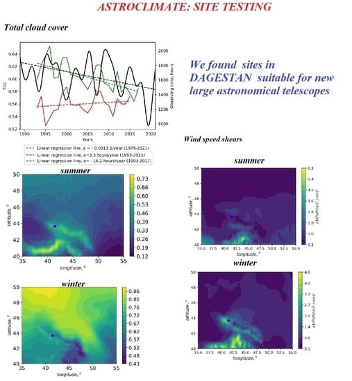
Monthly averaged TCC values were estimated for the BTA site for 1979–2021. Using the Butterworth bandpass filter, changes in the TCC low-frequency component were shown to be in good agreement with the amount of observation time at the telescope. The best time for astronomical observations (in terms of TCC) falls at summer. In particular, for 2002–2021, TCC reaches its minimum in August. The mean TCC is 0.46.

(ii)

The analysis of TCC long-term changes showed that the mean and median values decreased by 0.03 and 0.04, respectively. The duration of astronomical observations has increased by 76 h. The root mean square deviation of TCC remained unchanged. Thus, we believe that the decrease in TCC over a long time interval has led to increased duration of astronomical observations.

(iii)

The analysis of TCC spatial distributions showed that BTA was located between the local TCC maximum with the center to the southwest and the low TCC region extending southeastward in winter. In summer, TCC decreases significantly for the BTA region. However, BTA is located in the region with high TCC (compared to background TCC).

(iv)

The distribution of the $1/$ parameter and vertical integral of kinetic energy within the BTA region indicates that in summer, the quality of astronomical images associated with the lower layers of the atmosphere is higher compared to winter. The higher image quality is due to the greater stability of the free atmosphere (low $1/Ri$), and to BTA location at the periphery of the region with low vertical integral of kinetic energy. The analysis of winter spatial distributions shows that the vast region of low vertical integral of kinetic energy can be associated with the intense process of transformation of the average kinetic energy into the kinetic energy of turbulence. In general, winter is characterized by the increased spatial non-uniformity of vertical movements, presence of pronounced layers in $1/Ri$ vertical profiles, and significant wind speed shears in the lower atmosphere.

(v)

In winter, ERA-5-derived $1/Ri$ in the lower layers of the atmosphere is close to 0.015. This value indicates that turbulence is formed under weak static stability conditions at the BTA site. Stability of the atmosphere increases with height.

(vi)

Using radiosounding data, we estimated the $1/Ri$ integral in the layer from 825 to 650 hPa. The integral is 0.64 in January. The $1/Ri$ decreases in July due to higher repeatability of negative Ri values and amounts to 0.25. In the upper layer of the atmosphere (225–150 hPa), the average $1/Ri$ varies slightly during the year and amounts to 0.25. Overestimated values of $1/Ri$ from radiosounding data in comparison with the reanalysis data are related to insufficient vertical resolution in ERA-5 reanalysis.

(vii)

One of the main conclusions is that potential sites with high astroclimatic parameters are located east and southeast of BTA. Analyzing the spatial distributions of TCC, $1/Ri$, vertical integral of kinetic energy, and the wind speed vertical component, we can conclude that sites suitable for new large astronomical telescopes can be found on the periphery of the low TCC region, in its southeastern part (40.5$°$N–42.0$°$N; 46.2$°$E–48.7$°$E).

(viii)

At the BTA site, the most pronounced atmospheric layer with the wind speed exceeding 15 m/s is observed at the height of ∼12 km [10]. Taking into account the wind speed profiles $V\left(z\right)$ [10] and $1/Ri\left(z\right)$, we can conclude that the conditions for turbulence generation are observed mainly in winter under the jet stream (at 10,300–11,400 m). Under the jet stream, high $1/Ri$ amplitudes and the pattern of changes indicate that turbulence is formed irregularly in this region. Increased strength of fluctuations can be observed only in certain time intervals. These changes allow us to speak about high repeatability of the main parameter of optical turbulence, namely, high values of the Fried parameter $r_0$, estimated for higher atmospheric layers. Compared to the lower atmospheric layers, the repeatability of atmospheric situations with $Ri<0$ at the heights above 200 hPa is insignificant. Using individual $1/Ri\left(z\right)$ profiles, we estimate the repeatability of atmospheric situations with $Ri<0$ for heights above 200 hPa as no more than 10–20% .

(ix)

In winter, high values of wind speed shears are observed in the lower layers of the atmosphere at BTA. In summer, the wind speed vertical shears over BTA are significantly reduced. In the upper troposphere, the situation is the opposite. In winter, BTA is in the region with moderate wind speed shears. In summer, a region with high wind speed shears is formed. Taking into account that $C_n^2$ decreases rapidly with height, better image quality (associated with higher values of the Fried parameter) can be expected in summer. Such energy structure of the atmosphere does not allow applying atmospheric models to describe turbulence based on $C_n\left(z\right)$ as a function of surface values $C_n\left(0\right)$, or to use a model based on turbulence velocity at the height of 200 hPa [35].

The results obtained can be used in the search for new sites suitable for placing new ground-based medium- and large-aperture optical and millimeter telescopes.

References

1. Abbot, H.J.; Munro, J.; Travouillon, T.; Lidman, C.; Tucker, B.E. Archival Weather Conditions at Siding Spring Observatory. Publ. Astron. Soc. Pac. 2021, 133, 95001. [Google Scholar] [CrossRef]
2. Ehgamberdiev, S.A.; Baijumanov, A.K.; Ilyasov, S.P.; Sarazin, M.; Tillayev, Y.A.; Tokovinin, A.A.; Ziad, A. The astroclimate of Maidanak Observatory in Uzbekistan. Astron. Astrophys. Suppl. Ser. 2000, 145, 293–304. [Google Scholar] [CrossRef] [Green Version]
3. Hellemeier, J.A.; Yang, R.; Sarazin, M.; Hickson, P. Weather at selected astronomical sites–an overview of five atmospheric parameters. Mon. Not. R. Astron. Soc. 2019, 482, 4941–4950. [Google Scholar] [CrossRef]
4. Roddier, F. Atmospheric limitations to adaptive image compensation. ASP Conf. Ser. 2002, 266, 546–561. [Google Scholar]
5. Roddier, F. The effects of atmospheric turbulence in optical astronomy. Prog. Opt. 1981, 19, 281–376. [Google Scholar]
6. Kudryavtsev, D.O.; Vlasyuk, V.V. The Largest Russian Optical Telescope BTA: Current Status and Modernization Prospects. In Ground-Based Astronomy in Russia. 21st Century, Proceedings of the All-Russian Conference, Nizhny Arkhyz, Russia, 21–25 September 2020, Special Astrophysical Observatory of the Russian Academy of Sciences; Special Astrophysical Observatory of the Russian Academy of Sciences: Nizhny Arkhyz, Russia, 2020; pp. 21–31. [Google Scholar] [CrossRef]
7. Vlasyuk, V.V. SAO RAS Optical telescopes in the Epoch of multimessenger astronomy. In Ground-Based Astronomy in Russia. 21st Century, Proceedings of the All-Russian Conference, Nizhny Arkhyz, Russia, 21–25 September 2020, Special Astrophysical Observatory of the Russian Academy of Sciences; Special Astrophysical Observatory of the Russian Academy of Sciences: Nizhny Arkhyz, Russia, 2020; pp. 3–11. [Google Scholar] [CrossRef]
8. Khaikin, V.; Lebedev, M.; Shmagin, V.; Zinchenko, I.; Vdovin, V.; Bubnov, G.; Edelman, V.; Yakopov, G.; Shikhovtsev, A.; Marchiori, G.; et al. On the Eurasian SubMillimeter Telescopes Project (ESMT). In Proceedings of the 7th All-Russian Microwave Conference (RMC), Moscow, Russia, 25–27 November 2020; pp. 47–51. [Google Scholar] [CrossRef]
9. Nosov, V.V.; Lukin, V.P.; Nosov, E.V.; Torgaev, A.V.; Afanas’ev, V.L.; Balega, Y.Y.; Vlasyuk, V.V.; Panchuk, V.E.; Yakopov, G.V. Astroclimate Studies in the Special Astrophysical Observatory of the Russian Academy of Sciences. Atmos. Ocean. Opt. 2019, 32, 8–18. [Google Scholar] [CrossRef]
10. Shikhovtsev, A.Y.; Bolbasova, L.A.; Kovadlo, P.G.; Kiselev, A.V. Atmospheric parameters at the 6-m Big Telescope Alt-azimuthal site. Mon. Not. R. Astron. Soc. 2020, 493, 723–729. [Google Scholar] [CrossRef]
11. Han, Y.; Yang, Q.; Liu, N.; Zhang, K.; Qing, C.; Li, X.; Wu, X.; Luo, T. Analysis of wind-speed profiles and optical turbulence above Gaomeigu and the Tibetan Plateau using ERA5 data. Mon. Not. R. Astron. Soc. 2021, 501, 4692–4701. [Google Scholar] [CrossRef]
12. Bounhir, A.; Benkhaldoun, Z.; Carrasco, E.; Sarazin, M. High-altitude wind velocity at Oukaimeden observatory. Mon. Not. R. Astron. Soc. 2009, 398, 862–872. [Google Scholar] [CrossRef] [Green Version]
13. Chueca, S.; García-Lorenzo, B.; Muñoz-Tuñón, C.; Fuensalida, J.J. Statistics and analysis of high-altitude wind above the Canary Islands observatories. Mon. Not. R. Astron. Soc. 2004, 349, 627–631. [Google Scholar] [CrossRef] [Green Version]
14. Qian, X.; Yao, Y.; Wang, H.; Zou, L.; Li, Y. Statistics and analysis of high-altitude wind above the western Tibetan Plateau. Mon. Not. R. Astron. Soc. 2020, 498, 5786–5797. [Google Scholar] [CrossRef]
15. García-Lorenzo, B.; Eff-Darwich, A.; Fuensalida, J.J.; Castro-Almazán, J. Adaptive optics parameters connection to wind speed at the Teide Observatory. Mon. Not. R. Astron. Soc. 2009, 397, 1633–1646. [Google Scholar] [CrossRef] [Green Version]
16. Garcia-Lorenzo, B.; Fuensalida, J.J.; Munoz-Tunon, C.; Mendizabal, E. Astronomical Site Ranking Based on Tropospheric Wind Statistics. Mon. Not. R. Astron. Soc. 2005, 356, 849–858. [Google Scholar] [CrossRef] [Green Version]
17. Hersbach, H.; Bell, B.; Berrisford, P.; Hirahara, S.; Horányi, A.; Muñoz-Sabater, J.; Nicolas, J.; Peubey, C.; Radu, R.; Schepers, D.; et al. The ERA5 global reanalysis. Q. J. R. Meteorol. Soc. 2020, 146, 1999–2049. [Google Scholar] [CrossRef]
18. Virman, M.; Bister, M.; Räisänen, J.; Sinclair, V.A.; Järvinen, H. Radiosonde comparison of ERA5 and ERA-Interim reanalysis datasets over tropical oceans. Tellus A Dyn. Meteorol. Oceanogr. 2021, 73, 1–7. [Google Scholar] [CrossRef]
19. Hach, Y.; Jabiri, A.; Ziad, A.; Bounhir, A.; Sabil, M.; Abahamid, A.; Benkhaldoun, Z. Meteorological profiles and optical turbulence in the free atmosphere with NCEP/NCAR data at Oukaimeden–I. Meteorological parameters analysis and tropospheric wind regimes. Mon. Not. R. Astron. Soc. 2012, 420, 637–650. [Google Scholar] [CrossRef] [Green Version]
20. Cai, J.; Li, X.; Zhan, G.; Wu, P.; Xu, C.; Qing, C.; Wu, X. A new model for the profiles of optical turbulence outer scale and Cn2 on the coast. Acta Phys. Sin. 2018, 67, 014206. [Google Scholar] [CrossRef]
21. Hidalgo, S.L.; Muñoz-Tuñón, C.; Castro-Almazán, J.A.; Varela, A.M. Canarian Observatories Meteorology; Comparison of OT and ORM using Regional Climate Reanalysis. Publ. Astron. Soc. Pac. 2021, 133, 105002. [Google Scholar] [CrossRef]
22. Xu, M.; Shao, S.; Liu, Q.; Sun, G.; Han, Y.; Weng, N. Optical Turbulence Profile Forecasting and Verification in the Offshore Atmospheric Boundary Layer. Appl. Sci. 2021, 11, 8523. [Google Scholar] [CrossRef]
23. Hagelin, S.; Masciadri, E.; Lascaux, F. Optical turbulence simulations at Mt Graham using the Meso-NH model. Mon. Not. R. Astron. Soc. 2011, 412, 2695–2706. [Google Scholar] [CrossRef] [Green Version]
24. Osborn, J.; Sarazin, M. Atmospheric turbulence forecasting with a General Circulation Model for Cerro Paranal. Mon. Not. R. Astron. Soc. 2014, 480, 1278–1299. [Google Scholar] [CrossRef] [Green Version]
25. Panchuk, A.V. Astronomical climate of the telescope installation site and observation time loss. INASAN Sci. Rep. 2020, 5, 344–350. [Google Scholar]
26. Kovadlo, P.G.; Lukin, V.P.; Shikhovtsev, A.Y. Development of the Model of Turbulent Atmosphere at the Large Solar Vacuum Telescope Site as Applied to Image Adaptation. Atmos. Ocean. Opt. 2019, 32, 202–206. [Google Scholar] [CrossRef]
27. Galperin, B.; Sukoriansky, S.; Anderson, P.S. On the critical Richardson number in stably stratified turbulence. Atmos. Sci. Lett. 2007, 8, 65–69. [Google Scholar] [CrossRef]
28. Vinnichenko, N.K.; Pinus, N.Z.; Shmeter, S.M.; Shur, G.N. Turbulence in the Free Atmosphere; Springer: Boston, MA, USA, 1980; Volume 1, 310p. [Google Scholar] [CrossRef]
29. Luce, H.; Hashiguchi, H. On the estimation of vertical air velocity and detection of atmospheric turbulence from the ascent rate of balloon soundings. Atmos. Meas. Tech. 2020, 13, 1989–1999. [Google Scholar] [CrossRef] [Green Version]
30. Lukin, V.P.; Nosov, E.V.; Nosov, V.V.; Torgaev, A.V. Causes of non-Kolmogorov turbulence in the atmosphere. Appl.Opt. 2016, 55, B163–B168. [Google Scholar] [CrossRef]
31. Flores, O.; Riley, J.J. Analysis of Turbulence Collapse in the Stably Stratified Surface Layer Using Direct Numerical Simulation. Bound.-Layer Meteorol. 2011, 139, 241–259. [Google Scholar] [CrossRef]
32. Lotfy, E.R.; Zaki, S.A.; Harun, Z. Modulation of the atmospheric turbulence coherent structures by mesoscale motions. J. Braz. Soc. Mech. Sci. Eng. 2018, 40, 178. [Google Scholar] [CrossRef]
33. Ko, H.-C.; Chun, H.-Y. Potential sources of atmospheric turbulence estimated using the Thorpe method and operational radiosonde data in the United States. Atmos. Res. 2022, 265, 105891. [Google Scholar] [CrossRef]
34. Zhang, J.; Guo, J.; Zhang, S.; Shao, J. Inertia-gravity wave energy and instability drive turbulence: Evidence from a near-global high-resolution radiosonde dataset. Clim. Dyn. 2022, 1–13. [Google Scholar] [CrossRef]
35. Sarazin, M.; Tokovinin, A. The Statistics of Isoplanatic Angle and Adaptive Optics Time Constant derived from DIMM Data. In Beyond Conventional Adaptive Optics, Proceedings of the Topical Meeting, Venice, Italy, 7–10 May 2001; European Southern Observatory: Garching, Germany, 2001; Volume 58, p. 321. [Google Scholar]
Figure 1. Changes in vertical displacements of radiosondes. Lines 1–5 depict the examples of radiosonde runs in January. Lines 6–10 are the examples of radiosonde runs in July. Line 11 shows the averaged profile in January 2021. Line 12 shows the averaged profile in July 2021.
Remotesensing 14 01833 g001
Figure 2. Changes in the monthly averaged values of the total cloud cover at the BTA site for 1979–2021. Red line corresponds to the linear regression line.
Remotesensing 14 01833 g002
Figure 3. Changes in the monthly averaged total cloud cover.
Remotesensing 14 01833 g003
Figure 4. Low-frequency changes in TCC at the BTA site (black line). Amount of observation time at the telescope according to the operation service (green line). Amount of observation time at the telescope according to astronomical observations (red line). Coefficients a characterize line slopes.
Remotesensing 14 01833 g004
Figure 5. High-frequency component of TCC changes.
Remotesensing 14 01833 g005
Figure 6. Energy spectrum of the full TCC time series (orange line) and spectrum of the TCC changes high-frequency component. Black line corresponds to the high-frequency component in TCC changes, and orange line is the spectrum of initial time series.
Remotesensing 14 01833 g006
Figure 7. Distributions of normalized total cloud cover averaged for 2012–2021 within the BTA region (a) in winter and (b) in summer. Blue dot corresponds to BTA location.
Remotesensing 14 01833 g007
Figure 8. Histograms of C n 2 corresponding to the periods (a) from 25 October 2012 to 01 November 2012, and (b) from 30 July 2016 to 7 August 2016.
Remotesensing 14 01833 g008
Figure 9. Spatial distributions of 1 / R i parameter in the 825–650 hPa layer within the BTA region in winter and summer. The distributions are calculated using ERA-5 data for 2012–2021. Blue dot corresponds to BTA location.
Remotesensing 14 01833 g009
Figure 10. Spatial distributions of 1 / R i parameter in the 225–150 hPa layer in winter and summer. The distributions are calculated using ERA-5 data for 2012–2021. Blue dot corresponds to BTA location.
Remotesensing 14 01833 g010
Figure 11. Distributions of wind speed shears in the lower atmospheric layers for 2012–2021 within the BTA region (a) in winter and (b) in summer. Blue dot corresponds to BTA location.
Remotesensing 14 01833 g011
Figure 12. Distributions of wind speed shears in the upper atmospheric layers for 2012–2021 within the BTA region (a) in winter and (b) in summer. Blue dot corresponds to BTA location.
Remotesensing 14 01833 g012
Figure 13. Vertical profiles of 1 / R i at Mineralnye Vody estimated from radiosounding data for January 2021. Red line corresponds to 12 h. Blue line corresponds to 00 h. Black line represents the average profile for two periods.
Remotesensing 14 01833 g013
Figure 14. Vertical profiles of the 1 / R i parameter at the site of Mineralnye Vody, estimated from radiosounding data for July 2021. Red line corresponds to 12 h. Blue line corresponds to 00 h. Black line represents the average profile over two periods.
Remotesensing 14 01833 g014
Figure 15. Vertical integral of kinetic energy for 2012–2021 within the BTA region (a) in winter and (b) in summer. Blue dot corresponds to BTA location.
Remotesensing 14 01833 g015
Figure 16. Wind speed vertical component at 800 hPa pressure level averaged for 2012–2021 within the BTA region (a) in winter and (b) in summer. Blue dot corresponds to BTA location.
Remotesensing 14 01833 g016