
Application of an Improved YOLOv5 Algorithm in Real-Time Detection of Foreign Objects by Ground Penetrating Radar
by
 ,
,
Zhi Qiu
1,2 ,
,
Zuoxi Zhao
1,2,*,
Shaoji Chen
1,2,
Junyuan Zeng
1,2,
Yuan Huang
1,2 and
Borui Xiang
1,2 1
College of Engineering, South China Agricultural University, Guangzhou 510642, China
2
Ministry of Education Key Technologies and Equipment Laboratory of Agricultural Machinery and Equipment in South China, South China Agricultural University, Guangzhou 510642, China
*
Author to whom correspondence should be addressed.
Remote Sens. 2022, 14(8), 1895; https://doi.org/10.3390/rs14081895
Submission received: 17 February 2022
/
Revised: 5 April 2022
/
Accepted: 12 April 2022
/
Published: 14 April 2022
(This article belongs to the Topic Artificial Intelligence in Sensors)
Abstract
:Ground penetrating radar (GPR) detection is a popular technology in civil engineering. Because of its advantages of non-destructive testing (NDT) and high work efficiency, GPR is widely used to detect hard foreign objects in soil. However, the interpretation of GPR images relies heavily on the work experience of researchers, which may lead to problems of low detection efficiency and a high false recognition rate. Therefore, this paper proposes a real-time detection technology of GPR based on deep learning for the application of soil foreign object detection. In this study, the GPR image signal is obtained in real time by the GPR instrument and software, and the image signals are preprocessed to improve the signal-to-noise ratio of the GPR image signals and improve the image quality. Then, in view of the problem that YOLOv5 poorly detects small targets, this study improves the problems of false detection and missed detection in real-time GPR detection by improving the network structure of YOLOv5, adding an attention mechanism, data enhancement, and other means. Finally, by establishing a regression equation for the position information of the ground penetrating radar, the precise localization of the foreign matter in the underground soil is realized.
1. Introduction
Against the background of the current development of unmanned farms, the automation of agricultural machinery is the future trend of agricultural development [1]. Before automatic agricultural production, it is necessary to check underground for hard foreign matter that would be harmful to agricultural machinery and tools, as well as humans and livestock, especially when using the land for the first time; this is a necessary prerequisite for the safe operation of agricultural machinery and tools. Obviously, these hard foreign objects cannot usually be observed by the human eye or cameras [2]. To better understand the characteristics of these foreign objects, researchers have developed an efficient method to detect hard objects buried in soil in real time.
Because electromagnetic wave detection has the advantages of non-destructive detection, a fast detection process, and high detection accuracy, it is widely used for the detection of underground foreign objects [3,4], urban pavement [5,6,7], bridge safety [8,9], and tunnel cavities [10,11], as well as in archaeological exploration [12,13] and other survey experiments. Researchers can use the characteristic components of common GPR two-dimensional cross-sectional images, which specifically appear as images similar to hyperbolic features, allowing researchers to quickly identify whether there is foreign matter in the underground medium [14]. However, raw GPR radar images rarely provide geometric information about buried objects. Moreover, original GPR radar images are often disturbed by noise, such as experimental noise and reflected waves from other materials on the ground surface [15], which is not conducive to researchers determining and interpreting the geometric shape and specific burial location of hard foreign objects. A large portion of GPR images require human assessment by professional researchers [16].
A small amount of GPR data can be well explained by relying on the work experience of researchers, but when a large amount of GPR data is involved, it is very likely to reduce the identification efficiency and is prone to misinterpretation and omission [17]. Therefore, some researchers use deep learning to automatically identify the features of interest in GPR images [18,19]. Algorithms based on a YOLO series neural network framework have good detection speed performance. Yuanhong Li et al. [20] realized a real-time pattern recognition GPR image of YOLOv3 using the TensorFlow framework developed by Google. Compared to YOLOv3 and YOLOv4, YOLOv5 has also made significant progress in small data sets, and the model of YOLOv5 has better robustness and can better distinguish features in GPR images [21].
The main shortcomings of the current GPR instruments include difficulty in synchronizing the process of GPR image data acquisition, GPR image preprocessing, and detection and identification. Although the approximate location of buried foreign objects can be directly determined through GPR images [22,23], it is a very challenging task to determine the location of steel bars and the shape of foreign objects in real time [24]. Therefore, this paper proposes a method to obtain the ground penetrating radar data in real time in the experimental process, preprocess the ground penetrating radar data, and use the improved YOLOv5 network structure to detect and identify foreign objects.
2. Methodology
We used MALA Controller, software developed by the MALA Company, to obtain GPR signal data in real time. On this basis, we filtered GPR data through two-dimensional continuous wavelet changes and gains through the attenuation law of electromagnetic wave amplitude in the underground lossy media so as to improve the SNR of GPR images, and through the improved YOLOv5 network structure to detect and identify the detected foreign object, after the detection of the foreign object at the precise location. In this paper, the GPR real-time detection system based on the improved YOLOv5 network structure is shown in Figure 1.
2.1. Signal Acquisition
We used the MALA GX 750 HDR ground penetrating radar instrument developed by the MALA Company to obtain experimental data, and we used MALA Controller, mobile phone software developed by the MALA Company, to help us understand and interpret the detection results more accurately.
The original signal file of the GPR was saved on the SD card of the mobile phone. We used the Android Debug Bridge (ADB) tool to enhance the Android mobile phone and obtain the GPR file in the SD card folder in real time. This file records a series of A-scan files, which are binary data. We processed the data by removing the spaces, dividing the characters, and rearranging the data according to the content of the protocol to convert it into decimal data, which is convenient for subsequent data processing and imaging technology research.
2.1.1. Time Zero Correction
The ground penetrating radar calculates the burial depth of the target according to the receiving time of the reflected signal, so whether the receiving time of the reflected signal is accurate will determine whether the burial depth is accurate. According to the working principle of the ground penetrating radar, the propagation time of the ground penetrating radar includes the propagation time of the signal in the host, the cable, and the antenna, the coupling propagation time of the signal between the antenna and the ground, and the propagation time of the signal underground. When analyzing the burial depth of foreign objects, we only used the propagation time of the signal in the ground, so we needed to correct the starting point of the radar propagation time.
When the ground penetrating radar is being used for measurement, since the antenna is close to the ground, the positions of the direct wave and the ground reflected wave are relatively close, especially for antennas with a low frequency and long wave. In the entire waveform scanning curve of GPR, the direct wave and the ground reflected wave are combined into one. At this time, the first peak or trough is usually calibrated as time zero to complete more accurate depth positioning, as shown in Figure 2.
2.1.2. Filtering and Gain
The GPR signal obtained through the above operation includes the electromagnetic wave reflected from the foreign object in the underground soil, the underground clutter, and the electromagnetic wave directly reflected through the air and the surface, namely the direct wave and other signals. However, the direct wave had strong energy and large amplitude, and the reflected signal of the shallow target was easily covered by the direct wave, making it difficult to detect the target signal located on the shallow surface, as shown in Figure 3. It was therefore necessary to perform direct wave removal processing on the reflected echo signal.
In this study, two-dimensional continuous wavelet transform was used to remove the direct wave of the ground penetrating radar signal. On the time-space two-dimensional scale, when the spatial scale becomes larger, the two-dimensional continuous wavelet function transform appears flat on the image, as does the direct wave. Therefore, the two-dimensional continuous wavelet transform of the GPR signal can solve the direct wave signal, and then subtract the direct wave signal from the original GPR signal to achieve the effect of filtering the direct wave. Compared to the traditional methods of removing direct waves by means of mean filtering and median filtering, the removal of direct waves by two-dimensional continuous wavelet change will not damage the effective signal. The filtering effect is shown in Figure 4.
Due to the phenomenon of emission and refraction of electromagnetic waves propagating in the soil medium, the reflected echo signal amplitude of the deeply buried target will be small, and it is even difficult to distinguish it in the signal imaging image. Therefore, in a real detection scenario using ground penetrating radar, we needed to amplify the weak echo signal to compensate for the energy attenuation value of the electromagnetic wave propagating in the lossy medium.
In this study, according to Maxwell’s equation, the attenuation law of electromagnetic wave amplitude in the underground lossy medium was deduced, and the gain function was obtained. The amplified echo signal can be obtained by multiplying the gain function as a weight and the reflected echo. The gain function is shown below. The effect of gain processing after the GPR image was filtered is shown in Figure 5.
According to Maxwell’s equations,
The available equation is written as follows:
In the formula, E is the electromagnetic wave intensity, ω is the angular frequency, μ is the magnetic permeability, ε is the permittivity, and σ is the electrical conductivity.
Then, we can obtain the gain function G as follows:
2.2. Improve the YOLOv5 Network Structure
After preprocessing the ground penetrating radar signal and converting it into an image, this study used YOLOv5 for ground penetrating radar target detection. The training flow chart of YOLOv5 in this study is shown in Figure 6:
2.2.1. YOLOv5s Architecture
YOLOv5 is an open-source project that was announced by Ultralytics LLC on GitHub in June 2020. Although it has not published relevant papers, it has been accepted and recognized by many relevant personnel, and its code is still being updated. Compared to YOLOv4, YOLOv5 is built on the PyTorch framework, with simpler support, easier deployment, and fewer model parameters. It also supports conversion to ONNX and CoreML, which is convenient for users to deploy on mobile terminals and embedded devices. It is an engineering version of the YOLO series algorithms and has unmistakable detection performance. Therefore, for the GPR real-time detection in this study, YOLOv5 is more competent than other algorithms of the YOLO series and other series of algorithms.
This study adopted the fifth version of YOLOv5s released by YOLOv5. The basic framework of this version of YOLOv5 can be divided into four parts—Input, Backbone, Neck, and Head. The Input section enriches the dataset through data augmentation. The Backbone part is mainly composed of the Focus, C3, and SPP modules for feature extraction. FPN+PANet is used in the Neck section to aggregate the image features at this stage. The Head section makes target predictions and outputs through the predictions.
The Focus module is used to sample the original image at double intervals in the horizontal and vertical directions. For example, a 640 × 640 RGB three-channel image is directly output to 320 × 320 × 12, which is equivalent to down sampling, and a 3 × 2 convolution layer is performed. This is to reduce the amount of calculation, improve the receptive field without losing feature information, and prepare for subsequent feature extraction.
At first, YOLOv5 did not use the C3 module to extract features but the BottleneckCSP module. The BottleneckCSP module is a combination of the Bottleneck and SCP modules. Bottleneck was proposed by Kaiming He [25]. It first goes through a 1 × 1 convolution kernel, then a 3 × 3 convolution kernel, and then a 1 × 1 convolution kernel, and finally adds the unconvoluted features and the convolutional features. Its role is to improve the depth of the model. The SCP module was proposed by Jianyao Wang [26]. It divides the input into two parts; one part is calculated by a block (such as Bottleneck), and the other part is directly passed through a 1 × 1 convolutional layer, and then joined. The C3 module eliminates a 1 × 1 convolution layer in the BottleneckCSP module and simplifies the network structure to reduce the computational load.
The SPP module [27] is used to first perform a 1 × 1 convolutional layer on the input convolutional layer, then perform three pooling layers of different sizes, and combine the pooling results with the previous 1 × 1 convolutional layer. Finally, the 1 × 1 convolution layer is used to reduce the dimensionality of the joint results. The function of the SPP module is to fuse more features of different resolutions to obtain more information.
Suppose we input a 640 × 640 RGB three-channel image; after passing through the 0th layer Focus module of YOLOv5, a feature map f0 with a size of 320 × 320 and a channel number of 32 is output. The feature map f0 passes through the 3 × 2 convolutional layer of the first layer of YOLOv5 and the C3 module of the second layer and outputs a feature map f1 with a size of 160 × 160 and a channel number of 64. Then, the feature map f1 passes through the 3 × 2 convolutional layer of the third layer of YOLOv5 and the C3 module of the fourth layer and outputs a feature map f2 with a size of 80 × 80 and a channel number of 128. The feature map f2 then passes through the 3 × 2 convolutional layer of the fifth layer of YOLOv5 and the C3 module of the sixth layer and outputs a feature map f3 with a size of 40 × 40 and a channel number of 256. The feature map f3 passes through the 3 × 2 convolutional layer in the seventh layer of YOLOv5, the SPP module in the eighth layer, and the C3 module in the ninth layer, and outputs a feature map f4 with a size of 20 × 20 and a channel number of 512. At this point, YOLOv5 has completed the feature extraction, which is also the entire content of YOLOv5’s Backbone.
Next is the content of YOLOv5’s Neck. The feature map f4 passes through the 1 × 1 convolution layer of the 10th layer of YOLOv5 and outputs a feature map f5 with a size of 20 × 20 and a channel number of 256. Then, the feature map f5 passes through the up sampling layer of the 11th layer of YOLOv5 and outputs a feature map f6 with a size of 40 × 40 and a channel number of 256. Then, the Concat module of the 12th layer of YOLOv5 splices the feature map f6 with the feature map f3 and outputs a feature map f7 with a size of 40 × 40 and a channel number of 512. Similarly, the feature map f7 passes through the C3 module of the 13th layer of YOLOv5 and the 1 × 1 convolutional layer of the 14th layer and outputs a feature map f8 with a size of 40 × 40 and a channel number of 128. The feature map f8 passes through the up sampling layer of the 15th layer and outputs a feature map f9 with a size of 80 × 80 and a channel number of 128.
Then, the Concat module of the 16th layer of YOLOv5 splices the feature map f9 and the feature map f2 and outputs a feature map f10 with a size of 80 × 80 and 256 channels. Then the feature map f10 passes through the C3 module of the 17th layer of YOLOv5 and outputs a feature map f11 with a size of 80 × 80 and a channel number of 128. The feature map f11 passes through the 1 × 1 convolution layer of the 18th layer of YOLOv5 and outputs a feature map f12 with a size of 80 × 80 and a channel number of 18. The feature map f12 will be used for small-scale object detection.
The feature map f11 passes through the 3 × 2 convolutional layer of the 19th layer of YOLOv5, and the output a feature map f13 with a size of 40 × 40 and a channel number of 128. Then, the Concat module of the 20th layer of YOLOv5 splices the feature map f13 and the feature map f8 and outputs a feature map f14 with a size of 40 × 40 and 256 channels. Then, the feature map f14 passes through the C3 module of the 21st layer of YOLOv5 and outputs a feature map f15 with a size of 40 × 40 and a channel number of 256. The feature map f15 passes through the 1 × 1 convolution layer of the 22nd layer of YOLOv5 and outputs a feature map f16 with a size of 40 × 40 and a channel number of 18. The feature map f16 will be used for mesoscale object detection.
The feature map f15 passes through the 3 × 2 convolutional layer of the 23rd layer of YOLOv5 and outputs a feature map f17 with a size of 20 × 20 and a channel number of 256. Then, the Concat module of the 24th layer of YOLOv5 splices the feature map f17 and the feature map f5 and outputs a feature map f18 with a size of 20 × 20 and a channel number of 512. The feature map f18 passes through the C3 module of the 25th layer of YOLOv5 and outputs a feature map f19 with a size of 20 × 20 and a channel number of 512. The feature map f19 passes through the 1 × 1 convolution layer of the 26th layer of YOLOv5 and outputs a feature map f20 with a size of 20 × 20 and a channel number of 18. The feature map f20 will be used for large-scale object detection. The network structure of YOLOv5 is shown in Figure 7.
2.2.2. Improve the YOLOv5s Network Structure
When we actually used YOLOv5 to detect targets in ground penetrating radar images, we found that its detection accuracy was poor, and false and missed detections often occurred, especially for small targets.
In terms of the appeal phenomenon, our guess is that the environment of the underground soil is relatively complex, and there is underground clutter that cannot be filtered. Some underground soil foreign matter targets are displayed in the image closer to this clutter and background, such as some small iron rods, which interfere with the target detection. Therefore, in response to the above problems, we have made some improvements to YOLOv5 to improve its detection performance.
Based on the original YOLOv5, in this study, we replaced the FPN+PANet network with a weighted bidirectional feature pyramid network Bi-FPN, and added the SE attention mechanism. The improved YOLOv5s network structure is shown in Figure 8.
In the convolution process, since large objects have many pixels and small objects have few pixels, the features of the large objects are easily retained, and it is easier to ignore the features of the small objects that are further back. Like YOLOv1, the image is subjected to multiple convolutions and the target is detected with the result of the last convolution. It is difficult to effectively identify targets of different sizes with this method [28,29], as shown in Figure 9a.
YOLOv3 introduces the FPN network structure [30,31] into the original network structure. After multiple convolution down sampling to obtain high semantic information, it is re-up sampled, and the feature layers with the same scale in the up- and down sampling processes are superimposed. Finally, the target is detected by three scale feature layers with different sizes, which ensures the characteristics and information of the target, as shown in Figure 9b.
On the basis of FPN, YOLOv5 uses PANe to aggregate image features [32]. On the basis of FPN’s deep-to-shallow unidirectional fusion, PANet adds secondary fusion from the bottom to the top and uses accurate low-level localization signals to enhance the entire feature hierarchy and promote the flow of information [33], as shown in Figure 10.
However, PANet is only a simple two-way fusion. Since different input features have different resolutions, their contributions to output features are usually unequal. In addition, when PANet performs feature fusion, it only adds different input features directly, which will lead to unbalanced output features, as shown in Figure 11a.
In this study, BiFPN was used to replace the FPN+PANet network [34] of the original YOLOv5, which improved its ability in multi-scale target recognition and the recognition rate of small targets in GPR images without increasing the computational cost [35]. BiFPN uses a fast normalized fusion algorithm, which gives different weights to the features of each layer for fusion so that the network pays more attention to important layers and reduces the node connections of some unnecessary layers. In addition, when the input and output nodes are of the same scale, BiFPN adds an additional input channel to fuse more features without increasing the computational cost, as shown in Figure 11b. The fast normalized fusion algorithm is as follows:
After using BiFPN, the recall rate of YOLOv5 was greatly improved, which meant that the missed detection phenomenon of our ground penetrating radar image target detection was greatly reduced compared to before optimization. For the same image, YOLOv5 could find more targets and improve the detection performance of the target detector. The precision and recall obtained in training with YOLOv5 before and after using the BiFPN network are shown in Figure 12a,b.
In comparing Figure 12a,b it can be seen that after using BiFPN for ground penetrating radar target detection, although the accuracy of YOLOv5 did not change much at nearly 0.8, the recall rate was improved by 0.1, which shows that the performance of ground penetrating radar target detection in BiFPN-YOLOv5 is better compared to FPN+PANet-YOLOv5. This means that compared to before the optimization, the missed detection of our ground penetrating radar image target detection was greatly reduced. For the same image, YOLOv5 can find more targets and improve the detection performance of the target detector.
In addition, we added the SE attention mechanism, which is a channel attention mechanism that was announced by the autonomous driving company Momenta in 2017 [36]; its definition is shown in Figure 13.
The SE attention mechanism divides a bypass branch after the normal convolution operation. First, the Squeeze operation is performed, which compresses the spatial dimension; that is, each two-dimensional feature map becomes a real number, which is equivalent to keeping the number of feature channels unchanged for the pooling operation of the global receptive field. Then there is the Excitation operation, which generates weights for each feature channel via the parameter r, which is learned to explicitly model the correlation between the feature channels. After the weight of each feature channel is obtained, the weight is applied to each original feature channel. Based on a specific task, the importance of different channels can be learned.
After YOLOv5 introduces the SE attention mechanism, the network can automatically learn where each feature channel of the ground penetrating radar image needs attention, that is, on the target. Instead of evenly distributing features across all pixels of the image, it assigns more features to noteworthy points for different task inputs.
In comparing Figure 14a,b, it can be seen that after adding the SE attention mechanism, although the loss function curve had a slower convergence speed, it was more stable, especially the loss function of objection. Before the SE attention mechanism was added, although the obj_loss converged, there were large fluctuations. After adding the mechanism, it was very stable and there were no large fluctuations, which means that our improved YOLOv5 has stronger stability and robustness.
2.2.3. Data Augmentation
YOLOv5 uses many effective data processing methods to increase the accuracy of the training model and reduce the training time, including image perturbation, brightness, contrast, saturation, hue, adding noise, random scaling, random cropping, flip, rotate, random erase, and mosaic data enhancement.
In addition to the above data enhancement algorithm, this study will also enable a hybrid data enhancement method and add the data enhancement method of copy–paste. Copy–paste data augmentation means, just like its name, copying and pasting the target from one sample to another sample so that the richness of the data set can be increased without changing the size of the data set, which improves the robustness and anti-jamming ability of object detection, which is simple but effective [37].
In addition, according to the characteristics of the ground penetrating radar images, the hyperparameters are adjusted accordingly. The hyperparameter settings are shown in Figure 15a,b.
After we turned on the hybrid data enhancement, increased the copy–paste data enhancement method, and adjusted the hyperparameters, we found that the loss function curve was more stable and the value was smaller, which means that our optimized model has stronger robustness and higher accuracy for GPR image target detection. The loss function curves before and after modification are shown in Figure 16a,b.
2.2.4. Improved Prediction Box Regression Loss Function
When using YOLOv5 for target detection, we can easily see that when the IoU threshold was less than or equal to 0.5, the MAP performed well. When it was greater than 0.5, the performance dropped rapidly with the increase in the IoU threshold, which indicates that it is difficult for YOLOv5 to perfectly align the detection box with the target—which is actually a common problem of single-stage target detection algorithms—and the regression accuracy is not enough.
IoU loss is currently the most widely used regression loss algorithm [38], and most detection algorithms use this algorithm. IoU calculates the side length of the intersection of the detection box and the ground-truth box divided by the side length of the union. The definitions of IoU and IoU loss are as follows:
where represents the ground-truth box and represents the predicted box.
However, IoU loss cannot optimize the situation where the prediction box and the target box do not intersect, and IoU = 0. When two boxes intersect, the IoU value cannot reflect where the two boxes intersect.
GIoU is proposed to overcome the shortcomings of IoU and make full use of its advantages [39]. GIoU adds a penalty function of the overlapping area scale between the detection box and the ground-truth box [40], which is defined as follows:
where C represents a box that can contain both the predicted box and the ground-truth box.
Compared to IoU, GIoU can completely avoid the problem of the detection frame and the real frame not intersecting, when the gradient will be 0, which cannot be optimized. Secondly, it can also distinguish the alignment of the box. The regression loss function of the prediction box of YOLOv5 adopts GIoU. However, GIoU also has its shortcomings. When the detection frame has an inclusive relationship with the real frame, GIoU will degenerate into IoU, which cannot reflect the intersection position. Moreover, GIoU relies too much on IoU, and its convergence rate is slow.
In order to overcome the problems of the slow convergence of GIoU and the insufficient accuracy of the detection box regression, this study adopted CIoU. CIoU adds a penalty function for the scale of the overlapping area, center point distance, and aspect ratio [41]. CIoU is defined as follows:
where represent the width and height of , respectively, and represent the width and height of B, respectively.
Compared to GIoU, in the actual training iteration process of CIoU, the center point distance between the detection box and the prediction box is closer, the overlapping area is bigger, and the convergence speed is faster, which indicates that CIoU’s regression loss function has better predictive performance.
In comparing Figure 17a,b, it can be seen that when using the CIoU function, the loss function curve converged faster and was more stable, which means that CIoU has stronger robustness and higher accuracy, and fewer iterations are required to train the same model.
It can be seen in Table 1 that after using the CIoU loss function, the mAP obtained by YOLOv5 for different IoU non-maximum suppression in GPR target detection was larger than that of GIoU, which shows that under different IoU NMS, CIoU-YOLOv5 has better regression accuracy. That is to say, in the detection of ground penetrating radar targets, it has higher positioning accuracy, which lays the foundation for us to accurately locate foreign objects in underground soil.
2.2.5. Ablation Experiment
For the above improvements, we did ablation experiments to compare the effects before and after the improvements. The dataset used in this study includes 483 GPR images with a total of 2124 labels. We divided these labels into a training set, validation set, and test set at a ratio of 7:2:1 and trained and tested them on a server with a Tesla V100 graphics card. The number of iterations was 300 epochs.
Here, we chose the average precision (AP), which is defined as follows:
where TP is the number of correctly detected targets, FP is the number of non-targets that the detector considers to be targets, and FN is the number of non-targets that the detector considers.
It can be seen in Table 2 that after the improvement, the recall rate was greatly improved compared to that before the improvement. Specifically, it was improved by 0.18, and the average accuracy was also improved by nearly 0.15, which means that our improved detector will better reduce the phenomenon of missed detection and false detection in the GPR image target detection task.
2.3. Ground Penetrating Radar Target Precise Positioning
After the target detection of the underground hard foreign matter in the soil, we needed to excavate it, so we needed to know the real-world coordinates and buried depth of where the target was detected. However, according to the GPR signal storage file, the abscissa of the coordinate axis of the GPR signal on the image only had the relative displacement from the starting point, and displayed all the targets on the path, that is, when we use the improved YOLOv5 to detect the targets in the GPR image, we can only obtain the pixel coordinates of all foreign objects on the path. This cannot meet the needs of a real application. Through the conversion of world coordinates, we judged whether there was a foreign object directly below, and obtained the position of the GPR GPS. When YOLOv5 detects a foreign object directly below, the system immediately records the buried depth of the foreign object and the GPS position.
2.3.1. Obtaining a GPS Signal
We used the ADB tool to enhance Android phones and obtain the ground penetrating radar CorTmp file in the SD card folder in real time. The file records the date, time, latitude and longitude, mode, and thread of the ground penetrating radar at that time. We preprocessed the data, deleted spaces, split characters, and obtained the latitude and longitude information.
2.3.2. Determining Whether There Is a Foreign Object Directly Below
When YOLOv5 detects a foreign object in the ground penetrating radar image, it will generate a prediction box (the coordinates of the upper left corner, the coordinates of the lower right corner). We needed to find the vertices of the foreign object image according to the prediction box, that is, the vertices of the hyperbola, and then compare the coordinates of all hyperbolic vertices and find the one with the largest pixel coordinates. Then the same method was used to detect the next frame of the image to obtain the largest hyperbolic vertex in the pixel coordinates of the next frame of the image. If the distance in the pixel coordinates of the hyperbolic vertex coordinates at this time was larger than that of the previous frame, it meant that there was a foreign object below. To sum up, the flowchart of this study for judging whether there is a foreign object directly below is shown in Figure 18.
However, because the signal receiving end of the ground penetrating radar has a delay, that is to say, when the ground penetrating radar image detects a foreign object directly under the above operation, it has actually passed the foreign object, so we needed to compensate for it. At first, we wanted to establish a ternary regression equation (x, y, t) from the starting point to the latitude and longitude of this frame. According to the delay time at the receiving end of the GPR, we calculated the longitude and latitude of crossing foreign objects and conducted the compensation. However, it failed because the longitude and latitude are two independent variables. Therefore, we decided to establish a regression equation between the longitude and dimension and time alone.
Because the ground penetrating radar adopts a time-triggered method, in the real survey, we fixed the ground penetrating radar onto an all-terrain vehicle, and then let the all-terrain vehicle drive at a constant speed. The all-terrain vehicle was in a state of acceleration for a period of time when it started and was in a state of constant speed behind, so we needed to iterate the regression equation. However, the amount of data was too large after driving for a period of time. If it continues to iterate, it requires a large amount of calculation. At the same time, because the delay distance of the ground penetrating radar signal receiving end was relatively short compared to the distance the vehicle traveled, this study adopted the method of reading the last 50 frames of the GPS coordinates used to establish the regression equation. In this way, the moving equation of the current speed of the all-terrain vehicle could be approximated, and the amount of calculation was reduced.
2.3.3. World Coordinate Transformation
The ordinate of the pixel coordinates of the ground penetrating radar image corresponds to the depth of the ground penetrating radar signal in the soil. In order to know the specific buried depth of the foreign object, it was necessary to convert the pixel coordinates into world coordinates. Here, we could easily find that the pixel coordinates of the image had a proportional relationship with the real-world coordinates, so we took the direct wave of the ground penetrating radar image as the starting point of the world coordinates, and did experiments to determine them, including burying a foreign object at 50 cm and determining its position in the image pixel coordinates to establish its corresponding relationship. Assuming that the pixel coordinate of the foreign object in the image is z, and the world coordinate is Z, then its proportional relationship is as follows:
Then, the real depth of the foreign object is as follows:
Of course, there are errors in this method. For this reason, we performed multiple sets of experiments and averaged the proportional coefficients obtained from these experiments to reduce errors.
2.4. Ground Penetrating Radar Experiment
The experiment of this study was completed in the Key Laboratory of Key Technology of Agricultural Machinery and Equipment in the Southern Ministry of Education. In the experiment, a common farmland soil platform in southern China was built. The dimensions of the soil platform were 6 m in length, 2 m in width, and 1.5 m in depth, and it included a batch of iron experimental materials, such as steel bars, iron plate materials, and so forth, as shown in Figure 19a. The detection experiment in this study adopted the high dynamic ground penetrating radar MALA GX 750 HDR instrument developed by the MALA Company. It collected 412 samples in each channel with a sampling spacing of 0.015 m. The coupling spacing of the GPR antenna was 0.14 m, and the diameter of the ranging wheel of the GPR instrument was 17 cm. At the same time, we used MALA Controller, a software developed by the MALA Company, to help us understand and interpret the detection results more intuitively. The real-time detection system of the GPR instrument built is shown in Figure 19b.
Since sand is a non-transparent material, the sand on the experimental platform needed to be leveled before the experiment was carried out, which not only provided a reliable guarantee for the accuracy of the buried depth of the steel bars in our later measurement but also ensured the measurement accuracy of the distance measuring wheel. After the sand surface was leveled, the steel bars were buried in the sand according to the pre-designed experimental plan. At this time, we recorded the burial depth as the distance between the steel bars and the sand surface. After burying the rebars at a known distance, we filled the sand surface to the same level as before burying the rebars.
It is worth noting that, before the experiment started, we chose to set the propagation speed of the electromagnetic waves in different media according to our research experience. However, in real soil, there are many factors that interfere with the propagation speed of electromagnetic waves in the medium. Therefore, we also performed a pre-experiment, in which we used the Hyperbola fitting function of MALA Controller to fit the hyperbola feature in the GPR image based on the GPR image obtained in the MALA Controller software, which more accurately obtained the propagation speed of the electromagnetic waves in the current detection medium, which also ensured good detection accuracy for the real-time detection experiments. As shown in Figure 20, the propagation velocity of the electromagnetic waves in this medium was quickly obtained at the scene by fitting with the hyperbolic curve of the measured object, which was 184 (m/μs).
However, the images in the mobile phone MALA Controller software did not undergo preprocessing methods, such as filtering and enhancement of the original signal, and their signal-to-noise ratio was poor, often masking the target signal. Moreover, the recognition of the ground penetrating radar image on the mobile phone screen was affected by the pixels of the mobile phone, which led to poor image quality. Fortunately, MALA Controller saved the original signal file during the experiment, so we processed the original signal. The real-time detection results of ground penetrating radar based on the improved YOLOv5 network structure are shown in Figure 21 and Figure 22.
3. Results and Discussion
3.1. Detection Effect
We used YOLOv5 in Section 2.2 and our improved YOLOv5 to analyze ground penetrating radar images, and compared their detection of the subsurface soil foreign objects under a single category of effects, including the correct recognition rate, missed detection rate, and false detection rate. Below is a comparison between our detector and YOLOv5 in a real detection scenario.
In Figure 23, there are seven foreign object targets in the ground penetrating radar image, including two small targets and a hyperbolic overlapping target. Regarding missed detection, it can be seen that YOLOv5 only detected five foreign object targets, and missed a small target and an overlapping target, but our improved target detector detected all seven foreign object targets. Both the YOLOv5 algorithm and our improved detector had no false detections.
In Figure 24, there are eight foreign object targets in the ground penetrating radar image. Regarding missed detection, the YOLOv5 algorithm and our improved target detector detected all eight foreign object targets. Both the YOLOv5 algorithm and our improved detector had no false detections.
In Figure 25, there are eight foreign object targets in the ground penetrating radar image. Regarding missed detection, it can be seen that the YOLOv5 algorithm only detected six foreign object targets and missed a small target and a target with an overlapping phenomenon, but our improved target detector detected all eight foreign object targets. However, regarding false detection, our improved detector falsely detected two targets. This may be because, from the perspective of the local view, the part boxed out by our improved detector had similar characteristics to the hyperbolic feature, and there may have been here. However, in this experiment, we did not train samples on the void phenomenon, which shows that our improved detector has a stronger generalization ability and robustness.
In Figure 26, there are several small foreign object targets and two large foreign object targets in the ground penetrating radar image. Regarding missed detection, it can be seen that the YOLOv5 algorithm only detected one large foreign object target and missed another large target. However, our improved target detector detected all of the foreign objects. Regarding the false detection phenomenon, our improved detector detected a false target. We assumed that the small target boxed out by the improved detector may have been a foreign object that we ignored in the beginning, such as an iron rod small in diameter. This shows that our improved detector has a stronger generalization ability and robustness.
In comparing these four sets of graphs, on the whole, our improved detector had higher confidence and regression accuracy than the YOLOv5 algorithm, and the predicted box of the improved detector had a higher degree of coincidence with our expected real box. In the subsequent processing, we needed to use the prediction box of the detector for depth positioning, and the excellent regression accuracy provided certain conditions for us to accurately locate foreign objects in the underground soil.
3.2. Model Comparison
In addition, we compared other excellent target detectors, such as fast RCNN and SSD, under the same training scenario to verify that the improved YOLOv5 we used is more suitable for real-time detection of our ground penetrating radar.
3.2.1. Model Evaluation Metrics
In this study, we selected some commonly used metrics to evaluate the model, including precision (P), recall (R), average precision (AP), F1 score, inference time, and model size. These metrics are defined as follows:
where TP is the number of correctly detected targets, FP is the number of non-targets that the detector considers to be targets, and FN is the number of non-targets that the detector considers.
3.2.2. Detector Comparison
We used the same data set in this study to compare the performance of the better two-stage and single-stage target detection algorithms at the current stage, such as fast RCNN and SSD, with our improved YOLOv5 algorithm. The comparison results are shown in Table 3.
Compared to the original YOLOv5, although the memory space occupied by the improved YOLOv5 model is a little larger, all aspects of performance indicators have been greatly improved, and compared to fast RCNN and SSD, the increase in the memory space of the model can be ignored. In comparing the improved YOLOv5 model to fast RCNN, the recall rate is lower, but it has higher accuracy and detection speed. Compared to the SSD, although it is inferior in accuracy and detection speed, the recall rate and average accuracy are far superior. Overall, the detection speed of our improved YOLOv5 meets the standard of real-time detection and has more balanced recall and accuracy compared to fast RCNN and SSD, which means that it has better detection performance in the target detection task of a GPR image. It can reduce the phenomenon of false detection and missed detection, and is more suitable for the needs of real-time detection of GPR image targets.
4. Conclusions
In this study, through the preprocessing of the original signal of ground penetrating radar, the improved YOLOv5 was used for target detection, the target was accurately positioned after the detection, and the real-time detection and positioning of the ground penetrating radar were realized. The contributions of this paper are as follows:
- (1)
- We improved the network structure of YOLOv5, used BiFPN instead of FPN+PANet, added a smaller target detection layer, used the CIoU loss function instead of the GIoU loss function, and added copy–paste data enhancement methods to the data enhancement, which had better accuracy and robustness than without the improvement, and reduced the false detection and missed detection rate.
- (2)
- After we detected the target, we used the regression equation and the supervision function to compensate for the inaccurate positioning caused by the signal delay of the ground penetrating radar receiver, and realized that when a foreign object in the underground soil is detected, the global longitude, latitude, and burial depth of the foreign object can be known in real time, which is convenient for the subsequent processing of an unmanned farm.
- (3)
- We solved the problem of unsatisfactory GPR image quality obtained by taking screenshots with MALA’s mobile phone software, which are easily affected by the screen resolution of the mobile phone. After we obtained the ground penetrating radar image signal, we filtered out the interference of the direct wave and enhanced the filtered signal so as to obtain a better ground penetrating radar image, which is convenient for subsequent target detection.
Author Contributions
Conceptualization, Z.Z. and Z.Q.; methodology, Z.Q.; software, J.Z.; validation, Y.H.; formal analysis, S.C.; investigation, B.X.; data curation, Y.H.; writing—original draft preparation, Z.Q.; writing—review and editing, J.Z. and Y.H.; funding acquisition, Z.Z. All authors have read and agreed to the published version of the manuscript.
Funding
The authors would like to acknowledge the support of this study by the Guangdong Provincial Department of Agriculture’s Modern Agricultural Innovation Team Program for Animal Husbandry Robotics (Grant No. 2019KJ129), the State Key Research Program of China (Grant No. 2016YFD0700101), the Vehicle Soil Parameter Collection and Testing Project (Grant No. 4500-F21445), and the Special project of Guangdong Provincial Rural Revitalization Strategy in 2020 (YCN [2020] No. 39) (Fund No. 200-2018-XMZC-0001-107-0130).
Institutional Review Board Statement
Not applicable.
Informed Consent Statement
Not applicable.
Conflicts of Interest
The authors declare no conflict of interest.
References
- Wang, T.; Xu, X.; Wang, C.; Li, Z.; Li, D. From Smart Farming towards Unmanned Farms: A New Mode of Agricultural Production. Agriculture 2021, 11, 145. [Google Scholar] [CrossRef]
- Zang, G.; Sun, L.; Chen, Z.; Li, L. A nondestructive evaluation method for semi-rigid base cracking condition of asphalt pavement. Constr. Build. Mater. 2018, 162, 892–897. [Google Scholar] [CrossRef]
- Li, Y.; Zhao, Z.; Xu, W.; Liu, Z.; Wang, X. An effective FDTD model for GPR to detect the material of hard objects buried in tillage soil layer. Soil Tillage Res. 2019, 195, 104353. [Google Scholar] [CrossRef]
- Meschino, S.; Pajewski, L.; Pastorino, M.; Randazzo, A.; Schettini, G. Detection of subsurface metallic utilities by means of a SAP technique: Comparing MUSIC- and SVM-based approaches. J. Appl. Geophys. 2013, 97, 60–68. [Google Scholar] [CrossRef]
- Kim, N.; Kim, K.; An, Y.; Lee, H.; Lee, J. Deep learning-based underground object detection for urban road pavement. Int. J. Pavement Eng. 2020, 21, 1638–1650. [Google Scholar] [CrossRef]
- Hong, W.; Kang, S.; Lee, S.J.; Lee, J. Analyses of GPR signals for characterization of ground conditions in urban areas. J. Appl. Geophys. 2018, 152, 65–76. [Google Scholar] [CrossRef]
- Krysiński, L.; Sudyka, J. GPR abilities in investigation of the pavement transversal cracks. J. Appl. Geophys. 2013, 97, 27–36. [Google Scholar] [CrossRef]
- Abouhamad, M.; Dawood, T.; Jabri, A.; Alsharqawi, M.; Zayed, T. Corrosiveness mapping of bridge decks using image-based analysis of GPR data. Autom. Constr. 2017, 80, 104–117. [Google Scholar] [CrossRef]
- Solla, M.; Lorenzo, H.; Novo, A.; Caamaño, J.C. Structural analysis of the Roman Bibei bridge (Spain) based on GPR data and numerical modelling. Autom. Constr. 2012, 22, 334–339. [Google Scholar] [CrossRef]
- Wei, L.; Magee, D.R.; Cohn, A.G. An anomalous event detection and tracking method for a tunnel look-ahead ground prediction system. Automat. Constr. 2018, 91, 216–225. [Google Scholar] [CrossRef] [Green Version]
- Feng, D.; Wang, X.; Zhang, B. Specific evaluation of tunnel lining multi-defects by all-refined GPR simulation method using hybrid algorithm of FETD and FDTD. Constr. Build. Mater. 2018, 185, 220–229. [Google Scholar] [CrossRef]
- Cuenca-García, C.; Risbøl, O.; Bates, C.R.; Stamnes, A.A.; Skoglund, F.; Ødegård, Ø.; Viberg, A.; Koivisto, S.; Fuglsang, M.; Gabler, M.; et al. Sensing Archaeology in the North: The Use of Non-Destructive Geophysical and Remote Sensing Methods in Archaeology in Scandinavian and North Atlantic Territories. Remote Sens. 2020, 12, 3102. [Google Scholar] [CrossRef]
- Papadopoulos, N.; Sarris, A.; Yi, M.; Kim, J. Urban archaeological investigations using surface 3D Ground Penetrating Radar and Electrical Resistivity Tomography methods. Explor. Geophys. 2018, 40, 56–68. [Google Scholar] [CrossRef]
- Ramya, M.; Balasubramaniam, K.; Shunmugam, M.S. On a reliable assessment of the location and size of rebar in concrete structures from radargrams of ground-penetrating radar. Insight Non-Destr. Test. Cond. Monit. 2016, 58, 264–270. [Google Scholar] [CrossRef]
- Li, W.; Cui, X.; Guo, L.; Chen, J.; Chen, X.; Cao, X. Tree Root Automatic Recognition in Ground Penetrating Radar Profiles Based on Randomized Hough Transform. Remote Sens. Basel 2016, 8, 430. [Google Scholar] [CrossRef] [Green Version]
- Jin, Y.; Duan, Y. Wavelet Scattering Network-Based Machine Learning for Ground Penetrating Radar Imaging: Application in Pipeline Identification. Remote Sens. 2020, 12, 3655. [Google Scholar] [CrossRef]
- Jiao, L.; Ye, Q.; Cao, X.; Huston, D.; Xia, T. Identifying concrete structure defects in GPR image. Measurement 2020, 160, 107839. [Google Scholar] [CrossRef]
- Qin, H.; Zhang, D.; Tang, Y.; Wang, Y. Automatic recognition of tunnel lining elements from GPR images using deep convolutional networks with data augmentation. Automat. Constr. 2021, 130, 103830. [Google Scholar] [CrossRef]
- Dinh, K.; Gucunski, N.; Duong, T.H. An algorithm for automatic localization and detection of rebars from GPR data of concrete bridge decks. Automat. Constr. 2018, 89, 292–298. [Google Scholar] [CrossRef]
- Li, Y.; Zhao, Z.; Luo, Y.; Qiu, Z. Real-Time Pattern-Recognition of GPR Images with YOLO v3 Implemented by Tensorflow. Sensors 2020, 20, 6476. [Google Scholar] [CrossRef]
- Li, S.; Gu, X.; Xu, X.; Xu, D.; Zhang, T.; Liu, Z.; Dong, Q. Detection of concealed cracks from ground penetrating radar images based on deep learning algorithm. Constr. Build. Mater. 2021, 273, 121949. [Google Scholar] [CrossRef]
- Agred, K.; Klysz, G.; Balayssac, J.P. Location of reinforcement and moisture assessment in reinforced concrete with a double receiver GPR antenna. Constr. Build. Mater. 2018, 188, 1119–1127. [Google Scholar] [CrossRef]
- Maas, C.; Schmalzl, J. Using pattern recognition to automatically localize reflection hyperbolas in data from ground penetrating radar. Comput. Geosci. UK 2013, 58, 116–125. [Google Scholar] [CrossRef]
- Feng, D.; Wang, X.; Wang, X.; Ding, S.; Zhang, H. Deep Convolutional Denoising Autoencoders with Network Structure Optimization for the High-Fidelity Attenuation of Random GPR Noise. Remote Sens. 2021, 13, 1761. [Google Scholar] [CrossRef]
- Mao, S.; Rajan, D.; Chia, L.T. Deep residual pooling network for texture recognition. Pattern Recogn. 2021, 112, 107817. [Google Scholar] [CrossRef]
- Wang, C.Y.; Liao, H.Y.M.; Wu, Y.H.; Chen, P.Y.; Hsieh, J.W.; Yeh, I.H. CSPNet: A new backbone that can enhance learning capability of CNN. In Proceedings of the IEEE/CVF Conference on Computer Vision and Pattern Recognition Workshops, Seattle, WA, USA, 14–19 June 2020; pp. 390–391. [Google Scholar]
- He, K.; Zhang, X.; Ren, S.; Sun, J. Spatial Pyramid Pooling in Deep Convolutional Networks for Visual Recognition. IEEE Trans. Pattern Anal. Mach. Intell. 2015, 37, 1904–1916. [Google Scholar] [CrossRef] [Green Version]
- Hu, J.; Shi, C.J.R.; Zhang, J. Saliency-based YOLO for single target detection. Knowl. Inf. Syst. 2021, 63, 717–732. [Google Scholar] [CrossRef]
- Redmon, J.; Divvala, S.; Girshick, R.; Farhadi, A. You only look once: Unified, real-time object detection. In Proceedings of the IEEE Conference on Computer Vision and PATTERN recognition, Las Vegas, NV, USA, 27–30 June 2016; pp. 779–788. [Google Scholar]
- Redmon, J.; Farhadi, A. YOLOv3: An Incremental Improvement. arXiv 2018, arXiv:1804.02767. [Google Scholar]
- Lin, T.Y.; Dollár, P.; Girshick, R.; He, K.; Hariharan, B.; Belongie, S. Feature pyramid networks for object detection. In Proceedings of the IEEE Conference on Computer Vision and Pattern Recognition, Honolulu, HI, USA, 21–26 July 2017; pp. 2117–2125. [Google Scholar]
- Liu, S.; Qi, L.; Qin, H.; Shi, J.; Jia, J. Path Aggregation Network for Instance Segmentation. In Proceedings of the IEEE Conference on Computer Vision and Pattern Recognition, Salt Lake City, UT, USA, 18–23 June 2018; pp. 8759–8768. [Google Scholar]
- Yan, B.; Fan, P.; Lei, X.; Liu, Z.; Yang, F. A Real-Time Apple Targets Detection Method for Picking Robot Based on Improved YOLOv5. Remote Sens. 2021, 13, 1619. [Google Scholar] [CrossRef]
- Tan, M.; Pang, R.; Le, Q.V. EfficientDet: Scalable and Efficient Object Detection. In Proceedings of the IEEE/CVF Conference on Computer Vision and Pattern Recognition, Seattle, WA, USA, 13–19 June 2020; pp. 10781–10790. [Google Scholar]
- Rios-Cabrera, R.; Lopez-Juarez, I.; Maldonado-Ramirez, A.; Alvarez-Hernandez, A.; Maldonado-Ramirez, A.D.J. Dynamic categorization of 3D objects for mobile service robots. Ind. Robot. Int. J. Robot. Res. Appl. 2020, 48, 51–61. [Google Scholar] [CrossRef]
- Hu, J.; Shen, L.; Sun, G. Squeeze-and-excitation networks. In Proceedings of the IEEE Conference on Computer Vision and Pattern Recognition, Salt Lake City, UT, USA, 18–23 June 2018; pp. 7132–7141. [Google Scholar]
- Ghiasi, G.; Cui, Y.; Srinivas, A.; Qian, R.; Lin, T.Y.; Cubuk, E.D.; Le, Q.V.; Zoph, B. Simple copy-paste is a strong data augmentation method for instance segmentation. In Proceedings of the IEEE/CVF Conference on Computer Vision and Pattern Recognition, Nashville, TN, USA, 20–25 June 2021; pp. 2918–2928. [Google Scholar]
- Yu, J.; Jiang, Y.; Wang, Z.; Cao, Z.; Huang, T. UnitBox: An Advanced Object Detection Network. In Proceedings of the 24th ACM international conference on Multimedia, New York, NY, USA, 15–19 October 2016; pp. 516–520. [Google Scholar]
- Rezatofighi, H.; Tsoi, N.; Gwak, J.; Sadeghian, A.; Reid, I.; Savarese, S. Generalized Intersection over Union: A Metric and A Loss for Bounding Box Regression. In Proceedings of the IEEE/CVF Conference on Computer Vision and Pattern Recognition, Long Beach, CA, USA, 15–20 June 2019; pp. 658–666. [Google Scholar]
- Zhang, H.; An, L.; Chu, V.W.; Stow, D.A.; Liu, X.; Ding, Q. Learning Adjustable Reduced Downsampling Network for Small Object Detection in Urban Environments. Remote Sens. 2021, 13, 3608. [Google Scholar] [CrossRef]
- Zheng, Z.; Wang, P.; Ren, D.; Liu, W.; Ye, R.; Hu, Q.; Zuo, W. Enhancing Geometric Factors in Model Learning and Inference for Object Detection and Instance Segmentation. IEEE Trans. Cybern. 2021. [Google Scholar] [CrossRef] [PubMed]
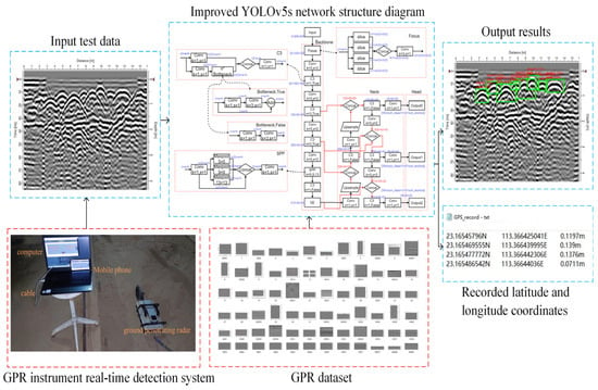
Figure 1.
Schematic diagram of the real-time detection system of ground penetrating radar based on the improved YOLOv5 network structure.
Figure 1.
Schematic diagram of the real-time detection system of ground penetrating radar based on the improved YOLOv5 network structure.

Figure 2.
Schematic diagram of time zero calibration.

Figure 3.
Ground penetrating radar image with direct wave front removed.

Figure 4.
Ground penetrating radar image after removing the direct wave.

Figure 5.
GPR image after gain.

Figure 6.
Training flow chart of YOLOv5.

Figure 7.
YOLOv5s network structure diagram.

Figure 8.
Improved YOLOv5s network structure diagram.

Figure 9.
(a) Single feature layer structure; (b) FPN structure.

Figure 10.
FPN+PANet structure.

Figure 11.
(a) Schematic diagram of PANet network; (b) schematic diagram of BiFPN network.

Figure 12.
(a) Precision and recall plot of FPN+PANet; (b) precision and recall plot of BiFPN.

Figure 13.
Schematic diagram of SE adding attention mechanism.

Figure 14.
(a) SE attention mechanism not added; (b) adding SE attention mechanism.

Figure 15.
(a) Super parameters before modification; (b) modified hyperparameters.

Figure 16.
(a) Loss function before modification; (b) loss function after modification.

Figure 17.
(a) GIoU decline curve during training; (b) CIoU loss decline curve during training.

Figure 18.
Flow chart for judging whether there is a foreign object directly below.

Figure 19.
(a) Iron experimental material; (b) GPR instrument real-time detection system.

Figure 20.
Quickly obtained propagation speed of electromagnetic waves in this medium.

Figure 21.
Target location results of ground penetrating radar image 1.

Figure 22.
Target location results of ground penetrating radar image 2.

Figure 23.
(a) Original image; (b) foreign objects expected to be detected; (c) foreign objects detected by the YOLOv5 algorithm; (d) foreign objects detected by the improved YOLOv5 algorithm.
Figure 23.
(a) Original image; (b) foreign objects expected to be detected; (c) foreign objects detected by the YOLOv5 algorithm; (d) foreign objects detected by the improved YOLOv5 algorithm.

Figure 24.
(a) Original image; (b) foreign objects expected to be detected; (c) foreign objects detected by the YOLOv5 algorithm; (d) foreign objects detected by the improved YOLOv5 algorithm.
Figure 24.
(a) Original image; (b) foreign objects expected to be detected; (c) foreign objects detected by the YOLOv5 algorithm; (d) foreign objects detected by the improved YOLOv5 algorithm.


Figure 25.
(a) Original image; (b) foreign objects expected to be detected; (c) foreign objects detected by the YOLOv5 algorithm; (d) foreign objects detected by the improved YOLOv5 algorithm.
Figure 25.
(a) Original image; (b) foreign objects expected to be detected; (c) foreign objects detected by the YOLOv5 algorithm; (d) foreign objects detected by the improved YOLOv5 algorithm.

Figure 26.
(a) Original image; (b) foreign objects expected to be detected; (c) foreign objects detected by the YOLOv5 algorithm; (d) foreign objects detected by the improved YOLOv5 algorithm.
Figure 26.
(a) Original image; (b) foreign objects expected to be detected; (c) foreign objects detected by the YOLOv5 algorithm; (d) foreign objects detected by the improved YOLOv5 algorithm.


Table 1.
mAP values of GIoU-YOLOv5 and CIoU-YOLOv5 under different IoU NMS.
| IoU0.5 | IoU0.6 | IoU0.7 | IoU0.8 | IoU0.9 | IoU0.95 | |
|---|---|---|---|---|---|---|
| GIoU | 0.609 | 0.598 | 0.567 | 0.484 | 0.311 | 0.227 |
| CIoU | 0.653 | 0.643 | 0.616 | 0.546 | 0.382 | 0.264 |
Table 2.
Performance comparison before and after using different improvements.
| None | BiFPN | SE | Data Augmentation | CIoU | P | R | mAP |
|---|---|---|---|---|---|---|---|
| √ | 0.860 | 0.494 | 0.610 | ||||
| √ | √ | 0.757 | 0.682 | 0.732 | |||
| √ | 0.783 | 0.542 | 0.609 | ||||
| √ | √ | 0.776 | 0.599 | 0.653 | |||
| √ | √ | √ | √ | 0.826 | 0.680 | 0.757 |
Table 3.
Performance comparison of detection algorithms.
| Fast RCNN | SSD | YOLOv5 | Ours | |
|---|---|---|---|---|
| P | 0.558 | 0.905 | 0.86 | 0.826 |
| R | 76.2 | 0.473 | 0.496 | 0.68 |
| AP | 0.731 | 0.656 | 0.63 | 0.757 |
| F1 | 0.64 | 0.62 | 0.68 | 0.73 |
| Inference time | 56.2 ms | 8.14 ms | 9.5 ms | 9.1 ms |
| Weight | 108 MB | 90.6 MB | 13.6 MB | 16.1 MB |
Publisher’s Note: MDPI stays neutral with regard to jurisdictional claims in published maps and institutional affiliations. |
© 2022 by the authors. Licensee MDPI, Basel, Switzerland. This article is an open access article distributed under the terms and conditions of the Creative Commons Attribution (CC BY) license (https://creativecommons.org/licenses/by/4.0/).
Share and Cite
MDPI and ACS Style
Qiu, Z.; Zhao, Z.; Chen, S.; Zeng, J.; Huang, Y.; Xiang, B. Application of an Improved YOLOv5 Algorithm in Real-Time Detection of Foreign Objects by Ground Penetrating Radar. Remote Sens. 2022, 14, 1895. https://doi.org/10.3390/rs14081895
AMA Style
Qiu Z, Zhao Z, Chen S, Zeng J, Huang Y, Xiang B. Application of an Improved YOLOv5 Algorithm in Real-Time Detection of Foreign Objects by Ground Penetrating Radar. Remote Sensing. 2022; 14(8):1895. https://doi.org/10.3390/rs14081895
Chicago/Turabian StyleQiu, Zhi, Zuoxi Zhao, Shaoji Chen, Junyuan Zeng, Yuan Huang, and Borui Xiang. 2022. "Application of an Improved YOLOv5 Algorithm in Real-Time Detection of Foreign Objects by Ground Penetrating Radar" Remote Sensing 14, no. 8: 1895. https://doi.org/10.3390/rs14081895
Note that from the first issue of 2016, this journal uses article numbers instead of page numbers. See further details here.