Artificial Intelligence Methods in Safe Ship Control Based on Marine Environment Remote Sensing

Abstract

This article presents a combination of remote sensing, an artificial neural network, and game theory to synthesize a system for safe ship traffic management at sea. Serial data transmission from the ARPA anti-collision radar system are used to enable computer support of the navigator’s maneuvering decisions in situations where a large number of ships must be passed. The following methods were used to determine the safe and optimal trajectory of one’s own ship: static optimization, dynamic programming with neural constraints on the state of the control process in the form of domains of encountered ships generated by a three-layer artificial neural network, and positional and matrix games. Then, computer calculations for the safe trajectory of one’s own ship were carried out using the presented algorithms. The calculations were carried out for an actual navigational situation recorded on a r/v HORYZONT II research/training vessel radar screen under a real navigational situation in the Skagerrak–Kattegat Straits.

1. Introduction

To ensure safe navigation, shipowners are required to equip their ships with an ARPA anti-collision radar system. The main task of the ARPA anti-collision system is the remote sensing of ships and supporting the navigator’s maneuvering decisions, most often in confined waters and with a high density of ships.

This system allows for the automatic tracking of detected echoes from ships and their follow-up and generates alarms in dangerous situations. The ARPA device calculates the time to the nearest TCPA (time to closest point of approach) and the closest distance for each tracked vessel DCPA (distance of point of approach), and then compares the obtained values with the distance and approach time limits set by the navigator. When the distance and time-to-proxim values exceed the set limits, a DANGEROUS TARGET alarm occurs. Then, the TRIAL MANEUVER can be simulated using the ARPA device. This process consists of checking the effects of the designed anti-collision maneuver under thirty-fold acceleration. The ARPA device serves as a computer-aided decision support tool for the navigator, and thus contributes to increasing the safety of navigation [1].

However, the basic structure of the ARPA system does not take into account many factors affecting the safety of navigation, such as the subjectivity of navigators in making final maneuvering decisions and the uncertainty of real navigational situations resulting from the impacts of disturbances. Therefore, there is a need to supplement this system with appropriate computer-assisted navigator software.

The implementation of anti-collision maneuvers must be subordinated to the requirements of COLREGs [2,3,4,5,6].

Consequently, among the many possibilities for describing the anti-collision process, optimal control models with neural constraints of the process state are the most useful [7,8,9].

The control of such an anti-collision process is greatly facilitated by the use of computer decision support. The works of Pietrzykowski and Wołejsza [10], Ożoga and Montewka [11], and Aylward et al. are devoted to this issue [12].

An analysis of the support methods developed so far using evolutionary and particle swarm algorithms shows that these methods do not take into account human subjectivity and the properties of navigational uncertainty in real anti-collision problems for the ship, which can be represented by an artificial neural network [13,14,15,16,17]. The factors of human subjectivity and the indefiniteness of the environment can be presented and described using the methods of artificial intelligence and game theory.

Figure 1 presents a graphical presentation of the operation of the navigator support system that takes into account both the subjectivity of the situation assessment and the uncertainty of its development, leading to a possible collision of ships.

The above graphical presentation of the functioning of the navigator support process corresponds to the diagram of the computer decision support system presented in Figure 2.

To sum up, it can be concluded that the existing literature on the decision support methods does not take into account the subjectivity of the navigator for assessing the navigation situation and the game nature of the ship’s collision avoidance process, which becomes the original scientific and research goal of the paper.

Therefore, the purpose of this paper is to demonstrate that by synthesizing appropriate control algorithms using artificial intelligence methods and marine radar environmental remote sensing, it is possible to effectively support the navigator’s maneuvering decisions in complex navigational situations via computers, which will contribute to increasing the safety of navigation.

2. Marine Environment Remote Sensing Using a Radar ARPA System

The task of the navigator’s decision support system is to present a maneuver proposal determined as a result of anti-collision calculations. These calculations are carried out through specific algorithms for determining the safe trajectory of the ship based on input data describing the current navigational situation.

The data for the calculations are the data of one’s own ship, such as the actual course ψ of the ship and the actual speed V of the ship, as well as data on the ships encountered, such as the j-th ship distance D_j, bearing N_j, speed V_j, course ψ_j, and quantities characterizing the moment of the shortest distance between ships: D_jmin = DCPA_j, which is the Distance of the Closest Point of Approach, and T_jmin = TCPA_j, which is the closest point of approach.

The operation of the system consists of transmitting data from the ARPA radar system to the microcontroller, entering this data into the program implementing the selected algorithm, and finally illustrating the calculation results in the form of a safe trajectory for one’s own ship (Figure 3).

Data from radar ARPA are downloaded in NMEA 0183 format (IEC 61162-1). Asynchronous serial transmission according to the RS 232 standard is used to transmit these data with a transmission speed of 4800 bods. Here, there are eight bits of data and one stop bit with no parity bit. Before commencing communication, it is necessary to define the above parameters with the help of an application that supports the transmission so that the data transfer process can proceed correctly. The NMEA 0183 standard (IEC 61162-1), in addition to the transmission parameters, also determines the format of the data frame. This standard also defines a set of sentences that can be registered from different devices.

The data needed for the anti-collision calculations performed in the designed navigator decision support system are provided in the form of sentences described by tags, including OSD (one’s own ship data) and TTM (tracked target message). In front of these markers in the sentence there is also an identifier to mark the device from which the data are sent. In the designed system, the data are collected from ARPA Radar Anti-collision (RA) and are, thus, described with the RA symbol (Figure 4 and Figure 5).

The designed system consisted of the ARPA radar system and a microcontroller device that managed data transmission and performed calculations to determine the ship’s safe trajectory in the MATLAB software. To start the application, the MATLAB directory was set to include algorithms that can determine a safe ship trajectory using artificial intelligence methods and then enter the appropriate algorithm shortcut in the command window.

First, the input parameters for the calculations are set, including the time of one trajectory stage, the time of advance for course or speed change maneuvers, the safe distance between ships, and the allowable deviation of the trajectory from the set course, causing the speed to decrease by the indicated percentage level. The above values are entered manually or set to default. The default values are as follows: the duration of one trajectory stage, 1 to 12 min; time to advance the speed or course change maneuver, 0 to 18 min; safe passing distance between ships, 0.1 to 3 nautical miles; and acceptable course deviation at which speed must be reduced, 361 degrees, with speed reduced by 25%.

The next stage includes communication with the ARPA system and downloading the information necessary to determine the ship’s safe trajectory. Sending the signal is preceded by setting the identifier of the communication port. Then, the baud rate is set to 4800 baud. Next, the port for transmission is opened, and the corresponding data frames defined by OSD and the TTM tags are initiated.

The values sent are classified as the necessary parameters to calculate the ship’s safe trajectory and are saved in the required format. After the data transmission is completed, the communication port is closed, and the program is used to calculate the safe trajectory of the ship.

The last stage of the application operation is presenting the calculation results in the form of a safe trajectory of one’s own ship and the value of the optimal time or course deviation after leaving the collision situation.

3. Artificial Intelligence Methods in the Synthesis of Safe Control Algorithms in a Marine Environment

To ensure safe navigation, ships are required to respect the rules of COLREGs. However, these rules are limited to only two vessels under good conditions and restricted visibility at sea. These rules, moreover, only give recommendations of a general nature and are not able to cover all of the necessary conditions for the actual process [18].

Thus, the actual process of ships passing each other often takes place under conditions of indeterminacy and conflicts with the inexact cooperation of ships in accordance with COLREGs. Therefore, it is advisable to present the process and develop and test, for practical purposes, methods of safe ship control using elements of game theory.

Several studies [19,20,21,22,23,24,25,26,27] have indicated that in order to take into account the possible maneuvering strategies of passing ships and their dynamic properties, it is best to use a description of this control process in a differential game model.

For the synthesis of control algorithms, models simplifying the complex differential game model and artificial intelligence models are used. On the basis of such approximate models, appropriate algorithms for computer-aided maneuvering decisions of the navigator under collision situations are synthesized (

Table 1. Types of algorithms for determining the ship’s safe trajectory in a collision situation at sea.

Artificial Intelligence Method	Control Synthesis Method	Algorithm
Artificial Neural Network	Dynamic Programming	Dynamic Trajectory DT
Positional Game	Triple Linear Programming	Game Positional Trajectory GPT
Matrix Game	Dual Linear Programming	Game Risk Trajectory GRT
Multi-stage optimization	Linear Programming	Kinematic Trajectory KT

).

At the same time, the dynamics of the own ship and the ships encountered are taken into account in the form of the maneuver advance time, which consists of the course adjustment time, approximately equal to three time constants of the ship as the control object.

3.1. Dynamic Trajectory Algorithm DT

The criterion for safe control is the fulfillment of the constraint in the form of a movable domain assigned to the encountered ship:

$${\mathrm{g}}_{\mathrm{j}}({\mathrm{x}}_{\mathrm{j}},\hspace{0.17em}\mathrm{t})\le 0$$

(1)

where g_j is the shape of the domain of passing j ship, x_j is the position coordinates of the j encountered ship, and t is time.

The domain in the form of a circle, hexagon, ellipse, or parabola is generated by MATLAB’s Neural Network Toolbox artificial neural network, previously taught by a larger group of experienced navigators (for example, in ARPA training courses) [28,29,30,31,32,33,34,35,36,37].

The neural network, shown in Figure 6, has six inputs and one output whose task is to divide a set of possible navigational situations—meeting one’s own ship with j encountered ship—into two sub-sets described as “safe” and “unsafe” situations:

$${\mathrm{r}}_{\mathrm{j}}=\mathrm{M}\left(\mathrm{V},\hspace{0.17em}\mathsf{\psi },\hspace{0.17em}{\mathrm{V}}_{\mathrm{j}},\hspace{0.17em}{\mathsf{\psi }}_{\mathrm{j}},\hspace{0.17em}{\mathrm{D}}_{\mathrm{j}},\hspace{0.17em}{\mathrm{N}}_{\mathrm{j}}\right)$$

(2)

where r_j is the network responses; M is the mapping demonstrated by the network; V and ψ represent one’s own ship speed and course, respectively; V_j and ψ_j are the encountered j ship speed and course, respectively; and D_j and N_j are the distance and bearing, respectively, to the j encountered ship [38].

To develop network learning patterns, a script is written in the MATLAB environment to randomly present a selected navigation situation to an experienced navigator. The ship’s motion parameters are represented on the screen in the form of vectors in a manner similar to the representation used on the ARPA screen. The radius of the largest circle is assumed to be 5 nautical miles. The navigator can express his or her judgment of the presented situation by selecting one of the response buttons. The program collects two state responses: 0 is a safe situation and 1 is a collision situation. Figure 7 shows one of the patterns presented to the navigator. The collected data are saved in sets in a format that allows them to be used in the Neural Toolbox of the MATLAB package.

In the network learning process, the MATLAB package together with the Neural Network Toolbox are used. Different network architectures are tested for a different number of neurons in the hidden layer and for different activation functions in the individual layers. The research results show that for a six-element input data vector, three neurons in the hidden layer are sufficient for the network to work properly. Here, the corresponding neural activation functions are hyperbolic tangent and logistic.

The MATLAB Neural Network Toolbox software is used to design the NEURAL DO0MAINS network, and an error back-propagation algorithm with adaptive learning pace and momentum is used to teach it. Training data are prepared by simulating navigational situations and recording the corresponding expected network answers given by about 300 experienced navigators during ARPA training courses at the Officers Training Center of the Gdynia Maritime University in Poland. To ensure data accuracy, the network learning process is based on several standard scenarios for navigational situations at sea. For each situation, each navigator chooses the best option according to their own opinion; that is, subjectively, in accordance with good maritime practice, they chose an anti-collision maneuver to change the course and/or speed of the ship. In this way, the learned network represents the average experience of a larger population of navigators.

Figure 8 shows an example recording of the network error function during training.

Achieving the required error rate depends mainly on the consistency of the data used in the training phase. By preparing learning patterns, the navigator, guided by their own subjective impressions, can evaluate two very similar navigational situations in a different way. The network can then generate incorrect responses if the input vectors from the test pattern are sufficiently close to the training vector to which the response of a different meaning is associated. Data consistency can be improved by presenting the same data in a different order to the navigator several times and discarding answers that do not repeat. The results of the experiments also indicate the need to interfere in the scattering of patterns used during the network learning process in the space of all possible navigation situations. The condensation of the input vectors considered near the hyperplane dividing this space into “safe” and “unsafe” parts significantly reduces the number of incorrect responses of the network.

In [39], it was shown that a neural network can be used as an element of a system for evaluating the safety of passing ships at sea. The neural network can represent heuristic knowledge similar to that of an experienced navigator. The correctness of the assessed safety of passing vessels using the network depends, to a large extent, on the correctness of the applied patterns in the network learning process. Using the knowledge demonstrated by experienced navigators can lead to a situation where the network starts to show better “average” knowledge (Figure 9).

Using Bellman’s dynamic programming [39], the criterion of optimal control ultimately means causing the least possible loss of time and distance to ensure safe passage of the encountered ships, which, at a constant speed of movement, comes down to time-optimal control:

$${\mathrm{I}}^{\ast }={\displaystyle \underset{0}{\overset{{\mathrm{t}}_{\mathrm{k}}}{\int }}{\mathrm{x}}_5\hspace{0.17em}}\mathrm{d}\mathrm{t}\cong \hspace{0.17em}\hspace{0.17em}{\mathrm{x}}_5\hspace{0.17em}{\displaystyle \underset{0}{\overset{{\mathrm{t}}_{\mathrm{k}}}{\int }}\mathrm{d}\mathrm{t}}\hspace{0.17em}\hspace{0.17em}\to \hspace{0.17em}\hspace{0.17em}{\mathrm{x}}_7^{•}={\mathrm{t}}^{•}$$

(3)

where I^* is the optimal control quality index, x₅ is the speed of one’s own ship, x₇ is time t, and t_k is the duration of one step of the ship’s voyage.

The optimal control of the ship in the sense of the adopted control quality index can be determined using the Bellman optimality principle. According to [39,40,41,42], Bellman’s principle describes the property of an optimal strategy. Regardless of the state and initial decisions, the remaining decisions generate optimal strategies from the perspective of the state resulting from the first decision.

The calculation starts from the last stage and proceeds to the first stage. In [39], it was shown that as the ship collision avoidance process meets the conditions of duality, the optimal ship trajectory in a collision situation can be determined using the principle of optimality, and the calculations can be started from the first stage and then proceed to the last stage [43,44,45,46,47,48].

Then, the optimal time for the ship to cross k stages will be as follows:

$$\left.\begin{array}{ll}{\mathrm{x}}_{7,\mathrm{k}}^{\ast }=& \underset{{\mathsf{\delta }}_{1,\mathrm{k}-2},{\mathrm{n}}_{2,\mathrm{k}-2}}{\mathrm{m}\mathrm{i}\mathrm{n}}\left\{{\mathrm{x}}_{7,\mathrm{k}-1}^{\ast }\right.[{\mathrm{x}}_{1,\mathrm{k}},{\mathrm{x}}_{2,\mathrm{k}},{\mathrm{x}}_{3,\mathrm{k}-1},{\mathrm{x}}_{4,\mathrm{k}-1},{\mathrm{x}}_{5,\mathrm{k}-1},{\mathrm{x}}_{6,\mathrm{k}-1}]+\\ & \hspace{1em}+\mathsf{\Delta }{\mathrm{x}}_{7,\mathrm{k}}[{\mathrm{x}}_{1,\mathrm{k}},{\mathrm{x}}_{2,\mathrm{k}},{\mathrm{x}}_{1,\mathrm{k}+1}({\mathrm{x}}_{1,\mathrm{k}},{\mathrm{x}}_{3,\mathrm{k}}({\mathrm{x}}_{3,\mathrm{k}-1},{\mathrm{x}}_{4,\mathrm{k}-1}\\ & \hspace{1em}({\mathrm{x}}_{4,\mathrm{k}-2},{\mathsf{\delta }}_{\mathrm{k}-2},\mathsf{\Delta }{\mathrm{x}}_{7,\mathrm{k}-2}),\mathsf{\Delta }{\mathrm{x}}_{7,\mathrm{k}-1}),{\mathrm{x}}_{5,\mathrm{k}}({\mathrm{x}}_{5,\mathrm{k}-1},\\ & \hspace{1em}{\mathrm{x}}_{6,\mathrm{k}-1},({\mathrm{x}}_{6,\mathrm{k}-2},{\mathrm{n}}_{\mathrm{k}-2},\mathsf{\Delta }{\mathrm{x}}_{7,\mathrm{k}-2})\mathsf{\Delta }{\mathrm{x}}_{7,\mathrm{k}-1})),\\ & \hspace{1em}{\mathrm{x}}_{2,\mathrm{k}+1}({\mathrm{x}}_{2,\mathrm{k}},{\mathrm{x}}_{3,\mathrm{k}}({\mathrm{x}}_{3,\mathrm{k}-1},{\mathrm{x}}_{4,\mathrm{k}-1}({\mathrm{x}}_{4,\mathrm{k}-2},{\mathsf{\delta }}_{\mathrm{k}-2},\\ & \hspace{1em}\mathsf{\Delta }{\mathrm{x}}_{7,\mathrm{k}-2},\mathsf{\Delta }{\mathrm{x}}_{7,\mathrm{k}-1}){\mathrm{x}}_{5,\mathrm{k}}({\mathrm{x}}_{5,\mathrm{k}-1},{\mathrm{x}}_{6,\mathrm{k}-1}({\mathrm{x}}_{6,\mathrm{k}-2},{\mathrm{n}}_{\mathrm{k}-2},\\ & \hspace{1em}\left.\mathsf{\Delta }{\mathrm{x}}_{7,\mathrm{k}-2}),\mathsf{\Delta }{\mathrm{x}}_{7,\mathrm{k}-1})),{\mathrm{x}}_{5,\mathrm{k}}({\mathrm{x}}_{5,\mathrm{k}-1},{\mathrm{x}}_{6,\mathrm{k}-1}({\mathrm{x}}_{6,\mathrm{k}-2},{\mathrm{n}}_{\mathrm{k}-2},\mathsf{\Delta }{\mathrm{x}}_{7,\mathrm{k}-2}),\mathsf{\Delta }{\mathrm{x}}_{7,\mathrm{k}-1})]\right\}\\ & \hspace{1em}\hspace{1em}\hspace{1em}\hspace{1em}\hspace{1em}\hspace{1em}\hspace{1em}\hspace{1em}\hspace{1em}\hspace{1em}\hspace{1em}\hspace{1em}\hspace{1em}\hspace{1em}\hspace{1em}\hspace{1em}\mathrm{k}=3,4,\dots ,\mathrm{K}\end{array}\right\}$$

(4)

where x₁ = X and x₂ = Y represent the components of the ship’s position, x₃ = ψ, x₄ = dψ/dt_, x₅ = V, x₆ = dV/dt, x₇ = t (time), δ represents tilting the ship’s own rudder, and n is the propeller speed of one’s own ship.

Moving from the first to the last stage, Formula (4) defines the Bellman functional equation for the process of steering the ship by changing the rudder angle d and the rotational speed n of the propeller.

Limitations of state variables, in the form of time-varying domains of the encountered ships, constitute the NEURAL DOMAINS procedure in the algorithm for determining the ship’s dynamic trajectory (DT).

To account for the limitations of maintaining a safe passing distance D_s and the COLREGs right-of-way recommendations, it should be determined whether the state variables do not exceed the neural domains of the passing ships in each node and the rejection of nodes in which this excess was detected (Figure 10).

The computer program representing the NEURAL DOMAINS procedure for the artificial neural network in the MATLAB/Simulink software used to calculate the dynamic trajectory is presented below (Algorithm 1).

Algorithm 1: Neural Domains

function [V1] = NEUROCONSTR(V1, X1, X2, T5,zn, SpeedShip, ShipCourse) % the function calculates the initial position values % all objects % determines the location of objects relative to your own ship load Nowagi2Good.mat load areas hexagon parabola ellipse circle global COURCEc Voc Gc Kc JJc tab1 if Ship’s Course < 0   Ship’s Course = 2*pi + ShipCourse; end; DeltaT = T5; Cource = (COURCEc*pi)/180; ObjectBear (1:Gc, 1) = (tab1(1:Gc, 1))*pi/180;%radian ObjectDistance (1:Gc, 1) = tab1(1:Gc, 2); %miles ObjectCourse (1:Gc, 1) = (tab1(1:Gc, 4))*pi/180;%radian if zn == 1   for Gc = 1:Gc,     if Cource <= ObjectCourse(Gc, 1)      ObCource(Gc, 1) = (ObjectCourse(Gc,1) − Kurs);     end;     if Cource > ObjectCourse(Gc, 1)      ObCource(Gc, 1) = ((2*pi + ObjectCourse(Gc,1) − Kurs));     end;     if ShipCourse <= ObjectBear(Gc, 1)      BearingRel (Gc, 1) = (ObjectBear(Gc,1) − ShipCourse);     end;     if ShipCourse > ObjectBear (Gc, 1)      BearingRel(Gc, 1) = ((2*pi + ObjectBear(Gc,1) − ShipCourse));     end;     Xbeg(Gc,1) = ObjectDistance(Gc,1)*sin(BearingRel (Gc,1));     Ybeg(Gc,1) = ObjectDistance(Gc,1)*cos(BearingRel (Gc,1));     AbsoluteX(Gc,1)= ObjectDistance(Gc,1)*sin(ObjectBear(Gc,1));     AbsoluteY(Gc,1)= ObjectDistance(Gc,1)*cos(ObjectBear(Gc,1));     AbsoluteXY(Gc,:) = [ AbsoluteX(Gc,1) AbsoluteY(Gc,1) SpeedShip tab1(Gc,3) ObjectCourse(Gc,1)];     if ShipCourse <= ObjectCourse(Gc, 1)      RelCourse(Gc, 1) = (ObjectCourse(Gc,1) − ShipCourse);     end;     if ShipCourse > ObjectCourse(Gc, 1)      RelCourse(Gc, 1) = ((2*pi + ObjectCourse(Gc,1) − ShipCourse));     end;     Object1(Gc,:) = [ Xbeg(Gc,1) Ybeg(Gc,1) SpeedShip tab1(Gc,3) RelCourse(Gc,1)];    end;    save ObjectCourse ObjectCourse    save BearingRel BearingRel    Object (:,5) = RelCourse(:,1);    save AbsoluteXY AbsoluteXY    save RelCourse RelCourse    XYbeg(:,1) = Object1(:,1);    XYbeg(:,2) = Object1(:,2);    save XYbeg XYbeg    Object = Object1(1 :Gc, :);    QuantityOb = size(Object,1);    Vown = ones(QuantityOb,1)*j* SpeedShip;    Vobjects = Object(:,4).*exp(j*(pi/2 − RelCourse (:,1)));    Vrel1 = Object (:,4).*exp(j*(pi/2 − ObjectCourse(:,1)));    Vrel = Vobjects − Vown;    Object = [Object(:,1:5) abs(Vrel)];    save Object Object    %save Vrel Vrel    if (hexagon==1)|(circle==1),     [V1] = Domains (zn,Object,Vrel,DeltaT,RelCourse,SpeedShip,XYbeg,X1,X2,AbsoluteXY,Vrel1);    end;    if parabola==1,     [V1] = Domains p (zn,Object,Vrel,DeltaT,RelCourse,SpeedShip,XYpocz,X1,X2,AbsoluteXY,Vrel1);    end;    if ellipse==1,     [V1] = Domains e (zn,Object,Vrel,DeltaT,RelCourse,SpeedShip,XYbeg,X1,X2,AbsoluteXY,Vrel1);    end;    else    load AbsoluteXY AbsoluteXY    load ObjectCourse ObjectCourse    load Object Object    load XYbeg XYbeg    for Gc=1:Gc,     if ShipCourse <= ObjectCourse(Gc, 1)      RelCourse(Gc, 1) = (ObjectCourse(Gc,1) − ShipCourse);     end;     if ShipCourse > ObjectCourse(Gc, 1)      RelCourse(Gc, 1) = ((2*pi + ObjectCourse(Gc,1) − ShipCourse));     end;    end;    QuantityOb = size(Object,1);    Object (:,5) = RelCourse(:,1);    Object (:,3) = SpeedShip;    Vown = ones(QuantityOb,1)*j* SpeedShip;    Vobjects = Object (:,4).*exp(j*(pi/2 − RelCourse(:,1)));    Vrel1 = Object (:,4).*exp(j*(pi/2 − ObjectCourse(:,1)));    Vrel = Vobjects − Vown;    Object = [Object (:,1:5) abs(Vrel)];    if (hexagon==1)|(circle==1),     [V1] = Domains (zn,Object,Vrel,DeltaT,RelCourse,SpeedShip,XYbeg,X1,X2,AbsoluteXY,Vrel1);    end;    if parabola==1,     [V1] = Domains p (zn,Object,Vrel,DeltaT,RelCourse,SpeedShip,XYbeg,X1,X2,AbsoluteXY,Vrel1);    end;    if ellipse==1,     [V1] = Domains e (zn,Object,Vrel,DeltaT,RelCourse,SpeedShip,XYbeg,X1,X2,AbsoluteXY,Vrel1);    end; end;

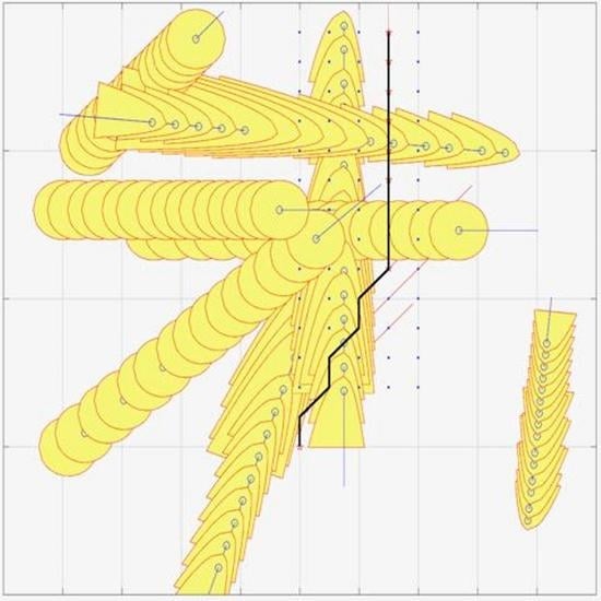
A computer simulation of the DT algorithm is carried out in the MATLAB/Simulink software using an example of a real navigational situation of passing eight encountered ships in the Skagerrak–Kattegat Straits, registered by the ARPA radar on the research and training vessel r/v HORYZONT II (

Table 2. Data describing the situation of one’s own ship passing by eight encountered ships.

Ship j	Distance Dj (nm)	Bearing Nj (o)	Speed Vj (kn)	Course ψj (o)
0–one’s own ship	-	-	20	0
1	8.8	326	13.5	90
2	14.3	6	16.2	180
3	7.5	11	16	200
4	12.1	35	15.7	275
5	7.8	270	14.3	50
6	8.1	108	7.9	6
7	11.3	315	9.6	90
8	12.4	325	6.7	45

and Figure 11, Figure 12 and Figure 13).

The shape of the domain has a significant impact on the course of the ship’s safe trajectory and its final deviation from the set trajectory. The use of a domain in the form of a parabola increases the safety of anti-collision maneuvering at the cost of increasing the final trajectory deviation from the initial value.

3.2. Game Positional Trajectory Algorithm GPT

For the synthesis of safe ship control, a model of a differential game is used. This model is reduced to a positional game of many participants cooperating or not cooperating with each other [49,50,51,52,53,54].

To determine the optimal control of one’s own ship, the sets of acceptable strategies for the passed j ships in relation to one’s own ship must be defined first, followed by sets of acceptable strategies for one’s own ship in relation to each of the j passed ships [55,56,57,58].

The optimal cooperative positioning strategy for one’s own ship is then calculated from the following condition:

$${\mathrm{I}}^{\ast }=\underset{{\mathrm{V}}_0,{\mathsf{\psi }}_0}{\mathrm{m}\mathrm{i}\mathrm{n}}\hspace{0.17em}\hspace{0.17em}\hspace{0.17em}\hspace{0.17em}\underset{{\mathrm{V}}_{\mathrm{j}},{\mathsf{\psi }}_{\mathrm{j}}}{\mathrm{m}\mathrm{i}\mathrm{n}}\hspace{0.17em}\hspace{0.17em}\hspace{0.17em}\hspace{0.17em}\underset{{\mathrm{V}}_0^{\mathrm{j}},{\mathsf{\psi }}_0^{\mathrm{j}}}{\mathrm{m}\mathrm{i}\mathrm{n}}\hspace{0.17em}\hspace{0.17em}\mathrm{I}\hspace{0.17em}\hspace{0.17em}[\mathrm{X},\hspace{0.17em}\mathrm{Y},\hspace{0.17em}\mathrm{P}]={\mathrm{d}}^{\ast }$$

(5)

and the optimal non-cooperative positioning strategy of one’s own ship is calculated from the following condition:

$${\mathrm{I}}^{\ast }=\underset{{\mathrm{V}}_0,{\mathsf{\psi }}_0}{\mathrm{m}\mathrm{i}\mathrm{n}}\hspace{0.17em}\hspace{0.17em}\hspace{0.17em}\hspace{0.17em}\underset{{\mathrm{V}}_{\mathrm{j}},{\mathsf{\psi }}_{\mathrm{j}}}{\mathrm{m}\mathrm{a}\mathrm{x}}\hspace{0.17em}\hspace{0.17em}\hspace{0.17em}\hspace{0.17em}\underset{{\mathrm{V}}_0^{\mathrm{j}},{\mathsf{\psi }}_0^{\mathrm{j}}}{\mathrm{m}\mathrm{i}\mathrm{n}}\hspace{0.17em}\hspace{0.17em}\mathrm{I}\hspace{0.17em}\hspace{0.17em}[\mathrm{X},\hspace{0.33em}\mathrm{Y},\hspace{0.33em}\mathrm{P}]={\mathrm{d}}^{\ast }$$

(6)

The steering goal function d of one’s own ship is characterized by the final deviation of the determined safe trajectory of the ship from a set trajectory. The principle of calculating the optimal trajectory of your own ship consists of calculating values such as the course and speed that ensure the least loss of time or distance to safely pass the encountered ships at a distance no less safe (D_s), taking into account the ship’s dynamics described by the maneuver advance time.

Figure 14 shows the results of a computer simulation of the algorithm for determining the game positional trajectory (GPT) in the navigational situation of one’s own ship passing by eight encountered ships, under the conditions of good and restricted visibility at sea and with cooperation and lack of cooperation between ships.

The degree of cooperation between ships has a significant impact on the course of the ship’s safe trajectory, to a greater extent than the conditions of visibility at sea. The advantage of the non-cooperative algorithm is to ensure greater safety of the own ship in the event of a navigational error or failure of the propulsion system of one of the encountered ships.

3.3. Game Risk Trajectory Algorithm GRT

Apart from the equations for the dynamics of one’s own ship, the differential game model of the collision avoidance process is reduced to a multi-participant matrix game [59,60,61,62,63,64].

In the matrix game, the OS player (one’s own ship) and the ES players (encountered ships) have a number of pure strategies at their disposal in the form of a single course or speed change maneuver. Limitations regarding the choice of strategy result from the COLREGs rules. Most often, the game does not have a saddle point in terms of its solution through the use of pure strategies. Triple linear programming can be used to solve this problem. According to [65,66], in this game, the OS participant seeks to minimize the risk of collision, while the ES participant seeks to minimize or maximize the risk of collision. The components of the mixed strategy of the game participants express the probability distribution of their pure strategies.

Thus, for the cooperative passage of ships, the criterion of safe maneuvering will take the following form:

$${\mathrm{I}}^{\ast }=\underset{{\mathrm{V}}_0,{\mathsf{\psi }}_0}{\mathrm{m}\mathrm{i}\mathrm{n}}\hspace{0.17em}\hspace{0.17em}\hspace{0.17em}\hspace{0.17em}\underset{{\mathrm{V}}_{\mathrm{j}},{\mathsf{\psi }}_{\mathrm{J}}}{\mathrm{m}\mathrm{i}\mathrm{n}}\hspace{0.17em}\hspace{0.17em}\hspace{0.17em}{\mathrm{r}}_{\mathrm{j}}$$

(7)

and for non-cooperation between ships, the criterion will take this form:

$${\mathrm{I}}^{\ast }=\underset{{\mathrm{V}}_0,{\mathsf{\psi }}_0}{\mathrm{m}\mathrm{i}\mathrm{n}}\hspace{0.17em}\hspace{0.17em}\hspace{0.17em}\hspace{0.17em}\underset{{\mathrm{V}}_{\mathrm{j}},{\mathsf{\psi }}_{\mathrm{J}}}{\mathrm{m}\mathrm{a}\mathrm{x}}\hspace{0.17em}\hspace{0.17em}\hspace{0.17em}{\mathrm{r}}_{\mathrm{j}}$$

(8)

As a result, a probability matrix using particular pure strategies is obtained. The solution to the problem of safe control is the strategy with the highest probability.

Figure 15 shows the results of the computer simulation of the algorithm for determining the game risk trajectory (GRT) in the navigational situation of one’s own ship passing by eight encountered ships under the conditions of good and restricted visibility at sea and with cooperation and lack of cooperation between ships.

The collision risk algorithm is the most sensitive to changes in the approaching distance of ships. Particularly large deviations in the trajectory occur in conditions of restricted visibility at sea and from lack of cooperation between ships.

3.4. Kinematic Trajectory Algorithm KT

If the encountered ships do not maintain their given course and speed while maneuvering, then the control quality criterion (3) for non-game kinematic optimization takes the following form:

$${\mathrm{I}}^{\ast }=\underset{{\mathrm{V}}_0,{\mathsf{\psi }}_0}{\mathrm{m}\mathrm{i}\mathrm{n}}\hspace{0.17em}\mathrm{I}\hspace{0.17em}[\mathrm{X},\hspace{0.17em}\mathrm{Y},\hspace{0.17em}\mathrm{P}]={\mathrm{d}}^{\ast }$$

(9)

Figure 16 shows the results of the computer simulation of the algorithm for determining the kinematic trajectory (KT) in the navigational situation of one’s own ship passing by eight encountered ships under good and restricted visibility at sea.

The kinematic trajectory assumes that the encountered ships maintain constant values for courses and speeds. This solution is equivalent to a simple maneuver necessary in the sequential version.

3.5. Comparison of Algorithms

Figure 17 illustrates a comparison of safe own ship trajectories determined according to individual algorithms, separately, for good and restricted visibility conditions.

4. Discussion

Using the ARPA system, the navigator can only designate a single avoidance maneuver against the most dangerous vessel encountered.

The use of the DT algorithm also allows one to calculate the trajectory as a sequence of subsequent maneuvers in relation to all tracked ships, thereby ensuring the smallest deviation from the set cruise route. As the ship is characterized by smaller dynamics of course changes than speed changes, safe time-optimal control is obtained in the first place by changing the course by tilting the rudder. In a situation where more ships are passing by, it is more difficult to determine the optimal and safe trajectory when steering only with the rudder. In that case, the speed can be reduced by reducing the rotational speed of the ship’s propeller. The calculation time of the DT algorithm ranges from a few to several seconds, depending on the number of tracked objects—the more tracked ships, the more nodes in the dynamic programming grid rejected by the NEURAL DOMAINS procedure, and the shorter the calculation time.

In situations where many ships pass each other with limited visibility at sea and in limited waters, both the subjectivity of the navigator in assessing the situation and the high randomness of events are of great importance. In this way, the theory of differential games serves as an ideal theory for solving conflict situations, allowing us to develop appropriate models for positional and matrix games.

Algorithms for determining the game positional trajectory (GPT) and game risk trajectory (GRT) take into account the COLREGs when starting the game, the time of maneuver advance, and the degree of cooperation between ships. The game ends when the collision risk is zero.

5. Conclusions

An important new solution in relation to the existing ones is the use of radar remote sensing in the marine environment together with artificial intelligence methods in the form of an artificial neural network and simplified models of differential games that allow for the synthesis of computer programs supporting the navigator’s control and take into account their subjective assessment of the situation and the ability to maneuver other ships. The computer control algorithms presented in this paper take into account the legal rules of COLREGs maneuvering, as well as the maneuver advance time, and evaluate the final deviation of the safe trajectory from the set trajectory.

The presented computer algorithms for determining the ship’s safe trajectory use radar data from the ARPA system. The calculated safe trajectory of the ship can be simulated on the ARPA system display as an additional function. The neural networks presented in this article enable the representation of heuristic knowledge that is equal to the knowledge of an experienced navigator. However, it remains important to use the knowledge of experienced navigators in teaching the network.

Future work should perform a sensitivity analysis of safe ship control to change the parameters of the control process models and to correct inaccuracies in remote sensing information. In addition, the design of the ARPA system could be extended with an additional function that generates a computer-assisted decision for the maneuvering navigator using an algorithm that connects the game with a neural network.

References

- Lazarowska, A. Safe Trajectory Planning for Maritime Surface Ships; Springer: Berlin/Heidelberg, Germany, 2022; Volume 13, pp. 1–185. [Google Scholar] [CrossRef]
- Li, J.; Zhang, G.; Shan, Q.; Zhang, W. A Novel Cooperative Design for USV-UAV Systems: 3D Mapping Guidance and Adaptive Fuzzy Control. IEEE Trans. Control. Netw. Syst. 2022, 11, 1–11. [Google Scholar] [CrossRef]
- Zhong, S.; Wen, Y.; Huang, Y.; Cheng, X.; Huang, L. Ontological Ship Behavior Modeling Based COLREGs for Knowledge Reasoning. J. Mar. Sci. Eng. 2022, 10, 203. [Google Scholar] [CrossRef]
- Kim, H.-G.; Yun, S.-J.; Choi, Y.-H.; Ryu, J.-K.; Suh, J.-H. Collision Avoidance Algorithm Based on COLREGs for Unmanned Surface Vehicle. J. Mar. Sci. Eng. 2021, 9, 863. [Google Scholar] [CrossRef]
- Zhang, G.; Li, J.; Liu, C.; Zhang, W. A robust fuzzy speed regulator for unmanned sailboat robot via the composite ILOS guidance. Nonlinear Dyn. 2022, 110, 2465–2480. [Google Scholar] [CrossRef]
- Zhou, X.; Huang, J.; Wang, F.; Wu, Z.; Liu, Z. A Study of the Application Barriers to the Use of Autonomous Ships Posed by the Good Seamanship Requirement of COLREGs. J. Navig. 2020, 73, 710–725. [Google Scholar] [CrossRef]
- Lebkowski, A. Evolutionary methods in the management of vessel traffic. In Proceedings of the International Conference on Marine Navigation and Safety of Sea Transportation, Gdynia, Poland, 17–19 June 2015; pp. 259–266. [Google Scholar]
- Borkowski, P. The Ship Movement Trajectory Prediction Algorithm Using Navigational Data Fusion. Sensors 2017, 17, 1432. [Google Scholar] [CrossRef]
- Tomera, M. Ant Colony Optimization Algorithm Applied to Ship Steering Control. 18th Annual International Conference on Knowledge-Based and Intelligent Information and Engineering Systems KES, Gdynia, Poland. Procedia Comput. Sci. 2014, 35, 83–92. [Google Scholar] [CrossRef] [Green Version]
- Pietrzykowski, Z.; Wołejsza, P. Decision support system in marine navigation. In Challenge of Transport Telematics, Proceedings of the 16th International Conference on Transport Systems Telematics, Katowice-Ustroń, Poland, 16–19 March 2016; Springer: Berlin/Heidelberg, Germany, 2016; Volume 640, pp. 462–474. [Google Scholar] [CrossRef]
- Ożoga, B.; Montewka, J. Towards a decision support system for maritime navigation on heavily trafficked baśni. Ocean Eng. 2018, 159, 88–97. [Google Scholar] [CrossRef]
- Aylward, K.; Weber, R.; Lundh, M.; MacKinnin, S.N.; Dahlman, J. Navigators’ views of a collision avoidance decision support system for maritime navigation. J. Navig. 2022, 75, 1035–1048. [Google Scholar] [CrossRef]
- Szlapczynski, R.; Szlapczynska, J. A method of determining and visualizing safe motion parameters of a ships navigating in restricted waters. Ocean. Eng. 2017, 129, 363–373. [Google Scholar] [CrossRef]
- Hongguang, L.; Yong, Y. Fast Path Planning for Autonomous Ships in Restricted Waters. Appl. Sci. 2018, 12, 2592. [Google Scholar] [CrossRef] [Green Version]
- Wei, D.; Langxiong, G.; Chunhui, Z.; Yuanzhou, Z.; Mingjuan, L.; Lei, Z. Study on Path Planning of Ship Collision Avoidance in Restricted Water base on AFS Algorithm. In Proceedings of the 27th International Ocean and Polar Engineering Conference, San Francisco, CA, USA, 25–30 June 2017; pp. 1–7. [Google Scholar]
- Dinh, G.H.; Im, N.K. Study on the Construction of Stage Discrimination Model and Consecutive Waypoints Generation Method for Ship’s Automatic Avoiding Action. Int. J. Fuzzy Log. Intell. Syst. 2017, 17, 294–306. [Google Scholar] [CrossRef] [Green Version]
- Hinostroza, M.A.; Xu, H.; Soares, C.G. Cooperative operation of autonomous surface vehicles for maintaining formation in complex marine environment. Ocean Eng. 2019, 183, 132–154. [Google Scholar] [CrossRef]
- Hongguang, L.; Yong, Y. COLREGS-Constrained Real-time Path Planning for Autonomous Ships Using Modified Artificial Potential Fields. J. Navig. 2018, 72, 588–608. [Google Scholar] [CrossRef]
- Lisowski, J. The dynamic game models of safe navigation. TransNav Int. J. Mar. Nav. Safety Sea Transp. 2007, 1, 11–18. [Google Scholar]
- Sun, Z.; Sun, H.; Li, P.; Zou, J. Self-organizing cooperative pursuit strategy for multi-USV with dynamic obstacle ships. J. Mar. Sci. Eng. 2022, 10, 562. [Google Scholar] [CrossRef]
- Engwerda, J. Stabilization of an uncertain simple fishery management game. Fish. Res. 2018, 203, 63–73. [Google Scholar] [CrossRef] [Green Version]
- Singh, S.K.; Reddy, P.V. Dynamic network analysis of a target defense differential game with limited observations. arXiv 2021, arXiv:2101.05592. [Google Scholar]
- Mu, C.; Wang, K.; Ni, Z.; Sun, C. Cooperative differential game-based optimal control and its application to power systems. IEEE Trans. Ind. Inform. 2020, 16, 5169–5179. [Google Scholar] [CrossRef]
- Huang, Y.; Zhang, T.; Zhu, Q. The inverse problem of linear-quadratic differential games: When is a control strategies profile Nash? arXiv 2022, arXiv:2207.05303. [Google Scholar]
- Gronbaek, L.; Lindroos, M.; Munro, G.; Pintassilgo, P. Cooperative Games in Fisheries with More than Two Players. In Game Theory and Fisheries Management; Springer: Cham, Switzerland, 2020; pp. 81–105. ISBN 978-3-030-40112-2. [Google Scholar]
- Gromova, E.V.; Petrosyan, L.A. On an approach to constructing a characteristic function in cooperative differential games. Project: Cooperative differential games with applications to ecological management. Autom. Remote Control 2017, 78, 1680–1692. [Google Scholar] [CrossRef]
- Basar, T.; Olsder, G.J. Dynamic Non-Cooperative Game Theory; Siam: Philadelphia, PA, USA, 2013; ISBN 978-0-898-714-29-6. [Google Scholar]
- Rocha, A.F. Neural Nets—Theory of Brain a Machines; Springer: Berlin/Heidelberg, Germany; New York, NY, USA, 1992; ISBN 0-8493-2643-5. [Google Scholar]
- Hwang, J.I.; Chae, S.H.; Kim, D.; Jung, H.S. Application of Artificial Neural Networks to Ship Detection from X-Band Kompsat-5 Imagery. Appl. Sci. 2017, 7, 961. [Google Scholar] [CrossRef]
- Kang, M.; Ji, K.; Leng, X.; Lin, Z. Contextual Region-Based Convolutional Neural Network with Multilayer Fusion for SAR Ship Detection, Remote Sens. 2017, 9, 860. Remote Sens. 2017, 9, 860. [Google Scholar] [CrossRef] [Green Version]
- Collingwood, A.; Treitz, P.; Charbonneau, F.; Atkinson, D.M. Artificial Neural Network Modeling of High Arctic Phytomass Using Synthetic Aperture Radar and Multispectral Data. Remote Sens. 2014, 6, 2134–2153. [Google Scholar] [CrossRef] [Green Version]
- Colley, B.A.; Curtis, R.G.; Stockel, C.T. Manoeuvring Times, Domains and Arenas. J. Navig. 1983, 36, 324–328. [Google Scholar] [CrossRef]
- Davis, P.V.; Dove, M.J.; Stockel, C.T. A computer simulation of marine traffic using domains and areas. J. Navig. 1980, 33, 215–222. [Google Scholar] [CrossRef]
- Goodvin, E.M.A. Statistical study of ship domains. J. Navig. 1975, 28, 328–334. [Google Scholar] [CrossRef] [Green Version]
- Stateczny, A. Neural Manoeuvre Detection of the Tracked Target in ARPA Systems. In Proceedings of the IFAC Conference on Control Applications in Marine Systems, Glasgow, Scotland, 19–21 June 2011; pp. 209–214. [Google Scholar]
- Wlodarczyk-Sielicka, M.; Lubczonek, J.; Stateczny, A. Comparison of selected clustering algorithms of raw data obtained by interferometric methods using artificial neural networks. In Proceedings of the 17th International Radar Symposium, Krakow, Poland, 10–12 May 2016. [Google Scholar]
- Hertz, J.; Krogh, A.; Palmer, R.G. Introduction to the Theory of Neural Computation; CRC Press: Boca Raton, FL, USA, 2018; ISBN 978-0-201-51560-1. [Google Scholar]
- Lisowski, J. The optimal and safe ship trajectories for different forms of neural state constraints. Mechatr. Syst. Mech. Mater. 2012, 180, 64–69. [Google Scholar] [CrossRef]
- Bellman, R.E. Dynamic Programming; Dover Publication: New York, NY, USA, 2003; ISBN 0-486-42809-5. [Google Scholar]
- Lew, A.; Mauch, H. Dynamic Programming–A Computational Tool; Springer: Berlin, Germany, 2007; ISBN 978-3-540-37014-7. [Google Scholar]
- Geng, X.; Wang, Y.; Wang, P.; Zhang, B. Motion of maritime autonomous surface ships by dynamic programming for collision avoidance and speed optimization. Sensors 2019, 19, 434. [Google Scholar] [CrossRef] [Green Version]
- Witkowska, A.; Smierzchalski, R. Adaptive Dynamic Control Allocation for Dynamic Positioning of Marine Vessel Based on Backstepping Method and Sequential Quadratic Program. Ocean Eng. 2018, 163, 570–582. [Google Scholar] [CrossRef]
- Guenin, B.; Konemann, J.; Tuncel, L.A. Gentle Introduction to Optimization; Cambridge University Press: Cambridge, UK, 2014; ISBN 978-1-107-05344-1. [Google Scholar]
- Speyer, J.L.; Jacobson, D.H. Primer on Optimal Control Theory; SIAM: Toronto, ON, Canada, 2010; ISBN 978-0-898716-94-8. [Google Scholar]
- Yong, J. Optimization Theory–A Concise Introduction; World Sc.: New York, NY, USA, 2018; ISBN 978-981-3237-64-3. [Google Scholar]
- Ehrgott, M.; Gandibleux, X. Multiple Criteria Optimization: State of the Art Annotated Bibliographic Surveys; Kluwer Academic Press: New York, NY, USA, 2002. [Google Scholar]
- Marler, R.T.; Arora, J.S. Survey of multi-objective optimization methods for engineering. Struct. Multidiscip. Optim. 2004, 26, 369–395. [Google Scholar] [CrossRef]
- Legriel, J. Multicriteria Optimization and Its Application to Multi-Processor Embedded Systems. Ph.D. Thesis, Grenoble University, Grenoble, France, 2011. [Google Scholar]
- Isaacs, R. Differential Games; John Wiley & Sons: New York, NY, USA, 1965; ISBN 0-48640-682-2. [Google Scholar]
- Hunt, K.J.; Irwin, G.R.; Warwick, K. Neural Network Engineering in Dynamic Control Systems; Advances in Industrial Control Series; Springer: Berlin, Germany, 1995; ISBN 3-540-19973-X. [Google Scholar]
- Leondes, C.T. Control and Dynamic Systems, Neural Network Systems Techniques and Applications; Academic Press: New York, NY, USA, 1998; Volume 7, ISBN 978-0124438675. [Google Scholar]
- Francelin, R.; Kacprzyk, J.; Gomide, F. Neural Network Based Algorithm for Dynamic System Optimization. Asian J. Contr. 2001, 3, 131–142. [Google Scholar] [CrossRef]
- Braquet, M.; Bakolas, E. Vector field-based collision avoidance for moving obstacles with time-varying elliptical shape. arXiv 2022, arXiv:2207.01747v2. Available online: https://arxiv.org/pdf/2207.01747.pdf (accessed on 19 December 2022).
- Chen, Y.; Georgiou, T.T.; Pavon, M. Covariance steering in zero-sum linear-quadratic two-player differential games. arXiv 2019, arXiv:1909.05468v1. Available online: https://arxiv.org/pdf/1909.05468.pdf (accessed on 20 December 2022).
- Engwerda, J.C. LQ Dynamic Optimization and Differential Games; John Wiley & Sons: New Jork, NY, USA, 2005; ISBN 978-0-470-01524-7. [Google Scholar]
- Hermes, H.; Isaacs, R. Differential Games. Math. Comput. 1965, 19, 700. [Google Scholar] [CrossRef]
- Li, Y.; Vorobeychik, Y. Path planning games. Multiagent Syst. arXiv 2019, arXiv:1910.13880. [Google Scholar]
- Osborne, M.J. An Introduction to Game Theory; Oxford University Press: New York, NY, USA, 2004; ISBN 978-0-19-512895-6. [Google Scholar]
- Spica, R.; Cristofalo, E.; Wang, Z.; Montijano, E.; Schwager, M. A Real-Time Game Theoretic Planner for Autonomous Two-Player Drone Racing. IEEE Trans. Robot. 2020, 36, 1389–1403. [Google Scholar] [CrossRef]
- Wells, D. Game and Mathematics; Cambridge University Press: London, UK, 2003; ISBN 978-1-78326-752-1. [Google Scholar]
- Millington, I.; Funge, J. Artificial Intelligence for Games; CRC Press: Boca Raton, FL, USA, 2018. [Google Scholar]
- Nisan, N.; Roughgarden, T.; Tardos, E.; Vazirani, V.V. Algorithmic Game Theory; Cambridge University Press: New York, NY, USA, 2007. [Google Scholar]
- Hosseinzadeh, M.; Garone, E.; Schenato, L. A Distributed method for linear programming problems with box constraints and time-varying inequalities. IEEE Control Syst. Lett. 2018, 3, 404–409. [Google Scholar] [CrossRef]
- Liu, Z.; Wu, Z.; Zheng, Z. A cooperative game approach for assessing the collision risk in multi-vessel encountering. Ocean Eng. 2019, 187, 106175. [Google Scholar] [CrossRef]
- Lisowski, J. Game Control Methods Comparison when Avoiding Collisions with Multiple Objects Using Radar Remote Sensing. Remote Sens. 2020, 12, 1573. [Google Scholar] [CrossRef]
- Lisowski, J. Sensitivity of computer support game algorithms of a safe ship control. Int. J. Appl. Math. Comput. Sci. 2013, 23, 439–446. [Google Scholar] [CrossRef]
Figure 1.
Graphical presentation of the functioning of the navigator support system tested on a research and training vessel r/v HORYZONT II in a real marine environment in the Skagerrak–Kattegat Straits: V, ψ is the speed and course of one’s own ship; Vj, ψj is the encountered j ship speed and course; Dj, Nj is the distance and bearing to j the encountered ship; D is the safe passing distance for ships in real conditions of visibility at sea; Djmin, Tjmin is the distance and time to the closest approach of the ships.
Figure 2.
Structure of the decision support system.
Figure 3.
Diagram of standard Raytheon Anschutz radar system interfaces.
Figure 4.
The format of the data frame with the sample parameters of one’s own ship.
Figure 5.
The format of the data frame containing the sample information about the tracked ship.
Figure 6.
Neural network evaluating the risk of collision with j encountered ship and determining the size of the passing ship domain: wmn, w′mn, and w′′mn neuron weights of the first, second, and third layers, respectively.
Figure 7.
The navigation situation presented to the navigator as the teacher of the neural network.
Figure 8.
The mean square error of the learning process of a neural network assessing the risk of ship collision.
Figure 9.
The shape of the neural collision risk domains in the situation of four encountered ships.
Figure 10.
Flow chart of the DT algorithm for calculating the ship’s safe dynamic trajectory in a collision situation using marine environment radar remote sensing data.
Figure 11.
Illustrating the navigation situation in the form of twelve-minute speed vectors of one’s own ship and eight encountered ships.
Figure 12.
Safe dynamic trajectory of one’s own ship determined by the DT algorithm with neural domains of passing ships in the forms of circles, hexagons, ellipses, and parabolas under conditions of good visibility at sea at different values of the adopted safe passing distance Ds; t* is the optimal time to avoid a collision situation.
Figure 13.
Safe dynamic trajectory of one’s own ship determined by the DT algorithm with neural domains of passing ships in the forms of circle, hexagons, ellipses, and parabolas with restricted visibility at sea at different values of the adopted safe passing distance Ds; t* is the optimal time to avoid a collision situation.
Figure 14.
Safe game positional trajectory of one’s own ship determined by the GPT algorithm, in good (gw) and restricted (rw) visibility at sea, with cooperation of vessels (c) and non-cooperation between vessels (nc); d* means the final deviation of the ship’s own course from the initial value after exiting the collision situation.
Figure 15.
Safe game risk trajectory of one’s own ship determined by the GRT algorithm, in good (gw) and restricted (rw) visibility at sea, with the cooperation of vessels (c) and non-cooperation between vessels (nc); d* means the final deviation of the course of one’s own ship from the initial value after exiting the collision situation.
Figure 16.
Safe kinematic trajectory of one’s own ship determined by the KT algorithm, in good (gw) and restricted (rw) visibility at sea; d* means the final deviation of the course of one’s own ship from the initial value after exiting the collision situation.
Figure 17.
Safe ship trajectories determined according to DT, GPT, GRT, and KT algorithms for good visibility at sea (left) and restricted visibility at sea (right) conditions.