Optimization of Characteristic Phenological Periods for Winter Wheat Extraction Using Remote Sensing in Plateau Valley Agricultural Areas in Hualong, China

Abstract

It is important to develop or validate remote sensing methods to explore agricultural management and food self-sufficiency in the agricultural areas of the Qinghai–Tibet Plateau under the influence of global change, ecological protection, and socio-economic development. Studies on the use of remote sensing to monitor crop planting on the Qinghai-Tibetan Plateau are limited, with inconclusive results. Therefore, in this study, we analyzed Sentinel-2A/B images and field survey data in Hualong, China (located in Hehuang Valley, Qinghai-Tibetan Plateau) for winter wheat identification and verification at different spatial scales based on the time series of the normalized difference phenology index (NDPI) and dynamic time warping (DTW) algorithm. The characteristic phenological period and the corresponding DTW threshold were optimized using remote sensing data extracted for winter wheat. The results showed that NDPI corresponding to the jointing-heading stage, grouting-harvesting stage, and jointing-harvesting stage with DTW could identify winter wheat regardless of whether the spatial scale was a single quadrat, a combination of two quadrats, or the entire study area. The NDPI corresponding to the jointing-heading stage (corresponding DTW threshold T = 0.158) could generate a relatively rational winter wheat map; the NDPI corresponding to the time series of the grouting-harvesting stage (combined with DTW threshold T = 0.195) could detect a planting area with relatively high accuracy when supported by cultivated land, which matches the statistical reporting of the winter wheat area data. Similarly, with the support of cultivated land data, the planted area could be identified early based on the phenological characteristics of winter wheat before overwintering; however, the extraction scheme needs to be optimized further.

1. Introduction

It is important to timely and accurately obtains the winter wheat planting area and its spatiotemporal variation to maximize the production potential of winter wheat, promote the sustainable and efficient development of agricultural production, and ensure food security [1]. Remote sensing technology for the observation of the earth has become the main method of extracting information from crop planting owing to its outstanding application advantages [2]. Among them, spectral features, temporal features, and spatial features have been widely studied for crop mapping [3]. Most machine-learning approaches use a single remote-sensing image with spectral or spatial features for extraction [4]. However, the spectral characteristics of crops are constantly changing in the growing season, and the phenological periods of different crops often coincide. Single remote sensing images cannot show the spectral characteristics of crop changes that can be seen with time-series remote sensing images [5]. Owing to the availability of high temporal resolution image data, it is possible to use time series remote sensing images or products for crop mapping. Compared with other non-overwintering crops, the time series of the vegetation index of the winter wheat changed more obviously at the tillering to heading stages. Based on this feature, a technical scheme to extract and map winter wheat information by using a time series of vegetation index data was developed [6]. The classification method based on time series remote sensing image data or products makes full use of the characteristics of seasonal changes in crops and the trend characteristics of crop growth over time and can be used as one of the main methods to extract crop planting information [7,8]. Nonetheless, the spatial distribution of crops and the influence of image noise leads to the deviation and distortion of the phenological characteristic curve, which affects crop recognition [9,10,11]. The dynamic time warping (DTW) algorithm was developed to measure the similarity of two-time series with different lengths [12]. It was initially applied in speech recognition for similarity searches between time series [13] and was later introduced into the field of satellite image time series data analysis. It is used in agricultural remote sensing to match the dislocation of phenological characteristic curves of target crops and reference crops caused by the difference in spatial distribution. Therefore, this method has attracted widespread attention with promising application results [14,15,16,17,18].

The Qinghai–Tibet Plateau (QTP) is called the third pole of the world and is home to almost 10 million people. However, there are few natural areas suitable for agriculture due to the cold geographical environment. From the perspective of food self-sufficiency, the QTP is the main area of grain shortage in China [19] and possibly in the world. A survey of the Second Tibetan Plateau Scientific Expedition and Research shows that farmers’ willingness to plant crops directly affects the scale of crop cultivation and affects grain self-sufficiency under the combined influence of frequent extreme climate/weather events, ecological protection, and economic benefits. Therefore, developing and verifying real-time monitoring methods for crop planting in the QTP is important to understand the spatial patterns and areas of crop planting.

The Hehuang Valley in the northeast of the QTP and the YNL basin (the Yarlung Zangbo River with its two tributaries, the Nyangqu River and the Lhasa River) in Tibet have formed unique plateau agricultural areas due to local environmental conditions and are the two major grain production centers in the QTP [19]. The two agricultural areas support over two-thirds (>6 million) of the QTP population. As an ecological zone sensitive to global change, monitoring vegetation changes by remote sensing has received much attention from scholars. Existing studies on agricultural production in this region have focused mainly on the temporal and spatial evolution of cultivated land, the response of the planting structure to climate change, and the macro prediction of grain yield [20,21,22]. This region is not the main agricultural production area on a global or national scale, and as there are few monitoring stations, there is a lack of data. Furthermore, regressive technology development and the missing or irregular availability of information have resulted in reduced remote sensing-based crop planting monitoring. Huang et al. [23] compared and optimized the normalized difference phenology index (NDPI) as the best time series vegetation index for winter wheat extraction in Minhe, QTP [23]. However, the seeding-tillering stage and ripening-harvest stage were empirically selected as characteristic phenological periods according to the differences between the phenological characteristics of winter wheat and other vegetation in the study area [23]. There may be large differences in winter wheat growth during sowing and overwintering at the temporal and spatial scales due to inter-region and inter-year fluctuations in climate conditions in autumn and winter [24,25]. Therefore, further verification is needed to determine whether the selected phenological period from the previous study [23] is optimal for further promotion and application in plateau valley areas with larger planting areas and more complex planting conditions.

To address the above problems, we studied the plateau valley area in Hualong, China, to optimize the characteristic phenological period of winter wheat extracted by remote sensing. Using remote sensing image data, field survey data, administrative division data, and the statistical reporting of winter wheat area data, the results of winter wheat planting information extracted from remote sensing images were compared under different combinations of phenological periods on the quadratic scale based on the NDPI and DTW. The combination of phenological periods and their threshold values for winter wheat identification were optimized and verified on an overall scale. This provides a reference for exploring agricultural production management and food self-sufficiency in the plateau region under the influence of global change, ecological protection, and socio-economic development.

2. Materials and Methods

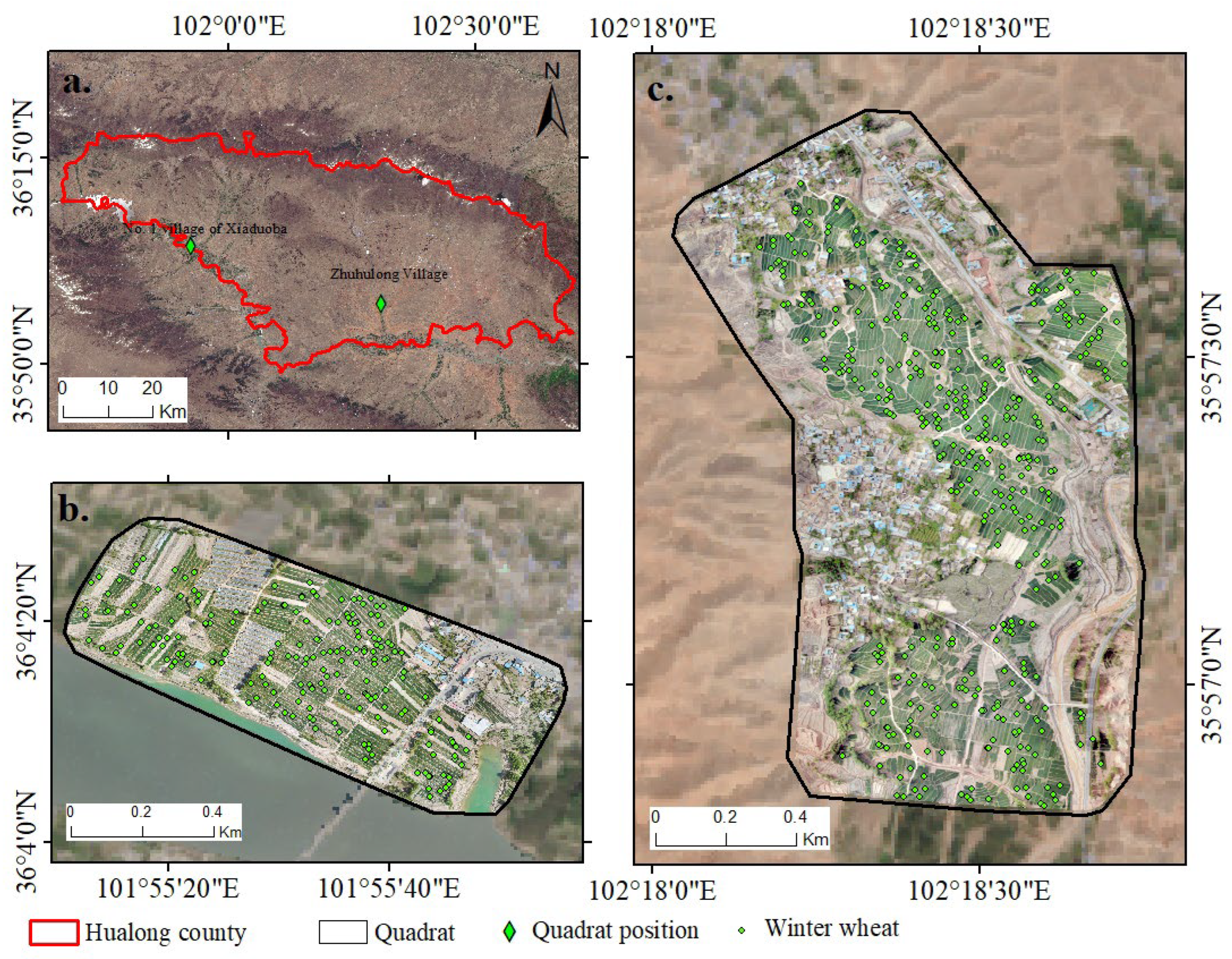
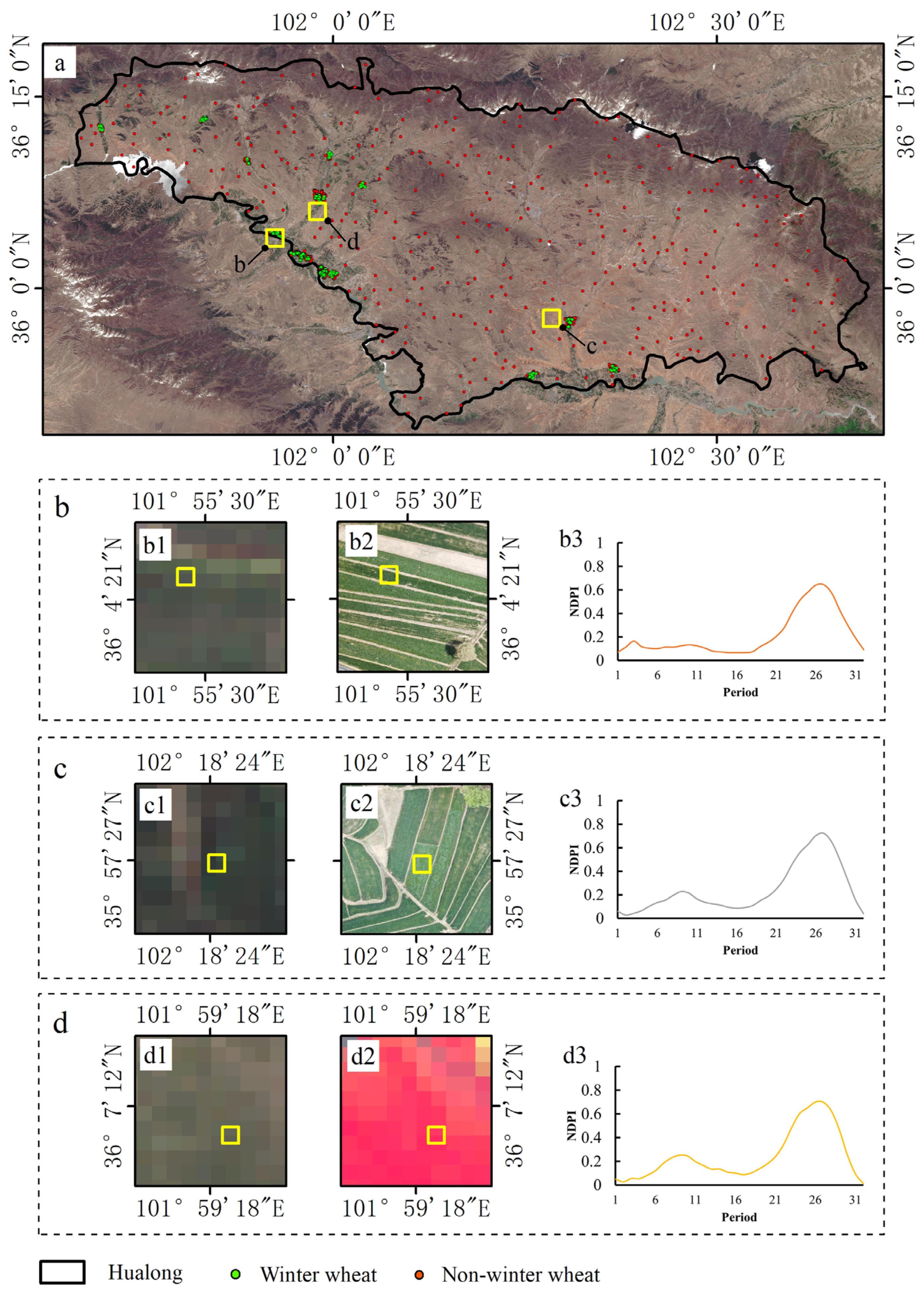
2.1. Study Area

Hualong, China, is a semi-agricultural and semi-pastoral area in the south of the Hehuang Valley, in the transition zone between the Loess Plateau and the QTP. The total area is approximately 2740 km², and its altitude is between 1884 and 4484 m. This area is dominated by crisscrossing mountainous valleys, and the terrain slopes from northwest to the southwest [26]. The Yellow River flows along its southern margin (Figure 1), and this area has abundant sunshine with little precipitation. The annual average temperature is only 2.2 °C, and the frost-free period is short. Crops mainly include cold and drought-tolerant wheat, barley, potatoes, peas, rape, and flax. It is a typical agricultural area in the plateau valley or winter wheat planting edge area. Winter wheat is only distributed on river valley terraces that can meet the needs of its hydrothermal combination.

The winter wheat planting area in Hualong has increased from approximately 500 mu (33.3 ha) at the end of the last century to one of the largest winter wheat production areas in Qinghai, China, due to climate warming, increased precipitation, and the active guidance of the agricultural management department [27,28]. The planting of winter wheat in Hualong occurred primarily in three towns (Gandu, Qunke, and Yashiga) from 2017 to 2020, with a total area of approximately 40,000 mu (2800 ha); this accounted for approximately 30% of the sown area according to the public broadcast data provided by the Ministry of Agriculture and Rural Affairs [29,30,31,32]. Therefore, this area is suitable for exploring the remote sensing extraction method for winter wheat, which can also lay a foundation for routine monitoring in the Hehuang Valley.

2.2. Data

2.2.1. Satellite Remote Sensing Data

Sentinel-2A/B MSI data were used due to its spatial, temporal, and spectral resolution, especially in regions with complex geographical environments and broken farmland [33,34], which can be observed in the study area. The Google Earth Engine (GEE, http://earthengine.google.com (accessed on 15 December 2022)) integrates massive remote sensing data, including Sentinel satellite data, and provides algorithm compilation functions for rapid data processing and analysis. Atmospherically corrected Sentinel-2A/B MSI data from August 2020 to August 2021 were directly acquired through the GEE, and subsequent data processing was conducted based on the GEE.

2.2.2. Field Survey Data

Field investigations were conducted to gain real samples and assist in the construction of the NDPI reference curve. Point data of surface vegetation types and two high-resolution quadrat image datasets were obtained using a DJI Mavic2 ZOOM UAV. Point data were collected in May 2021, the UAV remote sensing data acquisition date was 2 May 2021, and the flight altitude was 117 m. The true color ortho image with a spatial resolution of 4.35 cm was obtained through the correction and fusion of the original data (Figure 2). Quadrat 1 (Figure 2b) is located in the No. 1 village of Xiaduoba, Yashiga Town, Hualong County. The winter wheat planting area is 272 mu (19.04 ha), which is 35% of the effective data coverage. Quadrat 2 (Figure 2c) is located in Zhuhulong Village, Gandu Town, Hualong County. The planting area is 526 mu (36.82 ha), which represents 22% of the effective data coverage.

2.2.3. Administrative Division Data

The study area is bound by the Hualong, China, vector boundary, derived from the 1:1,000,000 national basic geographic database of the National Catalogue Service for Geographic Information [35].

2.2.4. Planting Data

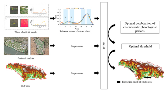
The planting data is the winter wheat planting area in Hualong, obtained from the statistical report data on the official website of the Ministry of Agriculture and Rural Affairs of the People’s Republic of China (http://www.moa.gov.cn (accessed on 15 December 2022)). These data were used to statistically analyze the winter wheat identification area in the study area.

2.3. Methods

2.3.1. Vegetation Index

The vegetation index of a time series reflects the growth rhythm of plants and their phenological characteristics [36]. Land use/cover change can be inferred from the phenological differences in the underlying surfaces; therefore, this approach is widely applied in crop distribution monitoring [37]. Time series NDPI combined with DTW has proved effective at extracting winter wheat in the main producing areas and marginal areas [23,38]. Therefore, this study selected NDPI (Equation (1)) to optimize the characteristic phenological period and to verify its generalizability for winter wheat extraction in agricultural areas of the plateau valley.

$$\begin{array}{c}\mathrm{NDPI}=\frac{\left(\mathrm{NIR}-\left(0.74\times \mathrm{R}+\left(1-0.74\right)\times \mathrm{SWIR}\right)\right)}{\left(\mathrm{NIR}+\left(0.74\times \mathrm{R}+\left(1-0.74\right)\times \mathrm{SWIR}\right)\right)}\end{array}$$

(1)

where NIR corresponds to band B8 from Sentinel-2A/B MSI data, R corresponds to band B4 Sentinel-2A/B MSI data, and SWIR corresponds to band B11 Sentinel-2A/B MSI data.

2.3.2. Quality Mosaic Cloud Removal

Mosaic cloud removal is a necessary preprocessing step for optical remote-sensing images. GEE provides a cloud removal algorithm for Sentinel-2A/B images, but its principle is to eliminate pixels with cloud values larger than the threshold value. In this paper, the two adjacent phases of images are combined into one phase. If the cloud removal algorithm is adopted, there may be holes in the generated result; therefore, we adopted the quality mosaic algorithm, which can ensure the continuity of the generated time series. First, a band was selected as the quality band for evaluating the pixel quality, Huang et al. [23] found that using NDVI as the quality band for quality mosaic had a better effect than NDPI and EVI. So, in this article, NDVI was directly selected as the mass band for mosaic cloud removal. Then, the step size was set, and the greater the number of images selected for processing, the better the cloud removal effect and the higher the quality of the obtained image was. However, if the selected step size is too long, the number of generated time series periods is too small, which weakens the curve features and amplifies the differences in vegetation growth features within the region, which may affect the extraction accuracy. Most previous studies have used 10, 15, or 30 days as the step size [39,40,41]. This study chose a 10-day step (two adjacent periods) for the construction of the time series after considering the above factors. The corresponding pixels of all the images in the step size were sorted from high to low according to the quality band. The higher pixel quality of the quality band resulted in higher corresponding image pixel values, and the image pixels corresponding to these high pixel values were the final mosaic output pixel (Appendix A). Cloud-polluted pixels with low-quality band values were replaced with cloud-free pixels during sorting.

2.3.3. S-G Filtering

Sensor status, surface environmental fluctuation, and atmospheric interference may create anomalies or noise in time series remote sensing data products [42], which may cause errors in data analysis. This influence of anomalies or noise can be weakened using a data flow smoothing and denoising filtering method, which is used in signal processing [43,44]. Savitzky–Golay (S-G) filtering [45] is widely used in existing studies. It uses a filter of a certain length for a convolution operation and a weighted polynomial fitting to weaken outliers in time series data to optimize the trend line [46,47]. This method has the advantage of retaining the shape and width of the signal while removing noise, is easy to calculate, and has strong operability [48]. Its basic formula is stated below:

$$\begin{array}{c}{Y}_j=\frac{{{\displaystyle \sum }}_{i=-m}^{i=m}\begin{array}{cc}{C}_i\times & Y_{j+i}\end{array}}{N}\end{array}$$

(2)

where $Y_j$ is the S-G filter value, $Y_{j+i}$ is the original value, m is the radius of the filtering window, N is the size of the filtering window, and $C_i$ is the weight of i point.

Setting the radius of the filtering window m and the number d affects the final smoothing effect of the curve. If m is too small, the fitting effect is not obvious, and redundant data are easily generated. If m is too large, some details are easily missed. If d is too small, the fit will be too smooth, and the effect will be poor. If d is too large, overfitting may occur. In most existing studies, d is 2–4, and m is 3–7 [49]. However, considering that the time series with the filtering window (2m + 1) is short, a large value of m may weaken the characteristics of the curve. Therefore, in this study, the S-G filtering of the NDPI time series used intermediate parameter values (d = 3; m = 5).

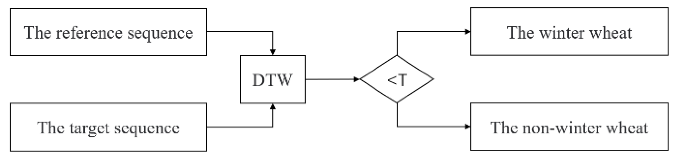
2.3.4. DTW Algorithm

This study selected the DTW algorithm to extract information on winter wheat planting according to the specific implementation process (Appendix B).

• The target and reference sequences were set as T = T{T(1), T(2), …, T(N)} and R = {R(1), R(2), …, R(M)}, where T(n) and R(m) (n$\in \left[1,\mathrm{N}\right]$, m$\in \left[1,\mathrm{M}\right]$) are the n and m eigenvectors of the corresponding sequence, respectively.
• The distance between any two-time series data points is represented by d(T(n), R (m)). The distance function adopts the Euclidean distance, and its formula is stated as follows:

  $$\begin{array}{c}d\left(T\left(\mathrm{n}\right),\mathrm{R}\left(\mathrm{m}\right)\right)=\sqrt{{\left(x\left(n\right)-x\left(m\right)\right)}^2+{\left(y\left(n\right)-y\left(m\right)\right)}^2}\end{array}$$

  (3)
• A search of each path determines the shortest cumulative distance starting from T(N) to R(M) by finding the sum of the minimum distances between each point in T and R. The smaller the shortest cumulative distance is, the more similar T and R are. The threshold of the shortest cumulative distance is set during the extraction of winter wheat in this study. A cumulative distance between the target NDPI and reference NDPI sequences that is less than or equal to this threshold was considered winter wheat; otherwise, it was considered other ground objects (Figure 3).

2.3.5. Receiver Operating Characteristic (ROC) Curve

In the study of land use classification, a confusion matrix is widely used to verify its accuracy. However, this paper only extracts winter wheat from complex backgrounds, and other pixels are classified as non-winter wheat; therefore, it is a binary classification problem. The ROC is often used to evaluate the performance of binary classifiers [50]. It takes the false positive rate (FPR) as the horizontal axis and the true positive rate (TPR) as the vertical axis. The closer the (0,1) point in the upper left corner, the better the threshold extraction result. When evaluating more curves for different classifiers, the classifier corresponding to the upper curve is often better than the lower one, and the evaluation results can be intuitively displayed by the ROC.

TPR and FPR were used to select optimal thresholds in the extraction results of the continuing phenological time series, and accuracy (ACC) was used to evaluate the extraction results of the non-continuous phenological time series (Appendix C). The specific algorithm for each indicator was determined as follows:

$$\begin{array}{c}\mathrm{TPR}=\frac{\mathrm{TP}}{\left(\mathrm{TP}+\mathrm{FN}\right)}\times 100\%\end{array}$$

(4)

$$\begin{array}{c}\mathrm{FPR}=\frac{ \mathrm{FP}}{\left(\mathrm{TN}+\mathrm{FP}\right)}\times 100\%\end{array}$$

(5)

$$\begin{array}{c}\mathrm{ACC}=\frac{\left(\mathrm{TP}+\mathrm{TN}\right)}{\left(\mathrm{TP}+\mathrm{FP}+\mathrm{FN}+\mathrm{TN}\right)}\times 100\%\end{array}$$

(6)

where TP (true positive) is the number of correct classifications of positive samples, FN (false negative) is the number of wrong classifications of positive samples, FP (false positive) is the number of wrong classifications of positive samples, and TN (true negative) indicates the number of correct categories in the negative sample. The positive samples in this study are winter wheat samples, and the negative samples are other samples [51].

3. Process and Results

The phenology optimization process of winter wheat extraction by remote sensing mainly includes: (1) Data processing; (2) Optimizing the combination of characteristic phenological periods and their thresholds; (3) Extracting and validating winter wheat in the study area.

3.1. Data Processing and Results

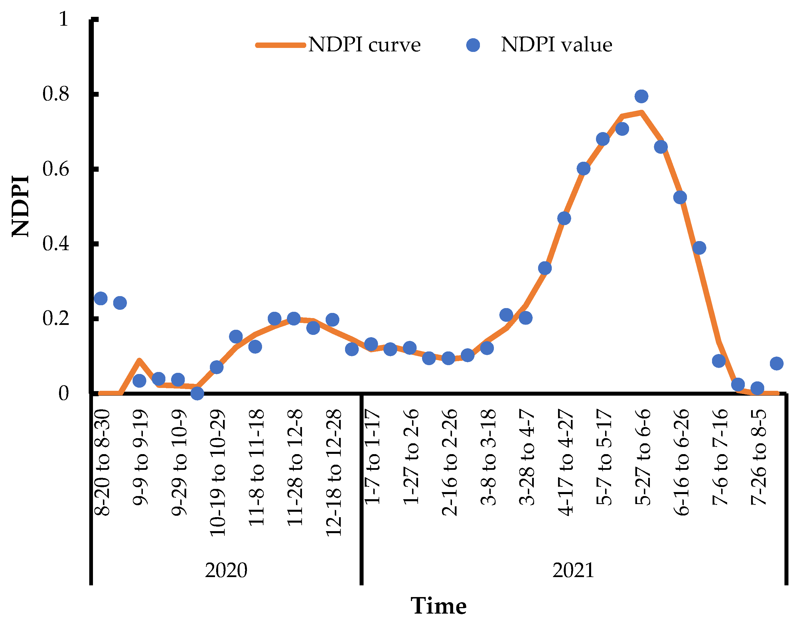
3.1.1. Construction of the Time Series Vegetation Index

This process comprised three parts: quality mosaic cloud removal (Appendix A), NDPI calculation, and S-G filtering.

During vegetation monitoring, the quality mosaic is usually constructed using the normalized difference vegetation index (NDVI) as the quality band [23]. The identification of winter wheat in this study also belongs to the category of vegetation information monitoring. Therefore, NDVI was designated as a quality band for quality mosaic cloud removal in this study. First, the Sentinel-2A/B surface reflectance data were screened from August 2020 to September 2021 as the original image dataset. Then, NDVI was calculated (Equation (7)) for each image and stored in the image dataset as a new band. The original image dataset was then subjected to cloud removal using the quality mosaic algorithm with two adjacent images as the combined unit in chronological order. Finally, a dataset was obtained containing 36 cloud-removed images:

$$\begin{array}{c}\mathrm{NDVI}=\frac{\left(\mathrm{NIR}-\mathrm{R}\right)}{\left(\mathrm{NIR}+\mathrm{R}\right)}\end{array}$$

(7)

where NIR corresponds to B8 from Sentinel-2A/B MSI data and R corresponds to B4 from Sentinel-2A/B MSI data.

Based on the cloud removal image dataset, a new image with 36 NDPI bands, ordered as a chronological time series was created after NDPI calculation (Equation (1)).

In the examination of the images after cloud removal, we found that the images of the 24th, 25th, 30th, and 31st phases were extremely polluted by the cloud. The quality mosaic cloud removal algorithm did not solve this problem, which led to a considerable decrease in the generated NDPI value in the corresponding period. Therefore, we adopted the linear interpolation method to process the above four phases of the images.

Finally, the data were smoothed by the S-G filter and fitted three times at five points (Figure 4). Filtering removed two bands each from the start and end and produced a 32-period high-quality time series vegetation index with a time span of 320 days from 9 September 2020 to 26 July 2021 (

Table 1. Dates corresponding to period number.

Period	3	7	12	17	22	27	34
Start date	2020/9/9	2020/10/19	2020/12/8	2021/1/27	2021/3/18	2021/5/7	2021/6/26
End date	2020/9/19	2020/10/29	2020/12/18	2021/2/6	2021/3/8	2021/5/17	2021/7/26

).

3.1.2. Determination of Samples and Reference Curves

The winter phenological characteristics of winter wheat in the agricultural areas of the plateau valley may not be obvious in the time series performance of the remote sensing images since they are affected by the natural geographical environment and the management methods of the farmland (Figure 5 and Figure 6). To accurately determine the winter wheat samples, vegetation type data from field site surveys and UAV sample data were used for reference sample selection. To explore the wide applicability of the selected characteristic phenophases and their optimized thresholds on the quadrat scale, sample selection, and reference curve construction were conducted on three scales to facilitate their subsequent analysis and application: the individual quadrat, the combined quadrats, and the whole study area (Figure 5).

The orthophoto image data obtained via UAV were georeferenced to the original Sentinel 2A/B image dataset, and the spatial registration of aerial images was realized based on satellite remote sensing images to obtain samples based on the individual scale of the quadrat. Winter and non-winter wheat samples were obtained based on remote sensing satellite images, with the UAV quadrat data and time series vegetation index used as auxiliary references for visual interpretation. Fifty winter wheat truth points were randomly created from the winter wheat sample of quadrat 1 to construct the standard reference sequence, followed by 200 winter wheat truth points and 200 non-winter wheat truth points, which were used for verification. One hundred winter wheat truth points were used from the winter wheat sample of quadrat 2 to construct the standard reference sequence, with 400 winter wheat truth points and 400 non-winter wheat truth points later used for verification. At the same time, the samples of the above two quadrats were combined as truth points at the overall scale of the quadrat.

For the winter wheat, the NDVI value at the seeding stage was small, the NDVI value at the heading stage was large, and the NDVI at the harvesting stage was the smallest. The combination of these three bands can directly reflect the difference between the winter wheat pixels and other types of pixels; therefore, we combined these bands. Based on remote sensing satellite images, point data from the field survey, aerial remote sensing data, NDVI band combined image, and time series NDPI as auxiliary references, 12 winter wheat growing areas were identified. Winter wheat plots and adjacent non-winter wheat plots were visually interpreted, and 13,919 winter wheat sample points and 17,735 non-winter wheat sample points were randomly generated within the plots. Then, 1000 non-winter wheat sample points were randomly generated within the whole study area, and the winter wheat sample points were excluded through artificial judgment. After that, 1200 winter wheat sample points (200 of which were used to construct a standard reference sequence, 1000 for later validation) and 1000 non-winter wheat sample points were extracted from the sample points (

Table 2. The number of truth points selected on different scales.

Study Scale	Winter Wheat Truth Points for Experiment	Winter Wheat Truth Points for Verification	Non-Winter Wheat Truth Points
Quadrat 1	50	200	200
Quadrat 2	100	400	400
Overall quadrat	150	600	600
Overall study area	200	1000	1000

).

The temporal and spatial differences in the winter wheat growth curve were considered to ensure that the reference curve was not overly biased toward winter wheat with good or poor growth in any phenological period. The median NDPI corresponding to the same phenological period as the experimental samples was fitted to obtain the reference curves for winter wheat at three spatial scales (Figure 6).

3.2. Optimization of the Combination of Characteristic Phenological Periods and Their Thresholds

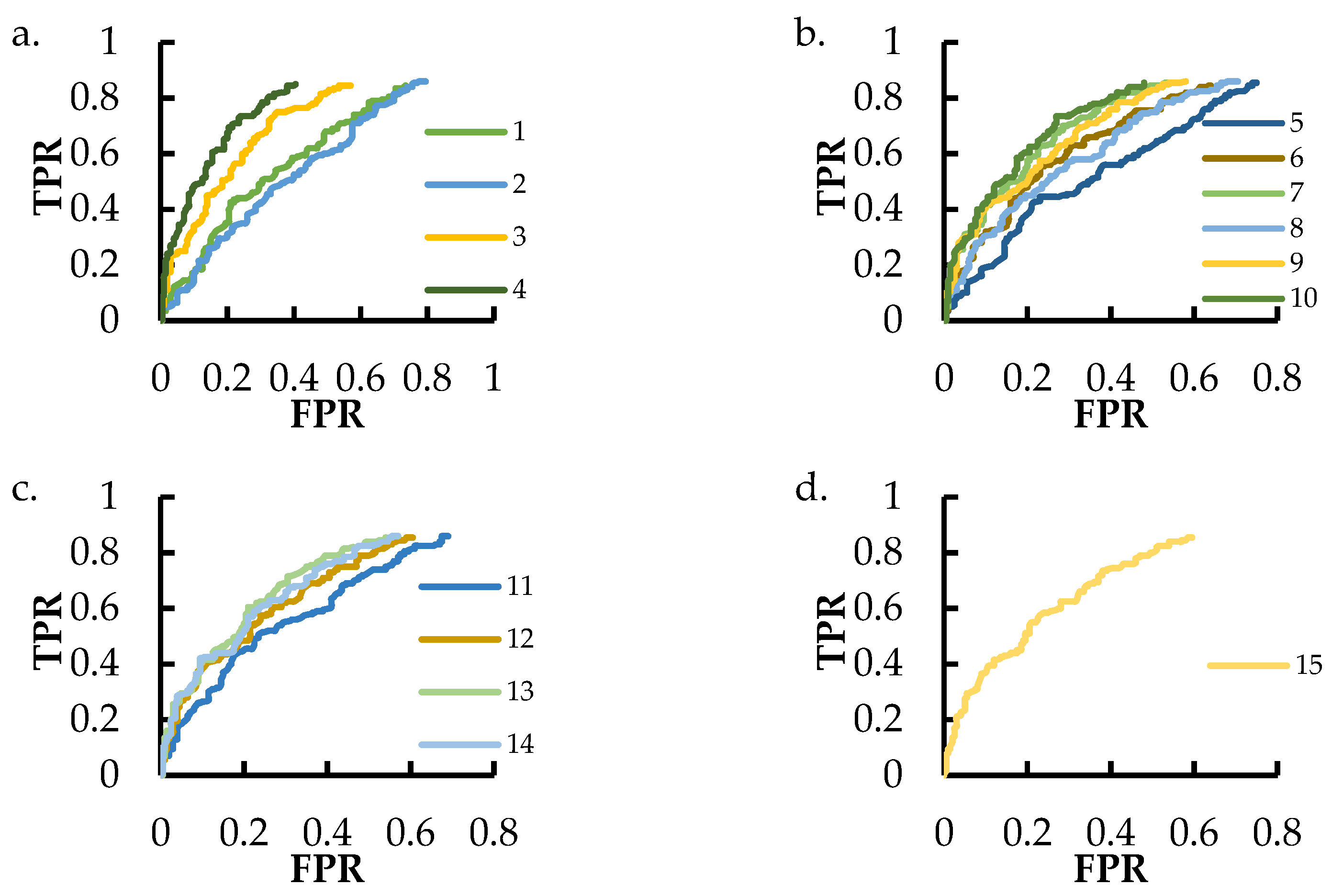
3.2.1. Determination of the Optimal Phenological Period Combination Based on Quadrat Individuals

When using time-series remote sensing images for monitoring, there are often insufficient images for the whole growing season. If a single phenological or double phenological combination with higher accuracy can be selected by comparing all the combinations, winter wheat planting information can be extracted with fewer images. Furthermore, if the selected phenological period is early, it may be possible to realize the early identification of winter wheat. In addition, the jump combination of phenological stages may also help obtain better index characteristics that distinguish winter wheat from other ground objects. Therefore, this study combined and formed four characteristic phenological stages (I, II, III, and IV) representing the combination of the seeding-tillering stage, tillering-overwintering stage, jointing-heading stage, and grouting-harvesting stage, respectively, according to the trend of the NDPI time series curve (Figure 6 and

Table 3. Division of characteristic phenology.

Stage	I	II	III	IV
Periods	4 to 8	10 to 14	21 to 25	26 to 30
Start and end time	2020/9/19 to 2020/10/29	2020/11/18 to 2021/1/7	2021/3/8 to 2021/4/27	2021/4/27 to 2021/6/16

). The extraction experiment of winter wheat was conducted with different combinations of phenological stages at the individual scale of the quadrat.

Preliminary experiments revealed that TPR and ACC did not change with increasing FPR when the threshold was set above 0.26, and the curve was almost parallel to the horizontal axis in the ROC diagram. Therefore, the range of the threshold T was set from 0 to 0.3, and the change step was 0.001. The target NDPI curve and winter wheat reference curve were brought into the DTW model, and the threshold parameters were continuously adjusted. A total of 200 winter wheat sample points and 200 non-winter wheat sample points in quadrat 1 and 400 winter wheat sample points and 400 non-winter wheat sample points in quadrat 2 were used as validation sample points. The ROC plots were drawn according to the experimental results to optimize the optimal threshold of different phenological stage combinations (Figure 7 and Figure 8), and the curve and ACC were used as evaluation indexes to determine the optimal phenological stage combinations (

Table 4. DTW threshold and winter wheat extraction accuracy of the combined time series of different phenological stages in quadrat 1 and quadrat 2.

Sequence Number	Phenological Stage Combinations	Quadrat 1		Quadrat 2
		Optimal Threshold	ACC	Optimal Threshold	ACC
1	I	0.085	0.608	0.084	0.7275
2	II	0.103	0.57	0.075	0.789
3	III	0.182	0.7	0.132	0.905
4	IV	0.181	0.748	0.168	0.916
5	I, II	0.088	0.608	0.071	0.755
6	I, III	0.125	0.663	0.108	0.871
7	I, IV	0.169	0.708	0.126	0.898
8	II, III	0.13	0.635	0.131	0.888
9	II, IV	0.163	0.685	0.135	0.905
10	III, IV	0.181	0.732	0.14	0.908
11	I, II, III	0.114	0.63	0.102	0.866
12	I, II, IV	0.132	0.668	0.121	0.894
13	II, III, IV	0.173	0.705	0.134	0.9
14	I, III, IV	0.177	0.685	0.136	0.905
15	I, II, III, IV	0.175	0.678	0.119	0.898

).

The extraction results of the combined time series of the different phenological periods of the individual quadrat were analyzed under optimal threshold conditions.

The ACC of the time series of phenophase I (60.8%) and phenological stage II (57%) indicated that they showed the worst performance according to quadrat 1 (Table 4 and Figure 7). The ACC of phenological stage III was 70%, and that of phenological stage IV was 74.8%. The extraction result of the combined time series of dual phenology I and II was the worst (ACC = 60.8%), whereas that of the combined time series of dual phenology III and IV was the best (ACC = 73.2%) (Figure 7b and Table 4). The extraction result of the combined time series of triple phenology I, II, and III was the worst (ACC = 63.5%), whereas that of the combined time series of triple phenology II, III, and IV was the best (ACC = 70.5%) (Figure 7c and Table 4). The extraction accuracy of the combined time series of the full phenological stage was 67.8%. A comparison of the extraction accuracy of all combinations of phenological periods showed that the time series of single phenophase IV had the highest extraction accuracy (corresponding threshold T = 0.181, ACC = 74.8%), followed by the combined time series of dual phenology III and IV (T = 0.181, ACC = 73.2%), and the time series of single phenophase III (T = 0.182, ACC = 71.0%).

The regularity of the extraction results of the combined time series of each phenological period of quadrat 2 was similar to that of quadrat 1 (Table 4 and Figure 8). The extraction accuracy of the time series of single phenophases I and II was relatively low (Figure 8a and Table 4), whereas the extraction accuracy of the time series of single phenophases III and IV was relatively high. The extraction result of the combined time series of dual phenology I and II was the worst (ACC = 75.5%) and that of dual phenology III and IV was the best (ACC = 90.8%), compared with the extraction accuracies of the combined time series of dual phenology (Figure 8b and Table 4). The extraction result of the combined time series of triple phenology I, II, and III was the worst (AC = 86.6%), and that of triple phenology I, III, and IV was the best (ACC = 90.5%) (Figure 8c and Table 4). The extraction accuracy of the combined time series of the full phenological stage was 89.8%. The single phenophase IV had the highest extraction accuracy (corresponding DTW threshold T = 0.168, ACC = 91.6%), followed by the combined time series of dual phenology III and IV (corresponding DTW threshold T = 0.140, ACC = 90.8%), and the time series of single phenophase III (corresponding DTW threshold T = 0.132, ACC = 90.5%) among all the combined time series.

The analysis of the extraction results of the combined time series of different phenological periods of the two quadrats (Table 4, Figure 7 and Figure 8) showed that the extraction accuracy of the time series constructed with phenological periods I and II was low, whereas that of phenological periods III and IV was high. The first two phenological stages corresponded to the seeding-tillering stage and the tillering-overwintering stage of winter wheat, respectively. Winter wheat has weak growth at this stage and is affected by the natural environment and farmland management. The difference is insignificant when comparing the NDPI of winter wheat and other features; therefore, the extraction result is poor. Meanwhile, phenological periods III and IV correspond to the jointing-heading stage of winter wheat and the grouting-harvesting stage, respectively. Winter wheat grew and matured rapidly in these two stages, and the corresponding NDPI curve rose, then declined rapidly. This differed significantly from the NDPI of other ground classes; therefore, the extraction results were more accurate.

Further analysis of the spatial distribution of the extraction results (Figure 9) showed that the extraction results of the three optimally combined time series of phenological periods had good spatial distribution, which enabled the relatively accurate extraction of winter wheat, in addition to the partial fragmentation patterns generated by broken farmland. Therefore, based on the results of the two quadrats, the single phenological period Ⅲ (hereinafter referred to as “Plan A”) and the combination of IV (hereinafter referred to as “Plan B”) and dual phenological stages III and IV (hereinafter referred to as “Plan C”) were the best preliminarily selected characteristic phenological stages for the remote sensing extraction of winter wheat in this study area.

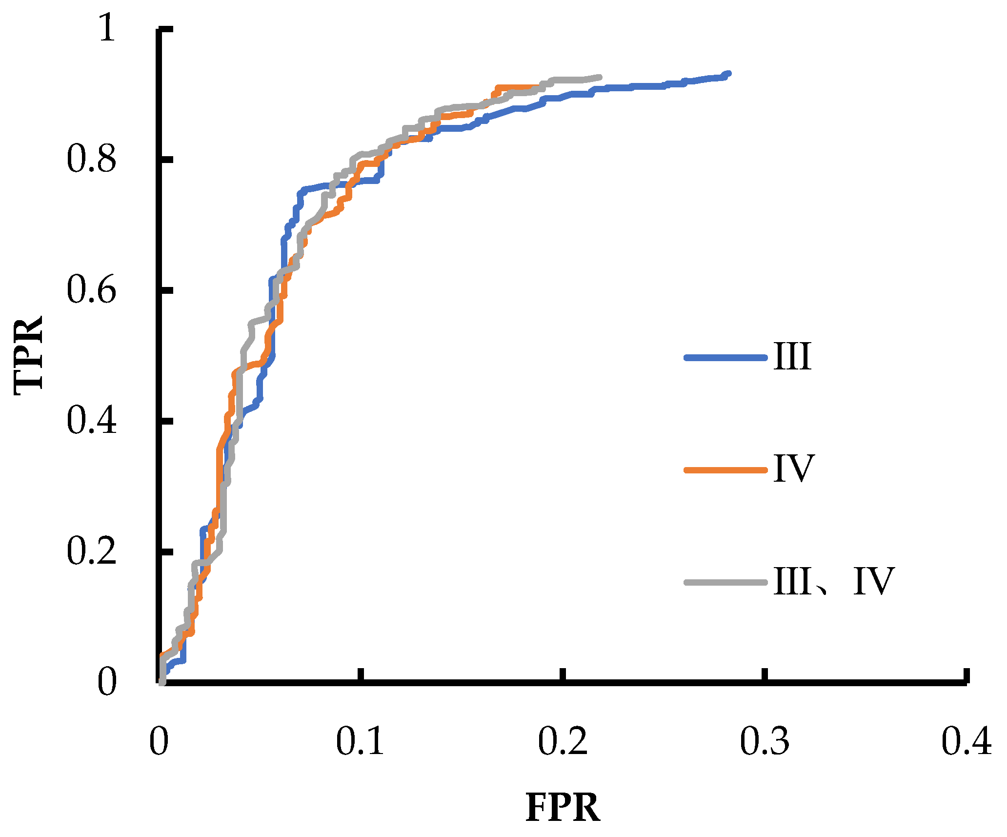
3.2.2. Determination of the Optimal Threshold Based on the Combined Quadrats

The optimal threshold value is variable no matter which combination scheme of the phenological period is used due to the variation in winter wheat growth caused by the difference in geographical location between the two quadrats (Table 4). This brings confusion to the large-scale application of the study. Therefore, it is necessary to comprehensively consider the offset and difference during the same phenology of different regions and consider the two quadrats as a whole to re-optimize the threshold value for the whole region extraction of winter wheat. The specific process is based on the DTW model and the reference curve for all winter wheat in the quadrat. The range of T is 0 to 0.2, and the preliminarily selected time series of Plan A, Plan B, and Plan C were constructed to extract the entire information about wheat planting in the quadrats. Then, 600 winter wheat true value sample points and 600 non-winter wheat sample points were used as test sample points to draw the ROC (Figure 10). The optimal threshold is shown in

Table 5. DTW threshold and winter wheat extraction results of the combined time series of optimal phenological period combinations in the overall quadrat.

Plan	T	TPR	FPR	ACC
Plan A	0.142	0.74	0.167	0.787
Plan B	0.195	0.788	0.178	0.805
Plan C	0.183	0.783	0.195	0.794

.

After the two quadrats were considered as a whole, there was no significant difference in the extraction accuracy of the different combined phenological time series either in the ROC performance or in the accuracy comparison based on the optimal threshold (Table 5, Figure 10), and the extraction results also showed a good performance in determining the spatial distribution (Figure 11). Therefore, the time series of Plan A (T = 0.142) and Plan B (T = 0.195) and the combined time series of Plan C (T = 0.183) had the potential to be informative about winter wheat planting in the whole study area. In practice, Plan A may be the best choice for the identification of early winter wheat. Meanwhile, Plan B or Plan C may be the best choice if we consider the stable and high-precision winter wheat identification in a planting year.

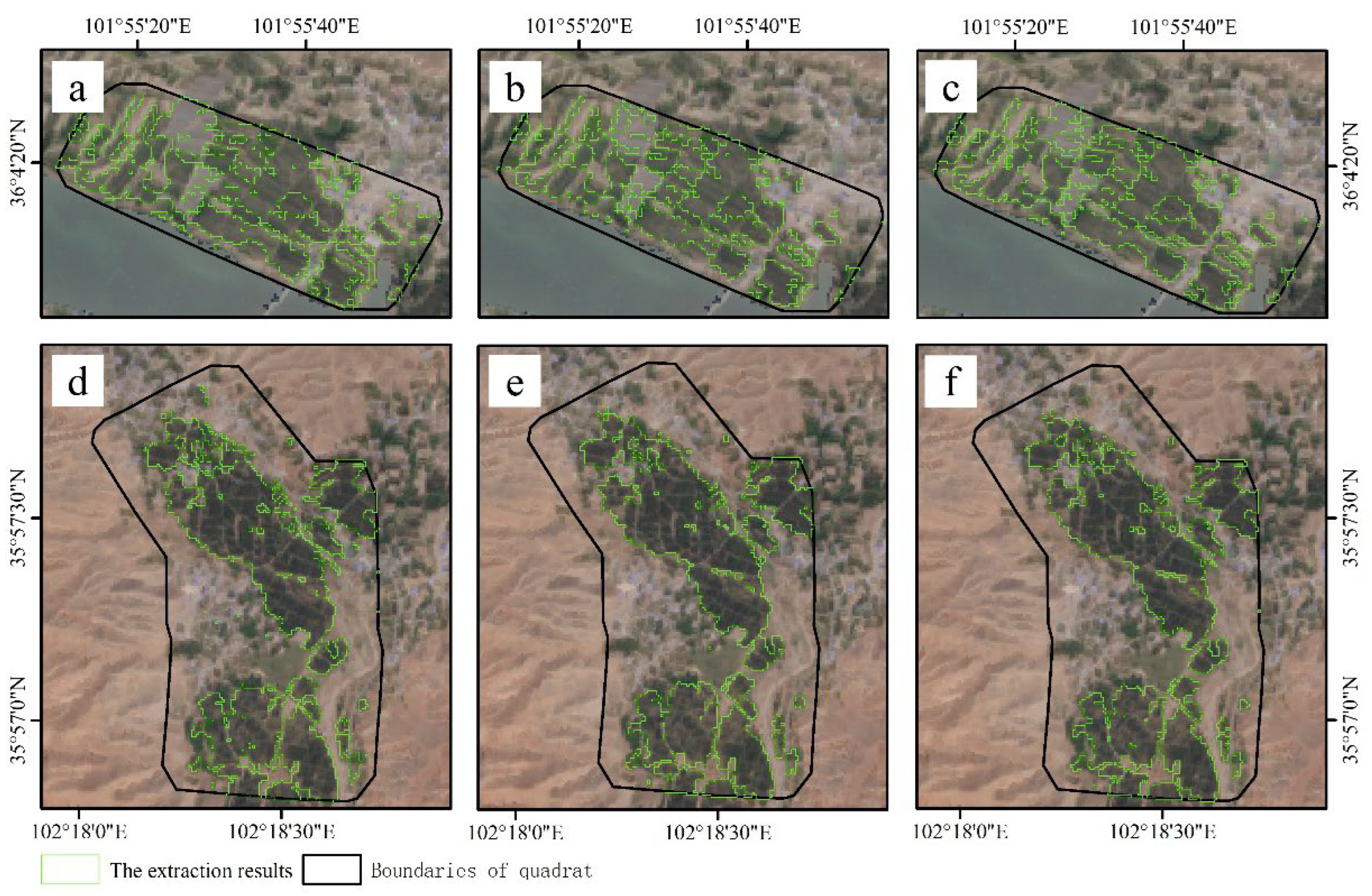
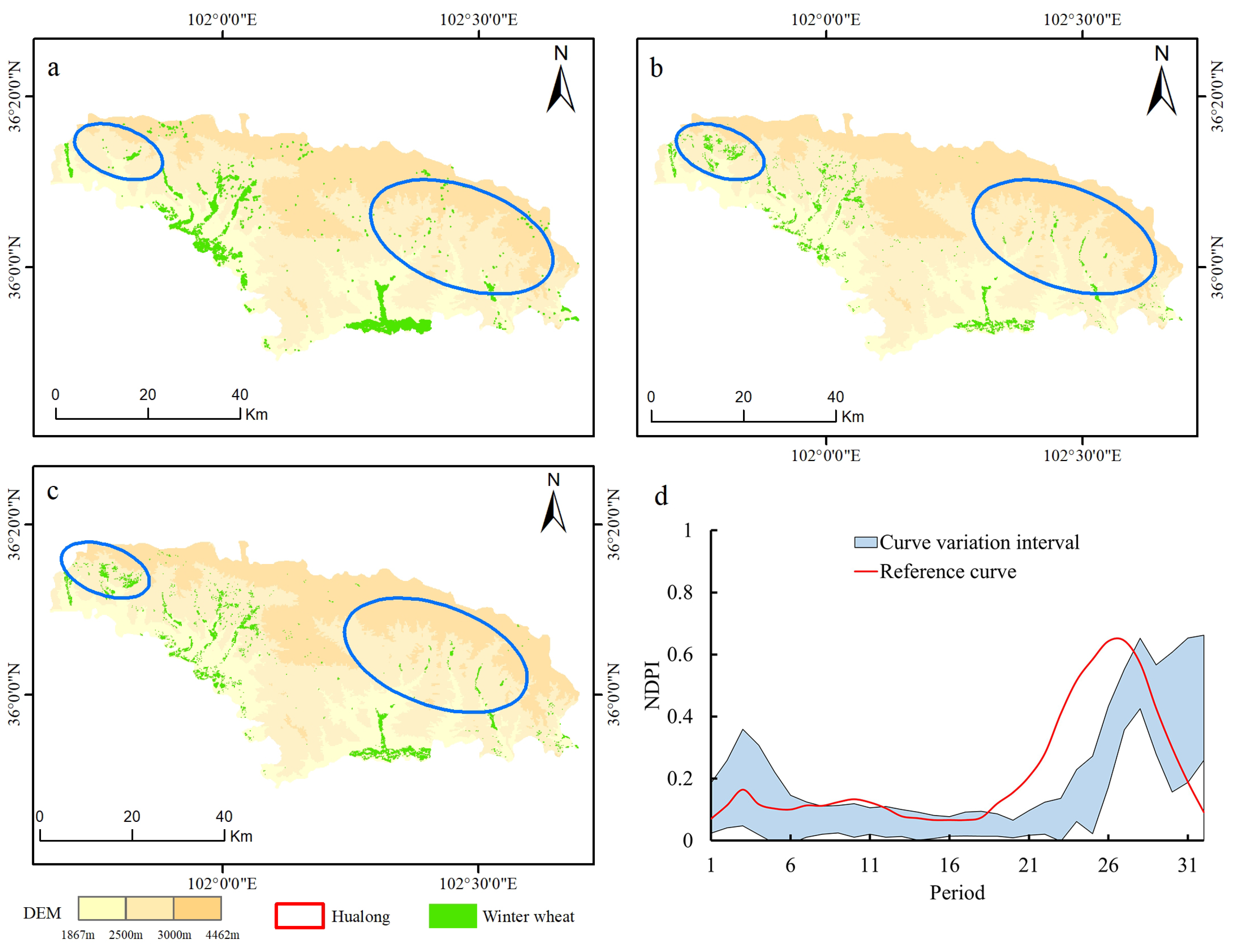
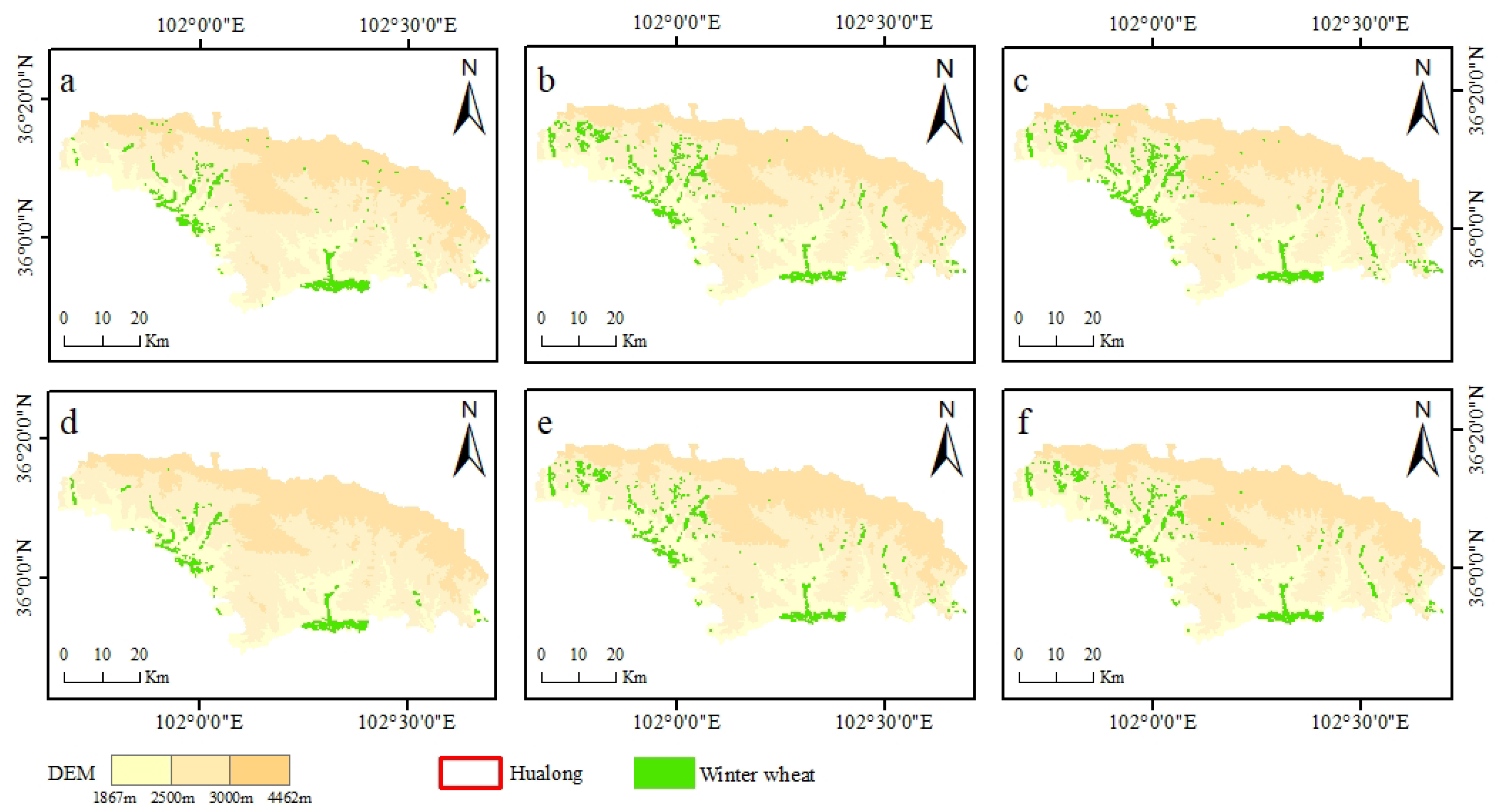
3.3. Extraction of Winter Wheat in the Study Area

The time series of Plan A (T = 0.142), Plan B (T = 0.195), and Plan C (T = 0.183) were used to extract the planting information of winter wheat in the entire study area. This was performed by optimizing the characteristics of the phenological phase combination and its corresponding threshold to further verify the availability of the results based on the DTW model.

There was little difference in FPR and TPR performance among the three combinations of phenological periods according to the ROC accuracy index (

Table 6. DTW threshold and winter wheat extraction results of the combined time series of the optimal phenological period combinations in the study area.

Plan	T	TPR	FPR	ACC	Area
Plan A	0.142	0.828	0.116	0.856	24,130 mu (1689.1 ha)
Plan B	0.195	0.854	0.136	0.859	50,110 mu (3507.7 ha)
Plan C	0.183	0.874	0.138	0.868	33,950 mu (2376.5 ha)

). The performance of Plan C was (TPR, 87.4%; ACC, 86.8%), Plan A was (TPR, 82.8%; ACC, 85.6%), and Plan B was (TPR, 85.4%; ACC, 85.9%). The extraction area of Plan C agreed with the statistical data of approximately 40,000 mu (2800 ha) per year, whereas the time series of Plan A and Plan B indicated a slightly greater bias with the statistical data.

Considering the spatial distribution in Figure 12, the result (Figure 12b) of Plan B is similar to that of Plan C (Figure 12c). However, there are obvious differences between them, and the spatial distribution result corresponded to Plan A (Figure 12a) in several river valleys in the east and west of Hualong. The first two results, corresponding to Plan B and Plan C (Figure 12b,c), showed the winter wheat distribution in the river valley in the east and west of Hualong, whereas the last result, corresponding to Plan A, showed no winter wheat distribution. This study randomly selected sample points in these areas, and the change range was generated and compared with the existing reference The NDPI curve for winter wheat is shown in Figure 12d. The change range of the curve declines around the 28th period but rises again around the 30th period. The pattern is similar to the trend of the standard reference curve; however, the phenological period is relatively delayed by 1 month. In the absence of fieldwork data conditions, this study speculated that the crops grown in these areas were mainly a mixture of spring and winter wheat based on their altitude. That is, because the curves of phenological stage III and IV fitted by DTW are similar, much of the spring wheat might be misclassified as winter wheat in this study area if the early phenological characteristics of the winter wheat are not taken into account. Therefore, in terms of spatial distribution, Plan A is more suitable for the identification of winter wheat, but the extracted results may reveal a smaller area than that of the statistical report.

4. Discussion

4.1. Comparison of NDPI Curve Features of Time Series

The sample median was used to fit the reference curve of the winter wheat. The standard reference curves constructed on different scales were consistent with the overall change trend (a slight increase after the seeding period and a decrease after the tillering period, rapidly increasing after the green-up period, and rapidly decreasing after the heading period) (Figure 6). However, there are still differences among the different characteristic phenophases due to regional differences in water and heat conditions, field management, and other factors caused by growth differences. For example, the two reference curves constructed on the individual scale of the quadrat were different during the whole growth process, and the curve of quadrat 2 was higher than that of quadrat 1 in the growth process after the seeding period. This indicated that the growth status of quadrat 2 was better than that of quadrat 1, which might also be one reason for its higher extraction accuracy than that of quadrat 1. There are also differences between the two curves constructed on the scale of the whole quadrat and the study area, which leads to errors when the optimal threshold is determined based on the whole quadrat and is applied to the entire study area. Therefore, the coupling of reference curves and DTW algorithm thresholds at different scales in practical applications requires further discussion.

Although the current study area was adjacent to that of Huang et al. [23], there was a great difference between the standard growth curves of winter wheat in the two studies (the NDPI curve of the previous study changed significantly between the seeding date and the overwintering stage, whereas the NDPI curve in this study changed insignificantly between the seeding date and the overwintering stage). This resulted in low accuracy when using the single phenological period I or II time series for extraction. It also indicates there may be great differences in crop growth among the different geographical units in the plateau valley. Therefore, it may be more reasonable to construct different models for different geographical units to extract crop planting information.

4.2. Change in the Optimal Threshold

The optimal threshold represents the maximum difference in winter wheat in the study area and in the reference curve. The regional differences in the growth conditions of winter wheat may increase as research strengthens. The winter wheat planting area of quadrat 2 is approximately twice that of quadrat 1, and there may also be greater variation in crop growth; the optimal threshold of quadrat 2 should be larger than that of quadrat 1. However, the opposite is true. Studying the individual scale of the quadrat shows that the optimal thresholds of the individual scale of quadrat 1 and quadrat 2 are 0.182 and 0.132, 0.181 and 0.168, and 0.181 and 0.140 under the extraction of Plan A, Plan B, and Plan C, respectively (Table 4). The optimal threshold for quadrat 1 is greater than that for quadrat 2. Field investigation after the winter wheat overwintering period revealed there was partially unsuccessful overwintering or die-off in the jointing stage of winter wheat in quadrat 1 and its surroundings, whereas there was no such phenomenon in quadrat 2 and its surrounding areas (Figure 13). Therefore, the difference in crop growth is greater in quadrat 1 than that in quadrat 2, which explains why the DTW optimal threshold of quadrat 1 is larger than that of quadrat 2.

The analysis of the reference curve in phenological periods III and IV at the overall scale of the quadrat showed that the optimal thresholds for extraction of Plan A, Plan B, and Plan C were 0.142, 0.195, and 0.183, respectively. This indicates that the dominant effect of the reference curve in the characteristic phenology period IV on the optimal threshold may be stronger than that in the characteristic phenology period III. However, the determination of the optimal threshold of this characteristic may lead to misclassification in areas with uniform growth potential, or it may lead to misclassification in areas with large growth potential differences due to the differences in reference curves; this requires local verification.

4.3. Change in Extraction Accuracy

The extraction accuracy measures the quality of the classifier and the result and reflects the growth of winter wheat. The ACC of quadrat 2 is better than that of quadrat 1 under their respective optimal thresholds. This may be due to the limited spatial resolution of the remote sensing image and the limited recognition of poor growth of winter wheat broken by cultivated land. Quadrat 2 has good and uniform growth, so the overall extraction accuracy is higher than that of quadrat 1. The ACC of the time series extraction results from a single phenological period III decreased compared with quadrat 2 and slightly increased compared with quadrat 1 after considering the two quadrats as a whole. The ACC of the extracted results of Plan C was approximately equal to the mean of the ACC of the two quadrats, which remained at a high level. This shows that the DTW algorithm is relatively limited to the elimination of a small phenological difference.

4.4. Change in the Extracted Area from the Superposition of Cultivated Land Data

This study superimposed the extraction results on high-resolution cultivated land data from existing works. The extraction area of Plan A decreased from 24,130 mu (1689.7 ha) to 20,920 mu (1464.4 ha), and a decrease was observed from 50,110 mu (3507.7 ha) to 43,520 mu (3.46.4 ha) for Plan B; thus, our results were close to the available data (

Table 7. Extraction results with cultivated land support in the study area.

Plan	Area without Cultivated Land Support	Area with Cultivated Land Support
Plan A	2413 mu (1689.7 ha)	2092 mu (1464.4 ha)
Plan B	5011 mu (3507.7 ha)	4352 mu (3046.4 ha)
Plan C	3395 mu (2376.5 ha)	3001 mu (2100.7 ha)

). The extraction area of Plan C decreased from 33,950 mu (2376.5 ha) to 30,010 mu (2100.7 ha). Figure 14 shows that both results, with or without the support of the cultivated data, evaded misclassification to different degrees, and the difference in the extraction results was significantly lowered. This indicates that the extraction results supported by the cultivated land data may be more reliable than those without; however, the missing score error within the cultivated land needs further investigation.

4.5. Early Identification of Winter Wheat with Cultivated Land Support

The results of the first two phenological periods (phenophases I and II) were superposed on the reference cultivated land data to improve the early identification accuracy of winter wheat. The extraction accuracy of the time series of single phenophases I and III was improved on the individual quadrat scale, and the highest value was observed in quadrat 2 (83.0%) (

Table 8. Extraction results from cultivated land support of the first two phenological periods.

Quadrat	Quadrat 1	Quadrat 1	Quadrat 2	Quadrat 2	Overall Quadrat	Overall Quadrat
Phenological period	I	II	I	II	I	II
Optimal threshold	0.085	0.103	0.084	0.075	0.113	0.102
ACC without cultivated land support	0.608	0.570	0.728	0.789	0.598	0.60
ACC with cultivated land support	0.640	0.625	0.830	0.819	0.723	0.695

). A superposition analysis was also performed at the overall quadrat scale, as the results at the individual scale of the quadrat may not be representative and universal. The extraction accuracy of the overall scale of the quadrat (72.3%) is higher than that of quadrat 1 but lower than that of quadrat 2. The phenological characteristics of winter wheat in this study area were not obvious before the overwintering stage; however, early identification of winter wheat still has potential under cultivated land support.

5. Conclusions

This study explored the optimization of the characteristic phenological period in the extraction process of winter wheat based on time series remote sensing image data and the DTW model in the agricultural area of the plateau valley. Using GEE and the NDPI time series curve of the winter wheat growing season in Hualong, China, in 2020–2021, this comparative study analyzed winter wheat based on the NDPI time series of different phenological periods. The main conclusions are: (1) NDPI corresponding to the jointing-heading stage, the grouting-harvesting stage, and jointing-harvesting stage with DTW could be effectively utilized to identify winter wheat regardless of the spatial scale whether in a single quadrat, a combination of two quadrats, or the entire study area. (2) NDPI corresponding to the jointing-heading stage (Plan A, corresponding to the DTW threshold T = 0.158) may be the optimal selection if we consider the rationality of spatial distribution. Furthermore, the area may be statistically small if we consider the statistical report data. Hence, the NDPI corresponding to grouting-harvesting stage (Plan B, corresponding to the DTW threshold T = 0.195) may be the optimal selection under cultivated land support. (3) The early identification of winter wheat is possible based on the phenological characteristics of the wheat before the overwintering stage and cultivating of the land.

References

1. Guo, X.; Wang, N.; Zhang, L.; Guo, Y.; Chu, X.; Feng, H. Extraction of winter wheat information based on time-series NDVl in Guanzhong area. J. Agric. Res. Arid Areas 2020, 38, 275–280. (In Chinese) [Google Scholar]
2. Jiang, Y.; Chen, B.; Huang, Y.; Cui, J.; Guo, Y. Crop planting area extraction based on Google Earth Engine and NDVI time series difference Index. J. Geo-Inf. Sci. 2021, 23, 938–947. (In Chinese) [Google Scholar]
3. Hu, Q.; Wu, W.; Song, Q.; Yu, Q.; Yang, P.; Tang, H. Recent progresses in research of crop patterns mapping by using remote sensing. J. Sci. Agric. Sin. 2015, 48, 1900–1914. (In Chinese) [Google Scholar]
4. Zhang, J.; Zhao, G.; Hong, Y.; Sun, Z.; Duan, Y. Spatial extraction of winter wheat in Hebei in growing season using pixel-wise phenological curve. J. Trans. Chin. Soc. Agric. Eng. 2020, 36, 193–200. (In Chinese) [Google Scholar]
5. Conese, C.; Maselli, F. Use of multitemporal information to improve classification performance of TM scenes in complex terrain. J. ISPRS J. Photogramm. Remote Sens. 1991, 46, 187–197. [Google Scholar] [CrossRef]
6. Li, R.; Li, G.; Lu, X.; Zhang, X.; Yu, H. An improved method of winter wheat remote sensing recognition based on time series. J. Sci. Surv. Mapp. 2022, 47, 73–79+110. (In Chinese) [Google Scholar]
7. Pan, Y.; Li, L.; Zhang, J.; Liang, S.; Hou, D. Crop area estimation based on MODIS-EVI time series according to distinct characteristics of key phenology phases: A case study of winter wheat area estimation in small-scale area. J. Remote Sens. 2011, 15, 578–594. (In Chinese) [Google Scholar]
8. Chen, J.; Tian, Q. Vegetation classification based on high-resolution satellite image. J. Remote Sens. 2007, 11, 221–227. [Google Scholar]
9. Zhao, Y.; Wang, X.; Hou, X. Spatio-temporal characteristics of key phenology of winter wheat in Shandong Province from 2003 to 2019. Acta Ecol. Sin. 2021, 41, 7785–7795. [Google Scholar]
10. Luo, Y.; Zhang, C.; Zhang, L. Simulation of spatial and temporal variability of winter wheat phenology and analysis of its climate drivers based on an improved pDSSAT model. Sci. Sin. (Terrae) 2022, 52, 126–143. [Google Scholar]
11. Liu, Y.; Chen, Q.; Ge, Q. Spatiotemporal differentiation of changes in wheat phenology in China under climate change from 1981 to 2010. Sci. Sin. (Terrae) 2018, 48, 888–898. (In Chinese) [Google Scholar] [CrossRef]
12. Wang, H.; Gong, Y.; Liu, W.; Li, Z.; Zhang, S. Study on spatial-temporal multiscale adaptive method of gesture recognition. Comput. Sci. 2017, 44, 287–291. [Google Scholar]
13. Bankó, Z.; Abonyi, J. Correlation based dynamic time warping of multivariate time series. Expert Syst. Appl. 2012, 17, 12814–12823. [Google Scholar] [CrossRef]
14. Petitjean, F.; Inglada, J.; Gançarski, P. Satellite image time series analysis under time warping. IEEE Trans. Geosci. Remote Sens. 2012, 50, 3081–3095. [Google Scholar] [CrossRef]
15. Guan, X.; Huang, C.; Liu, G.; Xu, Z.; Liu, Q. Extraction of paddy rice area using a DTW distance based similarity measure. Resour. Sci. 2014, 36, 267–272. [Google Scholar]
16. Sakoe, H.; Chiba, S. Dynamic programming algorithm optimization for spoken word recognition. IEEE Trans. Acoust. Speech Signal Process. 1978, 26, 43–49. [Google Scholar] [CrossRef] [Green Version]
17. Hamooni, H.; Mueen, A.; Neel, A. Phoneme sequence recognition via DTW-based classification. Knowl. Inf. Syst. 2016, 48, 253–275. [Google Scholar] [CrossRef]
18. Maus, V.; Câmara, G.; Appel, M.; Pebesma, E. dtwsat: Time-weighted dynamic time warping for satellite image time series analysis in R. J. Stat. Softw. 2019, 88, 1–31. [Google Scholar] [CrossRef] [Green Version]
19. Duan, J.; Xu, Y.; Sun, X.-Y. Spatial patterns and their changes of grain production, grain consumption and grain security in the Tibetan Plateau. J. Nat. Res. 2019, 34, 673–688. (In Chinese) [Google Scholar] [CrossRef]
20. Liu, M.; Wang, B.; Zhong, J. Population-Economic-Grain Regional Difference and Spatial Pattern of Qinghai Province in the Past 30 Years. Northwest Popul. J. 2021, 42, 113–124. (In Chinese) [Google Scholar]
21. Chen, Y.; Zhou, Q.; Chen, Q.; Mao, X.; Liu, F. The response of grain crops in Hehuang Valley to the climate change nearly 20 years. Agric. Res. Arid Areas 2018, 36, 223–229, 241. [Google Scholar]
22. Chen, R.; Zhou, Q.; Liu, F.; Zhang, Y.; Chen, Q.; Chen, Y. Contribution of climate change to food yield in Yellow River-Huangshui River Valley. Hubei Agric. Sci. 2018, 57, 114–119. (In Chinese) [Google Scholar]
23. Huang, F.; Xia, X.; Huang, Y.; Lv, S.; Chen, Q.; Pan, Y.; Zhu, X. Comparison of winter wheat extraction methods based on different time series of vegetation indices in the Northeastern margin of the Qinghai–Tibet Plateau: A case study of Minhe, China. Remote Sens. 2022, 14, 343. [Google Scholar] [CrossRef]
24. Gu, X.; Song, G.; Han, J.; Xu, C.; Pan, Y. Monitoring of growth changes of winter wheat based on change vector analysis. Trans. CSAE 2008, 24, 159–165+1. (In Chinese) [Google Scholar]
25. Singh, R.; Semwal, D.P.; Rai, A.; Chhikara, R.S. Small area estimation of crop yield using remote sensing satellite data. Int. J. Remote Sens. 2002, 23, 49–56. [Google Scholar] [CrossRef]
26. Hualong County People’s Government Official Website. Available online: http://www.hualongxian.gov.cn/html/1143/294809.html (accessed on 2 May 2021). (In Chinese)
27. Jin, X.; Ma, J. Discussion on the conditions and control technology of yellow dwarf disease of wheat in Hualong County. Qinghai Agro-Technol. Ext. 1999, 4, 60. (In Chinese) [Google Scholar]
28. Hualong County becomes one of the largest winter wheat production bases in the province. Cereals Oils Process. 2009, 8, 19. (In Chinese)
29. The Harvested Crop Area in Hualong Reaches 166,000 mu. Available online: http://www.moa.gov.cn/xw/qg/201909/t20190927_6329164.htm (accessed on 15 December 2022). (In Chinese)
30. Hualong County Had a Good Harvest of Winter Wheat. Available online: http://www.qinghai.gov.cn/zwgk/system/2020/07/14/010362574.shtml (accessed on 15 December 2022). (In Chinese)
31. Hualong: Thousands of Hectares of Winter Wheat Green Yellow River Valley. Available online: https://epaper.tibet3.com/qhrb/html/202210/24/content_114965.html (accessed on 15 December 2022). (In Chinese).
32. Winter Wheat is Growing Well in Hualong County. Available online: http://www.dbcsq.com/dbcsq/202210/190838.html (accessed on 15 December 2022). (In Chinese).
33. Tian, Y.; Jia, M.; Wang, Z.; Mao, D.; Du, B.; Wang, C. Monitoring invasion process of Spartina alterniflora by seasonal Sentinel-2 imagery and an object-based random forest classification. Remote Sens. 2020, 12, 1383. [Google Scholar] [CrossRef]
34. Song, H.; Lei, H.; Shang, M. Crop classification based on Sentinel 2A/B time series data in Heilonggang river basin. Jiangsu J. Agric. Sci. 2021, 37, 83–92. [Google Scholar]
35. The National Catalogue Service for Geographic Information. Available online: https://www.webmap.cn/main.do?method=index (accessed on 2 May 2021). (In Chinese).
36. Fan, D.; Zhao, X.; Zhu, W.; Zheng, Z. Review of influencing factors of accuracy of plant phenology monitoring based on remote sensing data. Prog. Geogr. 2016, 35, 304–319. (In Chinese) [Google Scholar]
37. Luo, Y.; Xu, J.; Yue, W. Research on vegetation indices based on the remote sensing images. Ecol. Sci. 2005, 24, 75–79. (In Chinese) [Google Scholar]
38. Dong, Q.; Chen, X.; Chen, J.; Zhang, C.; Liu, L.; Cao, X.; Zang, Y.; Zhu, X.; Cui, X. Mapping winter wheat in North China using Sentinel 2A/B data: A method based on phenology-time weighted dynamic time warping. Remote Sens. 2020, 12, 1274. [Google Scholar] [CrossRef] [Green Version]
39. Shi, X.; Ming, Y.; Liu, C.; Qu, Y.; Sui, S. Analysis on the application of time series image in extraction of winter wheat planting area. Radio Eng. 2021, 51, 1567–1576. (In Chinese) [Google Scholar]
40. Li, F.; Ren, J.; Wu, S.; Zhang, N.; Zhao, H. Effects of NDVI time series similarity on the mapping accuracy controlled by the total planting area of winter wheat. Trans. CSAE 2021, 37, 127–139. (In Chinese) [Google Scholar]
41. Liang, S.; Shi, P.; Xing, Q. A Comparison Between the Algorithms for Removing Cloud Pixel from MODIS NDVI Time Series Data. Remote Sens. Nat. Resour. 2011, 1, 33–36. (In Chinese) [Google Scholar]
42. Carreiras, J.M.B.; Pereira, J.M.C.; Shimabukuro, Y.E.; Stroppiana, D. Evaluation of compositing algorithms over the Brazilian Amazon using SPOT-4 VEGETATION data. Int. J. Remote Sens. 2003, 24, 3427–3440. [Google Scholar] [CrossRef]
43. Viovy, N.; Arino, O.; Belward, A.S. The Best Index Slope Extraction (BISE): A method for reducing noise in NDVI time-series. Int. J. Remote Sens. 1992, 13, 1585–1590. [Google Scholar] [CrossRef]
44. Lovell, J.L.; Graetz, R.D. Filtering pathfinder AVHRR land NDVI data for Australia. Int. J. Remote Sens. 2001, 22, 2649–2654. [Google Scholar] [CrossRef]
45. Savitzky, A.; Golay, M.J.E. Smoothing and differentiation of data by simplified least squares procedures. Anal. Chem. 1964, 36, 1627–1639. [Google Scholar] [CrossRef]
46. Li, H.-Y.; Jia, Y.-W.; Ma, M.-G. Reconstruction of temporal NDVI dataset: Evaluation and case study. Remote Sens. Technol. Appl. 2009, 24, 596–602. (In Chinese) [Google Scholar]
47. Chen, J.; Jönsson, P.; Tamura, M.; Gu, Z.; Matsushita, B.; Eklundh, L. A simple method for reconstructing a high-quality NDVI time-series data set based on the Savitzky–Golay filter. Remote Sens. Environ. 2004, 91, 332–344. [Google Scholar] [CrossRef]
48. Zhao, H.; Zhou, Y.; Pei, T.; Chen, Y.; Xie, B. Spatiotemporal analyses of vegetation coverage variation and its responses to slope in Middle East of Gansu Province. Remote Sens. Inf. 2019, 34, 133–139. (In Chinese) [Google Scholar]
49. Dong, J.; Fu, Y.; Wang, J.; Tian, H.; Fu, S.; Niu, Z.; Han, W.; Zheng, Y.; Huang, J.; Yuan, W. Early-season mapping of winter wheat in China based on Landsat and Sentinel images. Earth Syst. Sci. Data 2020, 12, 3081–3095. [Google Scholar] [CrossRef]
50. Zhang, Y. Query tree feature extraction based on data mining for detecting SQL injection attack. Appl. Electron. Tech. 2016, 42, 90–94. [Google Scholar]
51. Zhu, W.; Zeng, N.; Wang, N. Sensitivity, specificity, accuracy, associated confidence interval and ROC analysis with practical SAS implementations. In Proceedings of the NESUG 2010: Health Care and Life Sciences, Baltimore, MA, USA, 14–17 November 2010. [Google Scholar]
Figure 1. Study area. (a) Location of the Hehuang Valley; (b) Location of Hualong; (c) Hualong digital elevation model.
Remotesensing 15 00028 g001
Figure 2. (a) Location of two quadrats; (b) Quadrat 1; (c) Quadrat 2.
Remotesensing 15 00028 g002
Figure 3. Dynamic time warping (DTW) algorithm.
Remotesensing 15 00028 g003
Figure 4. Savitzky–Golay (S-G) filtering effects.
Remotesensing 15 00028 g004
Figure 5. Sample selection. (a) Location of three samples in the study area; (b1,c1,d1) Remote-sensing image of Sentinel 2A/B; (b2,c2) Quadrat image; (d2) NDVI (normalized difference vegetation index) combination image; (b3,c3,d3) Sample points corresponding to NDPI curves.
Remotesensing 15 00028 g005
Figure 6. Winter wheat reference curves on different scales and phenological periods of winter wheat. a: Total quadrats; b: Quadrat 1; c: Quadrat 2; d: Study area.
Remotesensing 15 00028 g006
Figure 7. Extraction results of quadrat 1 combination at different phenological stages. (a) Single phenophase; (b) Combined time series of dual phenology; (c) Combined time series of triple phenology; (d) Full phenological stage with 1–15 corresponding to the combination numbers of different phenological stages in Table 4. FPR—false positive rate; TPR—true positive rate.
Remotesensing 15 00028 g007
Figure 8. Extraction results of quadrat 2 combination at different phenological stages. (a) Single phenophase; (b) Combined time series of dual phenology; (c) Combined time series of triple phenology; (d) Full phenological stage with 1–15 corresponding to the combination numbers of different phenological stages in Table 4.
Remotesensing 15 00028 g008
Figure 9. Winter wheat extraction results under optimal thresholds of the two quadrats. (a) Extraction results of quadrat 1 in Plan A; (b) Extraction results of quadrat 1 in Plan B; (c) Extraction results of quadrat 1 in Plan C; (d) Extraction results of quadrat 2 in Plan A; (e) Extraction results of quadrat 2 in Plan B; (f) Extraction results of quadrat 2 in Plan C.
Remotesensing 15 00028 g009
Figure 10. Extraction results of three combinations of phenological periods.
Remotesensing 15 00028 g010
Figure 11. Results of winter wheat extraction under optimal thresholds of the two quadrats. (a,d) Extraction results of the overall quadrat in Plan A. (b,e) Extraction results of the overall quadrat in Plan B. (c,f) Extraction results of the overall quadrat in the Plan C.
Remotesensing 15 00028 g011
Figure 12. Extraction result of the study area. (a) Extraction results of Plan A; (b) Extraction results of Plan B; (c) Extraction results of Plan C; (d) Comparison of phenological periods.
Remotesensing 15 00028 g012
Figure 13. Winter wheat in quadrat 1 and its nearby areas which died of disease. (a) Winter wheat die-off in the jointing stage; (b) Some of winter wheat failed to overwinter. (picture taken on 2 May 2021).
Remotesensing 15 00028 g013
Figure 14. Extraction results with cultivated land support. (a) Extraction results in Plan A; (b) Extraction results in Plan B; (c) Extraction results in Plan C; (d) Extraction results in Plan A with cultivated land support; (e) Extraction results in Plan B with cultivated land support; (f) Extraction results in Plan C with cultivated land support.
Remotesensing 15 00028 g014