Forest Area and Structural Variable Estimation in Boreal Forest Using Suomi NPP VIIRS Data and a Sample from VHR Imagery

Abstract

Our objective was to develop a method for the assessment of forest area and structural variables for cases in which the availability of representative ground reference data is poor and these data are not collected from the whole area of interest. We implemented two independent approaches to the estimation of the forest variables of a European boreal forest: (i) the computation of wall-to-wall estimates using moderate- to low-resolution VIIRS imagery from the Suomi NPP mission; and (ii) the visual interpretation of plots of samples from very high resolution (VHR) satellite data obtained via a two-stage design. Our focus was on the statistical comparison of forest resources at a country or larger level. The study area was boreal forest ranging from Norway to the Ural Mountains in Russia. We computed a seamless mosaic from 111 VIIRS images. From the mosaic, we computed predictions for the forest area, growing stock volume, height of the dominating tree layer, proportion of conifers and broadleaved trees, site fertility class, and leaf area index. The reference data for the VIIRS imagery were national forest inventory (NFI)-based raster maps from Finland. The first stage sample of VHR data included 42 images; of these, a second stage sample of 2690 plots was visually interpreted for the same variables. The forest area prediction from VIIRS for the whole study area was 1.2% higher than the VHR-based result. All other structural variable predictions using VIIRS fitted within the 95% confidence intervals computed from the VHR sample except for estimates of the main tree species groups, which were outside the limits. A comparison of VIIRS-based forest area estimates using Finnish and Swedish NFI data indicated overestimations of 10.0% points and 4.6% points, whereas the total growing stock volumes were overestimated by 8% and underestimated by 3.4%, respectively. The correlation coefficients between the VIIRS and VHR image predictions at the 42 VHR image locations varied from 0.70 to 0.85. The VIIRS maps strongly averaged the local predictions due to their coarse spatial resolutions. Based on our findings, the approach using two independent estimations yielded similar figures for the central forest variables for the European boreal forest. A model computed using reference data from a small part of the area of interest can provide satisfactory predictions for a much larger area with a similar biome. Therefore, our concept is applicable to the estimation and overall mapping of a forest area and central structural variables at regional to national levels.

1. Introduction

Concern for the sustainability of raw material supply, as well as ecological and carbon cycle issues, requires the availability of information about forest area, biomass, species, and other forest resources beyond the borders of individual countries [1,2,3]. Satellite imagery, which is a globally available source of information, has been used for mapping and monitoring forest cover as an explicit topic of interest or as part of land cover mapping [4,5]. The principal motivation in satellite-image-based surveys has been to monitor the forest area, biomass and, to a lesser extent, the main species.

Forest area is the principal variable in forest inventories and land cover mapping. The national forest inventories (NFIs) provide statistical information about forest area, structural forest variables, and other forest ecosystem characteristics, such as site fertility. The NFIs are usually based on the statistical sampling of ground plots, potentially supported by remotely sensed image data. The sampling-based national forest inventories have been conducted for more than 100 years in few countries, such as Finland [6]. They are, however, expensive to conduct; consequently, the information may not be up to date. The pure sampling-based inventories do not usually produce thematic wall-to-wall maps. However, in some countries, such as the United States, Finland, and Sweden, satellite imagery and NFI ground plots have been and are still being used to compute thematic map layers of forest variables [7,8].

The NFI plot data are country-specific, and their access may be restricted, particularly when permanent sample plots, which are becoming more common, are used. Other means of deriving information about forests should be developed for surveys of wider areas.

The perspective of most forest-related projects that have utilized satellite images has been to make maps of the forest cover instead of providing actual forest inventory data. The map spatial resolution has ranged from 1 × 1 km² to 10 × 10 m² [4,5,9,10]. Most of the maps have used optical data, but radar-based global forest/non-forest maps have also been published [11,12]. Regional mapping has been reported, e.g., in [13,14]. Forest extent predictions have varied greatly between global and continental maps made by different research teams. The reasons for these differences are variable forest definitions, satellite data sources, spatial resolutions, and image analysis methods which make their comparison difficult [15]. For example, in a study comparing eight land cover classifications, the coefficient of determination for the percentage of forest cover with the training data from Google Earth varied from 0.53 to 0.81. The individual maps were combined to compute a “best guess” map using visually interpreted samples from Google Earth [16]. Official country statistics and sampled tracks of light detection and ranging (Lidar) have also been used as calibrating data in mapping [17,18].

Groups of main tree species have been predicted from satellite data at beyond-country extents, mainly in the context of general land cover mapping. A sophisticated approach using a Landsat data cube, lower-resolution satellite imagery, and ensemble learning was used to compute global land cover maps. These maps included three classes for species: broadleaf, needle-leaf, and mixed forest. The average percentage of correctly classified land cover classes of the 25 classes was 80.6% at the global level. Relatively high uncertainties were reported for boreal tundra and boreal mountain systems [9]. In a boreal forest study in Europe, cross-validation was used to test the uncertainty for three species groups: coniferous, broadleaved trees, and mixed forest. The correct classification for these groups varied between 60 and 70% [19]. The uncertainty was lower than with the Coordination of Information on the Environment (CORINE) maps [20].

A growing stock volume map of the Nordic countries and European Russia was computed by modeling the volume using ground plots and Landsat Thematic Mapper data from Finland and extrapolating the model for cross-calibrated NOAA AVHRR imagery. Using data obtained from the national forest inventory, the models were assessed using growing stock volume data from 20 forest districts in Finland. The best model used red band only and showed a correlation of 0.98 with the forestry district volumes. No data for assessing uncertainty were available for Russia. The models did not separate the forest from the non-forest area well, and they overestimated the volumes close to the forest line regions [21]. A similar mapping project was conducted using Sentinel-2 data at a resolution of 10 m; this project had the same challenges with respect to uncertainty assessment [22].

Space-borne lidar, the Geoscience Laser Altimeter System (GLAS), was used to compute two pan-tropical biomass maps by extrapolating the strip-wise Lidar data using optical and microwave imagery. The maps were produced at resolutions of 1 km and approximately 0.5 km. The biomass was estimated through the relationship between the forest height, initially predicted from the GLAS data, and biomass [23,24]. The maps differed substantially despite similar approaches to data analysis. A fused map was computed from these two sources using 1 km calibration plots which were based on high-resolution biomass maps [25].

Projects such as those using GLAS data have been implemented through the use of Global Ecosystem Dynamics Investigation (GEDI) lidar data. The assessment was based on a forest height estimation. The level of uncertainty varied between regions and vegetation types [26,27]; however, saturation at the high levels of biomass typical for passive optical data [28] was not clear using GEDI observations. The GEDI was an experimental mission onboard the International Space Station.

A global biomass map was computed using two space-borne radar sensors: the Phased Array type L-band Synthetic Aperture Radar (PALSAR) instrument onboard the Advanced Land Observing Satellite (ALOS) satellite and the Advanced Synthetic Aperture Radar (ASAR) instrument operating at the C-band onboard the Environmental Satellite (Envisat). The SAR-based estimate started to saturate at approximately 200 metric tons/ha, leading to an underestimation of the biomass. The study used a forest area map from the Climate Change Initiative (CCI) to separate forest areas from other land cover types; however, this led to higher estimates for the total biomass compared to the Forest Resources Assessment (FRA) of the Food and Agriculture Organization (FAO) of the United Nations [29].

The literature review revealed that an objective assessment of the forest area and forest attribute maps from satellites is difficult due to the varying definitions of forest, miscellaneous and poorly representative reference data for uncertainty assessments, varying study area sizes, and varying spatial resolutions of the imagery. Field reference data from national forest inventories are available from a few countries only. The best approach to compiling forest maps with as high a reliability as possible has been to combine different maps in a justified way. However, in these cases, the true reliability of a map also remains unclear.

In this study, we developed a concept aimed at reducing the uncertainty that was common in earlier projects estimating forest variables over large areas. Such a concept is not restricted to any specific type of satellite imagery that is used for wall-to-wall mapping and variable prediction. We compared two approaches for estimating the forest area and forest structural variables over the boreal forest of Fennoscandia and Western Russia: (1) model-based estimates based on maps developed from Visible Infrared Imaging Radiometer Suite (VIIRS) data from the Suomi National Polar-Orbiting Operational Environmental Satellite System Preparatory Project (Suomi NPP) satellite (later VIIRS), and (2) sample-based estimates using a sample from very high resolution (VHR) images. Reference data for the VIIRS-based model were available from Finland only. Thus, the key underlying question of this work is whether a model-based approach that extrapolates over a large area (outside Finland) is comparable to an independent, sample-based approach that covers the entire population.

The variables estimated from the VIIRS data were the forest area, growing stock volume, the height of the dominating tree layer (Lorey’s height), the proportion of conifers and broadleaved trees from volume, the site fertility class, and the leaf area index (LAI). The site fertility classification followed the Finnish forest type system, which is based on the species of undergrowth vegetation [30]. The concept of forest was defined as land covered by trees with a tree height of more than 5 m at a mature stage and a crown closure of at least 10%. Forests found in built-up areas were also included in this class when they fulfilled the conditions.

The same variables as those from the moderate-resolution data were assessed from the VHR data except that within the conifers, the proportions of Scots pine and Norway spruce were additionally separated. Other conifer species and other broadleaved trees were grouped into two categories, but their proportions were minor. The LAI was not evaluated from VHR imagery but from the crown cover percentage instead.

We hypothesized that the two independent approaches would aid in understanding the uncertainties that occur when the forest cover and attribute estimates are based on the exclusive use of Earth observation data or on the use of reference data that are only available for a fraction of the area of interest. If the VIIRS-imagery-based estimates fit within the 95% confidence intervals of the variables that were computed from the VHR image sample, the derived information for the forest variables could be considered realistic. Unlike some earlier studies [31,32], we did not use the VHR data to calibrate the coarser resolution results but instead evaluated the differences between the two independent estimations.

2. Materials and Methods

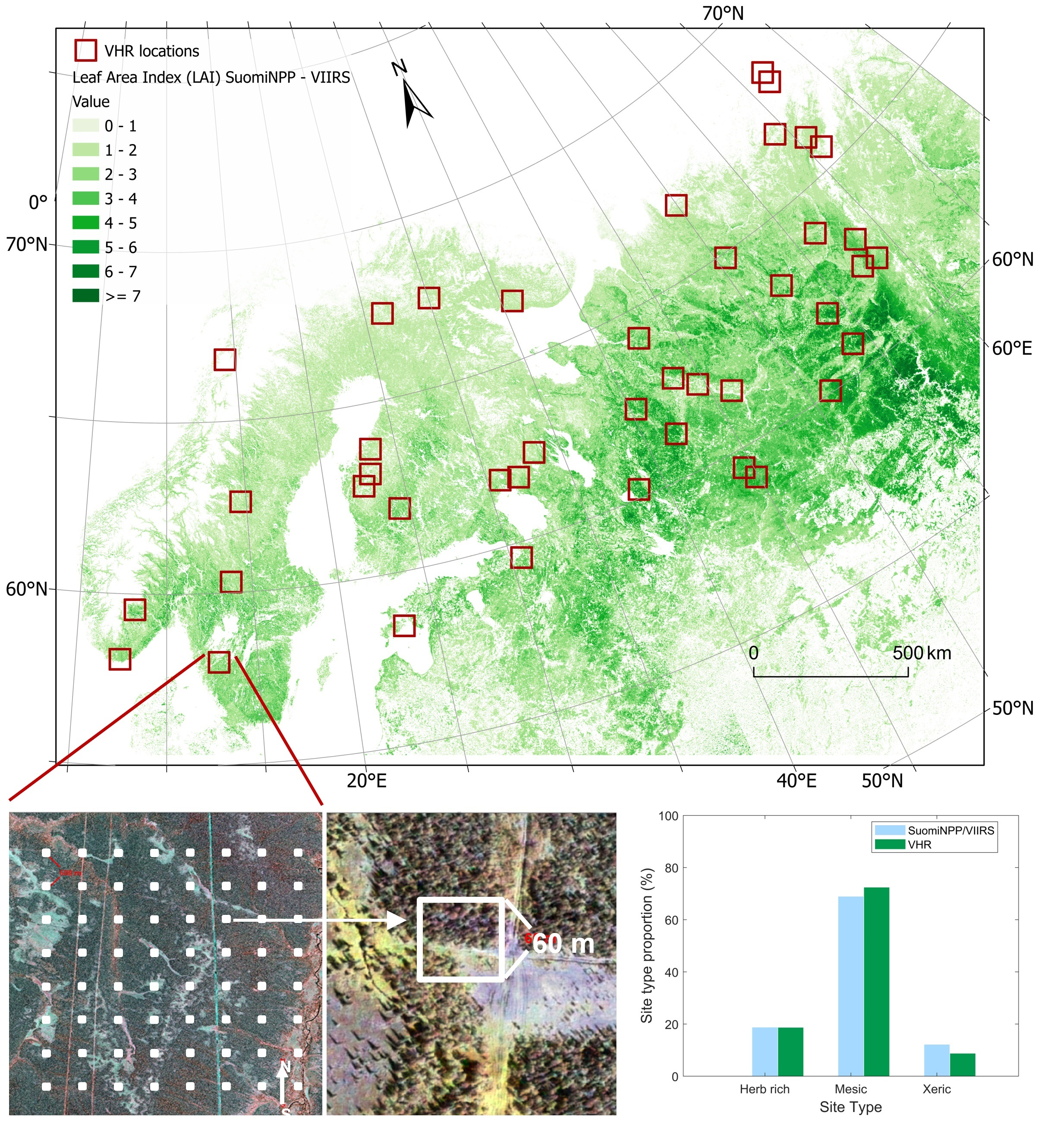
2.1. Study Area and Reference Data

The study area was the European boreal and hemi-boreal forest reaching to the coast of Norway in the west and to the Ural Mountains in the east (Figure 1). The forest covers a land area of 2,940,370 km² or 294,037,000 ha, including inland waters. The dominating species in the area are Norway spruce (Picea abies Karst.) and Scots pine (Pinus sylvestris L.). Birches (Betula sp.) are also common and abundant in western Russia. Other broadleaved species include European Aspen (Populus tremula L.), Alder (Alnus sp.), and Mountain ash (Sorbus aucuparia L.). A typical growing stock volume of mature forest in the southern part of the study site is 300–400 m³/ha. In the northern part, which reaches to the arctic tree line, the growing stock volume declines to a very low value. In Fennoscandia, most of the forest is intensively managed, while in Russia, the management intensity varies depending on the geographic region. Forest fires are common in Russia but rare in Fennoscandia [33].

The main reference data for the computation of the models for the estimation of the target variables using moderate-resolution imagery were thematic raster image maps representing the year 2013, which were available from the Natural Resources Institute Finland (Luke) [35] (Figure 2). The maps provided values for every target variable except the LAI. The maps had been computed with the k-NN method using Landsat, Spot, and other optical data with similar spatial resolutions and national forest inventory field plot data for reference [36,37]. In addition, a Finnish high-resolution version of the CORINE 2012 map on land cover classification and visual interpretations of Google Earth was used to support the labeling for the land cover classes. The CORINE high-resolution map was available at a pixel size of 25 m without generalization to the 25-hectare minimum mapping unit that is required for the official CORINE [38].

2.2. Suomi NPP VIIRS Data

Moderate-resolution data of the Image or I spectral bands of the VIIRS data were used for computing the wall-to-wall maps (

Table 1. Wavelength range of VIIRS Image (I) spectral bands.

Band I	Center Wavelength (µm)	Wavelength Range (µm)
1	0.64	0.6–0.68
2	0.865	0.85–0.88
3	1.61	1.58–1.64

). These bands have a spatial resolution of 375 m at nadir. In total, 238 Sensor Data Record (SDR data) images taken between 31 May and 30 September 2016 were downloaded from the Sodankylä receiving station of the Finnish Meteorological Institute.

The Suomi-NPP data were available as a one-day running archive in hierarchical data format (HDF5) version 5. An in-house processing line was developed for image pre-processing. The processing line consisted of software for reading the input HDF5 files and the rectification and atmospheric correction of each file. The Simplified Method for Atmospheric Correction (SMAC) program was applied to all images [39] with a constant value of 0.02 for the aerosol optical density (AOD). The straightforward application of the same constant was considered proper for the selected mosaicking method.

The images were rectified to the ETRS LAEA projection at a pixel spacing of 500 m, using a Gaussian-weighted average with a standard deviation of 250 m. The dataset was then divided into quarters according to the acquisition time to reduce the risk of possible seasonal effects on the spectral values (

Table 2. VIIRS acquisitions.

Time Range	Number of Images
13 May–19 June	58
20 June 20–11 July	53
21 August–11 September	65
12 September–30 September	62

).

Images from late July and early August were missing due to a hardware failure in the receiving station. Image mosaic composites for the four time periods were produced using the maximum normalized difference vegetation index ((NDVI), [I2 − I1]/[I2 + I1]) as the criterion. A pixel value was selected for the bands from the image that represented the maximum NDVI value. A visual analysis showed that the latter half of the growing season was affected by various artefacts for which the autumn aspect in the northern study area may have been the major reason. Pixel averages of quarters 1 and 2 were computed for the composite for map production.

2.3. VHR Data

2.3.1. Two-Stage Sampling

The sample-based data were collected using visual interpretation because no such data were available at a high resolution from the study area. Two-stage, design-based sampling using VHR imagery was chosen as the method for the provision of an alternative estimation to the mapping using VIIRS data [40,41,42]. The images were analyzed visually by an expert who was not involved in the computation of the VIIRS-based maps, and the results were not used to support the VIIRS-based mapping.

Area frame sampling was conducted within the study area to select the locations of the VHR samples. A grid of 10 km × 10 km was defined to cover the study area as the area frame for the first stage sample. A simple random sample of coordinates in the ETRS LAEA system, aimed at a selection of 40 VHR images, was conducted within the frame for the first stage sample. This sample size was considered adequate in the preliminary calculations to provide satisfactory confidence intervals for the estimated variables.

We attempted to acquire VHR images from all locations in the 10 km × 10 km grid units that included a sample point. The image database from for the years 2013–2014 from the Data WareHouse (DWH) of the European Union was checked for the availability of archived VHR images. New image acquisitions were ordered when no archived data were available. Images were accepted between 1.6. and 30.9., i.e., within the growing season. New acquisitions for the year 2015 were requested if no archive images were available (

Table 3. VHR data. New acquisitions shown in italics. Image pan-chromatic resolution was 0.5 m and multispectral resolution 2 m. Image# refers to locations shown in Figure 1. WV1 is WorldView-1; P1A is Pleiadés1A; P1B is Pleiadés1B.

Image#	Instrument	Date	Image#	Instrument	Date	Image#	Instrument	Date
1	WV1	7 August 2013	15	P1B	18 August 2015	29	P1B	21 August 2015
2	P1B	13 August 2015	16	WV1	2 June 2013	30	P1B	31 July 2015
3	P1A	19 September 2014	17	P1A	25 July 2014	31	P1A	31 July 2015
4	WV1	30 July 2013	18	WV1	28 May 2013	32	P1B	30 June 2015
5	P1B	20 September 2014	19	P1B	20 August 2015	33	WV1	25 September 2014
6	P1B	4 July 2015	20	WV1	31 May 2013	34	P1B	30 June 2015
7	P1A	16 August 2015	21	WV1	18 September 2014	35	P1A	30 June 2015
8	P1A	1 July 2015	22	P1A	6 August 2015	36	P1A	30 June 2015
9	P1A	16 August 2015	23	P1A	20 August 2015	37	P1A	7 August 2015
10	P1A	18 August 2015	24	P1B	29 July 2015	38	P1B	30 June 2015
11	P1A	3 July 2015	25	P1B	21 August 2015	39	P1A	12 August 2015
12	P1A	14 July 2014	26	P1B	24 July 2015	40	P1A	7 August 2015
13	P1B	17 August 2015	27	WV1	8 June 2014	41	WV1	8 August 2014
14	P1B	24 July 2014	28	P1B	21 August 2015	42	P1A	7 August 2015

). A possible change in forest area or structure variables between the acquisition of the VHR and VIIRS data was considered insignificant, considering the proportion of the changed area in the total area of the images. The image size for the archived images was 5 km × 5 km; however, for the new acquisitions, the minimum available size was always larger than 25 km².

The sample was supplemented with two additional subjectively chosen images from Finland. These images were available from the intensive study sites of the project and represented typical boreal and north boreal forests. Thus, the total number of VHR data was 42.

All the 42 VHR images were reprojected to the project projection used (ETRS LAEA), and their pixels were spatially aligned with the VIIRS data. Pan-sharpened natural-color and color-infrared composites were computed from the VHR images for the visual interpretation.

In the second stage, a square area of 60 m × 60 m was selected as the population unit or sample plot for the visual image interpretation. These plots formed a grid within each VHR image with a mutual distance of 600 m × 600 m (Figure 3).

In earlier tests, a distance of 800 m between plot centers was considered adequate so as to not have any major spatial autocorrelations between the plots [41]. A simulation study of a spatial autocorrelation based on a semi-variogram [43] was performed with earlier satellite-image-based maps from south and north boreal sites (Hyytiälä and Sodankylä) in Finland. The autocorrelation was not significant with the 600 m plot distance.

The location of the second-stage grid of plots was random over a finite collection of grids, meaning that a single grid was selected randomly among the grids that covered the whole image. A 5 km × 5 km archive image could include 8 × 8 = 64 s-stage sample plots. A 5 km × 5 km area from the center of a larger image from the new acquisitions was defined for the sampling. Thus, all 42 images of the random sample included 64 s-stage units. In a few cases, clouds prevented the selection of plots from a square within a VHR image. This issue was resolved by extending the sample outside the 5 km × 5 km square in the larger images from the new acquisition. The total number of the visually assessed plots was 2690. The second-stage plot size of 3600 m² made it possible to collect reference information visually from a relatively large area while minimizing subjectivity and keeping the interpretation process fast enough [41].

2.3.2. Visual Interpretation

Proportions of forest cover and land cover classes within the 60 m × 60 m plots that corresponded to the population units were defined and stored (Figure 4). The “Forest” class in Figure 4 represented a forest area in the computations. It comprised “Tree-Covered Forest” and “Open Forest”.

Open Forest meant temporarily unstocked forest, such as forest regeneration areas and burned forest areas. It was considered to meet the definition of forest as the canopy developed. Open Forest, including burned forest areas, was considered to stand out with a reasonable confidence from land cover classes that represented actual non-forest areas. However, there can be no absolute certainty that open forest can develop into an area covered by trees, and after a serious fire, open land can be a permanent result [44]. The VHR plot and VIIRS image-based estimates were compared for the class “Forest”.

Within the class “Tree-Covered Forest,” the plot crown cover, Lorey’s height, average growing stock volume, site fertility, and proportions of pine, spruce, and broadleaved trees from the volume were evaluated and registered. This analysis was considered experimental because apart from crown cover, a visual interpretation of these variables from satellite data may be unreliable. Reliable reference field data for crown cover are rarely available for comparison, making a purely visual interpretation result of this variable also uncertain. Site fertility was also assessed for the “Open Forest” class. The actual forest area within a plot was taken into consideration when the plot-based estimate was computed for the whole VHR image if a plot included forest and other land cover classes.

“Open Peat Land” was part of the “Forestry Land” class but not part of “Forest.” It was considered a non-forest area in the computations.

A custom pre-processing and analysis workflow was developed to aid in the analysis of a large quantity of visual sample plots. The pre-processing consisted of extracting image pyramids of fixed dimensions at different resolutions for each of the 2690 VHR sample plots. The plots were analyzed from natural-color and color-infrared VHR images. The color-infrared images particularly supported the assessment of the proportion of broad-leaved trees. The lengths of tree shadows aided in the estimation of the forest height. A 5 × 5 toggle grid was displayed on the plots to support the assessment of the variables within them. Each grid unit corresponded to 4% of the plot area. The plots were assessed by a professional forester who was familiar with the boreal forest but did not take part in the satellite image analysis. Training for the visual analysis was organized for the image interpreter. No reference data were available from sample plot locations. It was important to collect the VHR image sample using probability sampling, which prevented the use of of potential existing field references.

The output from the plot interpretation was a tabular file containing information on the VHR image of the plot, plot coordinates, and the results of the plot assessments.

2.4. Models for Variable Estimation

2.4.1. Land Cover Classification

The study area was divided into three south, middle, and north zones which roughly followed the hemi-boreal/south boreal, mid-boreal, and north boreal/forest tundra vegetation zones. Separate models were computed for these zones (Figure 1) [45,46].

A systematic sample of every second pixel of the VIIRS mosaic was selected, and a k-means clustering attempt for 50 classes was performed on the selected sample. The spectral mean vector and covariance matrix were computed for each cluster using its observations. The whole mosaic was then classified into spectral classes by applying the computed statistics and the maximum likelihood (ML) rule, using the Mahalanobis distance as the measure. The ML classification was the initial input for the algorithm that predicted the variables as continuous values.

The classes were labeled as land cover categories with the help of multiple information references, including the maps from Luke and the high-resolution version of the CORINE 2012 map from Finland. The labeling was supported by a visual analysis of Google Earth that covered the whole study area. The visual analysis results of the VHR data that were acquired for this study were not used to define class contents.

The number of spectral classes was eventually 49 because in the in-house implementation of k-means clustering, a cluster was rejected if the number of observations in a cluster was less than a defined threshold to which the value of 50 observations was applied. The clustering-based land cover classification was a preliminary phase for the forest cover map, which was computed in the same way as the structural variable estimates. The semi-supervised algorithm is provided in the following subsection.

2.4.2. Structural Variables

The models for the continuous-value structural variables were computed using the in-house Probability software (Figure 5) [10,41]. The reference data values from the Luke map with pixel sizes of 25 m × 25 m were sampled (Figure 2), and their averages were computed for the areas of the 500 m × 500 m VIIRS pixels. Each spectral class of the ML classification was assigned to a target value for each structural variable. These values were computed as the medians of the reference data for the growing stock volume, forest height, and site fertility class and as the averages for the proportions of pine, spruce, and broadleaved trees to ensure species proportions summing up to 100%.

The rationale of each model was assessed by plotting the structural variable values of the spectral classes in a coordinate system whose axes were the red-light and near-infrared reflectances from the VIIRS (Figure 6). In a few cases, the values were manually edited when the reflectance values and the automatically allocated reference data values of spectrally similar classes were not consistent. The possibility of manually checking and optionally editing the model was considered an advantage of the applied method compared to the commonly used machine learning methods, such as random forest [47,48].

Predictions for the structural variables were computed for every pixel of the of the VIIRS image mosaic as weighted averages of the spectral classes’ target variable values. The weight was the membership probability for a spectral class (Equation (1)). All structural variables were estimated using the same process.

$$f(x)={\displaystyle \sum _{c=1}^{N}P(c|x)f_c},$$

(1)

where $f(x)$ is the target variable value for a spectral vector $x$, $P(c|x)$ is the probability for a spectral vector $x$ to belonging to spectral class $c$, $f_c$ is the target variable value for the spectral class $c$ and $N$ the number of spectral classes. The five closest spectral classes to a spectral vector were considered in the computations.

The effective leaf area index ($LAIe$) was computed using the model shown in Equation (2) [49].

$$LAIe=0.27+0.25\times RSR,$$

(2)

where $RSR=\frac{I2}{I1}\times \frac{I{3}_{max}-I3}{I{3}_{max}-I{3}_{min}}, \mathrm{and}$ $I1, I2$, and $I3$ are the atmospherically corrected reflectances of the VIIRS red, near-infrared, and short-wave infrared bands. $I{3}_{max}$ represents the reflectance of $I3$ on open and $I{3}_{min}$ on closed canopies. These values were selected manually from the VIIRS mosaic.

The forest cover map was also computed using the Probability method by applying a forest cover of 0% or 100% to the ML classes. The final forest map was obtained from the continuous-value prediction by applying a threshold of 50 % to the predicted percentage of forest cover.

An evaluation of the initial results using the three vegetation zone strata showed that the model for the southern zone was unfeasible partly due to the scarcity of reference data. The predictions that were computed using the middle and northern zones provided seamless estimates at the zone borders in Finland. However, a clearly visible border appeared in the eastern parts of the boreal region. As the values predicted with the middle zone model also produced consistent values for the northernmost areas, the model for the north zone was eventually abandoned, and the model for the middle zone was applied to the whole VIIRS mosaic.

Water was extracted from the predictions using the water layer of a map by the University of Maryland [5].

2.5. Computation of Means and Their Confidence Intervals

2.5.1. Means and Confidence Intervals for Target Variables for VHR Image Areas

For each VHR image, the estimates of the expected values and their 95% confidence intervals for the forest area, site fertility, and continuous variables were computed from the results of assessing the 60 m × 60 m plots by applying simple random sampling formulas. Forest proportions within the plots were considered when the results were computed for the VHR images.

The estimates of the VIIRS map were sampled for the VHR image areas from the bounding shape (usually a square) that covered the 64 VHR image plots of 60 m × 60 m. This enabled a comparison of the VHR- and VIIRS-based results for the areas of the 42 VHR images.

No data were available from the VHR image assessment to compare with the VIIRS-based LAI. Instead, the correlation of the LAI values from the VIIRS was compared with the estimated crown cover percentage from the visual VHR image interpretation.

2.5.2. Means and Confidence Intervals for Target Variables for Whole Study Area from VHR Images

The forest area percentage and its 95% confidence interval for the whole study area were computed by summing up the forest areas of the individual VHR images using formulas for a two-stage sampling design [40], equations below:

The sampling fraction in the 1st stage: $f_1=\frac{n}{N}$

The sampling fraction in the 2nd stage: $f_2=\frac{m}{M}$, (Note: $f_2=\frac{m}{M}\le \frac{1}{100}$)

The value of forest area in the $i$th VHR image and in the $j$th plot of that image: $y_{ij}$, $i=1,\dots ,n$, $j=1,\dots ,m$ where

• $N$ is the size of the sampling frame of all possible VHR images. $f_1=\frac{n}{N}\approx 0$ because $N$ is a very large number due to the large study area.
• $M$ is the number of possible plot locations within each VHR image: ($M\ge 6400$).
• $n=42$ is the number of VHR images;
• $m=64$ is the number of selected plots within a VHR image.

The average forest area of a variable of the ith VHR image in the 2nd stage: ${\overline{y}}_i=\frac{1}{m}{{\displaystyle \sum }}_{j=1}^m{y}_{ij}$

The average for the whole area: $\stackrel{=}{y}=\frac{1}{nm}{{\displaystyle \sum }}_{i=1}^n{{\displaystyle \sum }}_{j=1}^m{y}_{ij}=\frac{1}{n}{{\displaystyle \sum }}_{i=1}^n\left(\frac{1}{m}{{\displaystyle \sum }}_{j=1}^m{y}_{ij}\right)=\frac{1}{n}{\displaystyle \sum }_{i=1}^n{\overline{y}}_i$.

The variance of the average: $v\left(\stackrel{=}{y}\right)=\frac{1-f_1}{n}{s}_1^2+\frac{f_1\left(1-f_2\right)}{nm}{s}_2^2$, (note: $f_1\approx 0\Rightarrow v\left(\stackrel{=}{y}\right)=\frac{1}{n}{s}_1^2$) where $s_1^2=\frac{1}{n-1}{{\displaystyle \sum }}_{i=1}^n{\left({\overline{y}}_i-\stackrel{=}{y}\right)}^2$ and $s_2^2=\frac{1}{n}{{\displaystyle \sum }}_{i=1}^n\left(\frac{1}{m-1}{{\displaystyle \sum }}_{j=1}^m{\left(y_{ij}-{\overline{y}}_i\right)}^2\right)$.

The predictions for forest area and structural variables of the VIIRS map were compared with the estimates from the VHR image interpretation for the whole study area. The predictions were also compared at the national level with the Finnish and Swedish statistical data from the national forest inventories. An additional comparison was made by extracting the areas of the VHR images from the VIIRS maps. This comparison provided information on the local uncertainty and the extent of averaging in the VIIRS-based prediction.

3. Results with Accuracy Considerations

3.1. Forest Variables for the Whole Study Area, Finland, and Sweden

The forest area prediction from the VIIRS map (Figure 7) was close to the average of the estimates from the VHR plots (

Table 4. Forest area and structural variables in VIIRS map and from VHR plots.

Variable	VIIRS Map	VHR 95% Ci-Low	Expected Value	VHR 95% Ci-High
Forest area (km2)	2,140,589	1,840,672	2,114,126	2,416,984
Forest proportion (%) *	72.8	62.6	71.9	82.2
Growing stock volume (1000m3) *	23,332,420	152,960	217,332	296,081
Growing stock volume (m3/ha) *	109.0	83.1	102.8	122.5
Forest height (m)	12.5	10.2	11.9	13.6
Conifer proportion (%)	74.9	63.7	68.5	73.4
BL proportion (%)	25.1	26.6	31.5	36.3

* including Forest, Peat forest (in VHR data), and Open Forest.

). It was 1.2% or 26,463 km² higher than the expected forest area estimated from the VHR plots. In the VIIRS classification, an attempt was made to separate the class Open Forest, i.e., the recent clear cuts or burned forest areas in Russia, for instance. Part of the open bogs were also included in the Open Forest class due to the relatively coarse resolution of the VIIRS instrument. The proportion of Open Forest was 5.4% from the VHR data, which did not include open bogs (

Table 5. Distribution of forest area to sub-classes from VHR plot data and their growing stock volume values.

Class	Forest Proportion from VHR Plots, (%)	Area, 95% Confidence Interval (%)	$\mathbf{V},\mathbf{Expected}\mathbf{Value}({\mathbf{m}}^3/\mathbf{ha})$	V, 95% Confidence Interval
Mineral Soil Forest	58.3	(48.8, 67.7)	125.3	(101.6, 149.0)
Peat Forest	8.2	(4.6, 11.8)	11.0	(7.1, 14.9)
Mineral Soil + Peat Forest	66.5	(57.7, 75.2)	111.2	(89.9, 132.4)
Open Forest	5.4	(3.3, 7.5)	0.0	n/a
Mineral Soil + Peat Forest and Open Forest	71.9	(62.6, 82.2)	102.8	(83.1, 122.5)

).

Similar to forest area, the VIIRS-based forest volume and height also fit into the 95% confidence interval of the VHR estimation (Figure 8 and Figure 9). The conifer proportion from VIIRS was higher, and the broadleaved tree proportion was lower than in the VHR image assessment. They did not fit into the 95% confidence limits.

The VIIRS map was also compared to the national forest inventory statistical data from Finland (

Table 6. VIIRS map totals (mean) and Finnish national forest inventory statistics for the whole country.

Variable	VIIRS Map	NFI FI
Forest area (km2)	258,346	226,600 1
Forest proportion (%) 2	77.0	67.0
Growing stock volume (1000 m3)	2,707,466	2,506,000 1
Growing stock volume (m3/ha)	104.8	110.6 1
Conifer proportion (%)	77.5	80.0 3
BL proportion (%)	22.6	20.0 3

¹ Including Forest Land—capability 1 m³/ha/year or more, Poorly Productive Forest Land—capability 0.1–1 m³/ha/year. ² Computed from area of the country including inland waters. ³ Proportions of growing stock volume. Source for NFI FI data: [50].

) and Sweden (

Table 7. Suomi NPP map totals (mean) and Swedish national forest inventory statistics for the whole country.

Variable	VIIRS Map	NFI SE
Forest area (km2)	320,879	301,910 1
Forest proportion (%) 2	71.6	67.0
Growing stock volume (1000 m3)	3,451,799	3,574,000
Growing stock volume (m3/ha)	107.5	118.4 1
Conifer proportion (%)	77.8 3	80.4 3
BL proportion (%)	22.2 3	19.6 3

¹ Including Forest land and Other wooded land. ² Computed from area of the country including inland waters. ³ Proportions of growing stock volume. Source for NFI SE: [51].

).

In Finland, the forest area on the VIIRS map was 31,746 km² or 14.0% higher, corresponding to the 10% difference in the proportion of forest, than the areas of the Forest Land and Poorly Productive Forest Land classes from the national forest inventory data. The VIIRS prediction was close to the area of Forestry Land, with an underestimation of 1.3%. The Forestry Land also included an area of Unproductive Land measuring 32,940 km² or 9.7% of the area of the country. It comprises mostly open bogs and, among other things, the top areas of the arctic hills in the northern part of the country.

The total growing stock volume was overestimated by 8.0% on the VIIRS maps (Figure 8). The conifer/broadleaved tree proportions were close to the NFI results when the variables compared were the proportions of tree species in the volume (Table 6). We considered the proportion of the volume more applicable for the comparison than species dominance because the dominance concerns the main species only, ignoring mixtures of secondary species. The conifer dominance was 89.5% in the Finnish NFI data if the area was used as the criterion instead of the volume.

The VIIRS map matched with the Swedish forest statistics better than with the Finnish statistics. The forested area was overestimated by 6.3% and the growing stock volume was underestimated by 3.4%, respectively. As in Finland, the match with the conifer/broadleaved tree proportions was good when the proportions from the NFI data illustrated the proportions of the growing stock volume.

3.2. Comparison of VIIRS Map and VHR Plot Assessment by VHR Image Areas

Figure 10 shows the comparison between the variables estimated from the VHR plots and the VIIRS-based predictions with each VHR image. The VHR-based estimates converged well with VIIRS results except that they were lower on average. For the forest area, images #10, 12, 15, 32, and 36 showed much lower values from the VHR plots than from the VIIRS map. Image #12 was from a fragmented landscape in Estonia, whereas all other images were from the northern latitudes, and images #15, 32, and 36 were from close to the forest line. The VHR image interpreter had considered a large proportion of the plots on the images to represent shrubland, whereas the same area was largely classified as forest on the VIIRS map. Image #10 represented a barren northern boreal pine forest with abundant lichen undergrowth.

Despite the tendency toward an overestimation of the VIIRS map, the binary forest cover estimations, which were below or above 50% for the areas of VHR images, matched well because the forest recognition between the VHR assessment and the VIIRS map was 88.1%. This was at the same level as the best results in the global forest cover surveys using Earth observation [15].

The VIIRS-based growing stock volume predictions varied much less than the VHR estimates. In 13/42 cases only, the VIIRS prediction fit within the 95% confidence interval from the VHR analysis. However, the correlation r = 0.7 between the VIIRS and VHR estimates was reasonably high, and the averages were close to each other.

A comparison of the VIIRS and VHR-based height estimates showed a very similar pattern to the volume predictions. The VHR confidence interval match with the VIIRS map was 14/42. The averages were practically the same.

The conifer proportion estimates were higher from the VIIRS, and the broadleaved tree proportion estimates were lower than from the VHR data, although the average difference was relatively small. The confidence interval agreements were 17/42 and 15/42, respectively. The averaging nature of the VIIRS estimation was also apparent in the species estimation. The agreement for the dominant species was good, 88.1% for the conifer dominance and 90.5% for the broadleaved trees, respectively, using 50% as the criterion for species dominance. The agreement was 61.9% if the mixed forest class was included in addition to the pure conifer or broadleaved forests. A threshold of 75% was applied for the pure forests when the mixed forest class was included.

The predictions of site fertility class distributions using VIIRS were in line with the estimates using VHR data when the fertility was grouped into three main classes: herb rich, mesic, and xeric (Figure 11). The match was also good for many individual VHR image areas (Figure 12).

The scatterplots between the VHR- and VIIRS-based estimates demonstrate a clear correlation between them but also the strong averaging in the VIIRS results. The crown cover assessment from the VHR imagery was compared with the VIIRS-based LAI because no attempt was made to evaluate the LAI from the VHR data (Figure 13 and Figure 14).

4. Discussion

4.1. General Approach

The two independent estimation procedures, the Probability method using Suomi NPP VIIRS imagery and the visual interpretation of sample plots from VHR imagery, led to similar results for the forest variables for the whole study area. The reference data for the computed VIIRS map were available from raster maps that had been computed via the interpolation of the NFI field sample plot data from Finland using the k-NN method. The satellite imagery for these reference maps was obtained from Landsat and other satellites, providing a similar spatial resolution.

The VHR data were collected using a two-stage random sampling design which can be considered practically unbiased. The visual interpretation of the plots could have included a systematic error of an unknown magnitude. However, we considered the estimation of forest cover from the VHR data to be reliable due to their high spatial resolution. Similar studies using the visual interpretation of satellite imagery have used lower-resolution data from Landsat or Sentinel as the primary image source [15,16]. Unlike several other earlier projects, we applied non-stratified random sampling for the VHR data [52,53]. The earlier studies focused on one or a few variables, but in our study, for the estimation of five variables, a simple random sampling was considered more robust. In addition, the whole study area had a high forest cover proportion and there was no obvious foundation for defining the strata.

4.2. VIIRS Map and VHR Sample Agreement for Whole Area

The VIIRS predictions for forest proportion and height were very close to the expected values from the VHR estimation, and the average growing stock volumes were also similar. The proportion of conifers from the VIIRS map was higher than from the VHR plots, and the proportion of broadleaved trees was correspondingly lower, being outside the VHR-data-based 95% confidence limits. The confidence interval was narrowest for the conifers at 14.2% from the expected value and broadest for the volume at 38.3%.

The broadleaved tree proportion estimate increased from 22.0% for the Nordic countries to 32.1% for Russia when computed as the average of VHR images from those areas. In the VIIRS-based estimation, the change was from 20.6% to 24.1%, respectively (Figure 1 and Figure 9). The VIIRS-based predictions could be too low in Russia because they were computed using Finnish reference data that reflected the forest management regime in the Nordic countries. The same increasing trend could be observed for volume. However, these observations should be considered with caution because the VHR sample size for the Nordic countries was only twelve, and in Finland, for instance, four of the five images were sampled from regions with lower growing stock volumes.

4.3. Agreement with NFI Data and Worldcover

The VIIRS map overestimated the forest area proportion by 10.0% points in Finland and 4.6% points in Sweden when compared to the NFI data. These differences are clearly beyond the NFI’s results because their 95% intervals are below ±1% of the expected value in Finland and ±2% of the expected value in Sweden, respectively [37,51]. The average growing stock volumes were underestimated, which reduced the overestimation of the total growing stock volume compared to the error for the forest area in Finland. A major part of the Finnish landscape is very fragmented, with plenty of small lakes, agricultural land with small field sizes, and open bogs in the northern part of the country. This may be a reason for the overestimation of forest area using the VIIRS data with a pixel size of 500 m. In Sweden, the compensation led to an underestimate of the total volume.

The forest area predictions were also compared with the recent Worldcover map [4]. It showed a clearly lower forest proportion of 64.9% than the VIIRS map. It was also lower than the expected value from the VHR estimation but fit within its 95% confidence limits. The Worldcover estimate for forest area was 3.0% points lower compared to the Finnish NFI data and 3.4% points lower for Sweden. The class for forest in Worldcover is called Tree Cover; this suggests that it does not consider the temporarily unstocked forest. This led to the underestimation compared to the VHR data-based result and national forest inventories.

A comparison of the uncertainty of the VIIRS maps and the maps with space-borne GLAS lidar data as key information sources should be performed with caution without comparing the actual maps. However, the large differences between the GLAS-based mappings in [23,24] already show that their approaches are not error-free. In our study, the VIIRS maps and VHR assessment showed similar results.

4.4. Agreement at VHR Image Locations

When selected at the locations of the VHR images only, the average of the VIIRS-based predictions for the structural variables and tree species was very similar to the average including all the VIIRS pixels. An exception was forest area, for which the VIIRS prediction average was 10.7% points higher than the VHR estimate, although the estimates were close to each other when all the VIIRS pixels of the study area were considered.

As expected, the VIIRS-based maps strongly averaged the predictions because a VIIRS pixel corresponded to an area of 25 ha, while individual trees were visible in the VHR data. The uncertainty of the VIIRS estimation at the VHR image locations, corresponding to 10 × 10 VIIRS pixels, can be considered high. The VIIRS maps could show the relative differences in the structural variables, as demonstrated in the correlation coefficients and scatterplots with the VHR results, with r = 0.85 for the forest area and from r = 0.69 to r = 0.74 for the other variables, including the crown cover vs. LAI. Despite the significantly reduced dynamic range in the VIIRS maps compared with the VHR image assessment, the averages of the structural variables were close, suggesting a relatively unbiased estimation at a more local level as well. Using the 10-meter resolution of the Sentinel-2 satellite reduces the averaging, but saturation can still be observed with increasing volume values above 200 m³/ha [28].

Space-borne lidar data obtained using the GEDI instrument provides a higher dynamical range for height than image data with a larger pixel size and could consequently lead to better local estimation for growing stock volume and biomass as well; however, the GEDI-based models have had RMSEs as high as nine meters [26]. Operational space-borne lidar instruments that would be applicable for forestry are not foreseen in the near future.

The good agreement of the VIIRS and VHR estimates for the main tree species groups, 88.1% for conifers and 90.5% for broadleaved trees at the VHR image areas, suggest that the mapping of the dominant group is reliable from data of a coarser resolution. The reliability for the mixed forest class was lower, which has also been reported in earlier studies [16].

The classification of site fertility into three classes matched well for the whole study area in the VIIRS and VHR results because their class-wise differences were only a few percentage points. The classifications also often matched well at the level of single VHR images. This is an important result because the site fertility class affects forest growth and can be a key variable in the process models for primary production [54]. Satellite image-based estimation can be used as input for those models [55].

4.5. Calibration Tests

The interpretation of the forest area from the VHR images can be considered reliable. Therefore, two approaches to calibrate the VIIRS estimation were experimentally tested. One approach was to increase the threshold for the forest area from 50.0% to 60.7%, corresponding to the average differences between the VIIRS and VHR estimates at the areas of the VHR images. The other approach was to compute a linear regression model between the forest areas of the individual VHR images as the predicted variable and the VIIRS map forest areas from the same locations as the predictors. Both approaches led to an approximately one-percent reduction in the forest area estimates for Finland and Sweden. The reduction was considered so low that the results are not presented in this paper in detail. The calibration was also against the leading principle of this study on the comparison of independent estimations.

5. Conclusions

Based on the results of this study, we can confirm our hypothesis that using two independent approaches, i.e., VIIRS-image-based wall-to-wall mapping and two-stage sampling and visual interpretation from VHR imagery, improves the credibility of remote-sensing-based surveys. The two estimations probably gave realistic results of the central forest variables for the European boreal forest from national to continental levels because they led to similar results. This conclusion can be made despite the fact that no field reference data were available for most of the area. For the forest area, the VIIRS map and VHR sample estimates were very close. Additionally, for the height and growing stock volume, the VIIRS estimates fit within the confidence intervals computed from the VHR sample. The reference data from Finland may have underestimated the broadleaved tree proportion in Russia. The relatively good agreement between the VIIRS maps and the national forest inventory statistical data in Finland and Sweden support the conclusion of the low bias in our estimation.

According to our results, optical data of a coarser resolution, e.g., 100–500 m, are applicable for the estimation and mapping of a forest area and central structural variables at the regional to national levels. A model computed using reference data from a small part of the area of interest can provide satisfactory predictions for a much larger area with a similar biome. Our concept could be directly applied also to higher-resolution wall-to-wall satellite data, such as Sentinel-2 imagery. Part of the VHR image plots could also be measured on the ground, which would further improve the reliability and reduce bias in wall-to-wall mapping through calibration. A similar concept has been implemented using visual analysis of aerial photos and two-phase sampling [56].

An independent parallel estimation using a sample of VHR imagery can provide more certainty to the wall-to-wall mapping using lower-resolution data when the collection of field data is not a feasible alternative. The VHR data also make it possible to consider the temporarily unstocked forest that is often ignored in satellite-image-based mapping, leading to the underestimation of forest area.

References

1. FAO. Global Forest Resources Assessment 2020 Key Findings; FAO: Rome, Italy, 2020. [Google Scholar]
2. Nabuurs, G.J.; Masera, K.O.; Andrasko, P.; Benitez-Ponce, R.; Boer, M.; Dutschke, E.; Elsiddig, J.; Ford-Robertson, P.; Frumhoff, T.; Karjalainen, O.; et al. Chapter 9: Forestry—AR4 WGIII. Available online: https://archive.ipcc.ch/publications_and_data/ar4/wg3/en/ch9.html (accessed on 28 December 2022).
3. Lier, M.; Köhl, M.; Korhonen, K.T.; Linser, S.; Prins, K.; Talarczyk, A. The New EU Forest Strategy for 2030: A New Understanding of Sustainable Forest Management? Forests 2022, 13, 245. [Google Scholar] [CrossRef]
4. Zanaga, D.; Van De Kerchove, R.; De Keersmaecker, W.; Souverijns, N.; Brockmann, C.; Quast, R.; Wevers, J.; Grosu, A.; Paccini, A.; Vergnaud, S.; et al. ESA WorldCover 10 m 2020 V100. 2021. Available online: https://zenodo.org/record/5571936 (accessed on 17 January 2023).
5. Hansen, M.C.; Potapov, P.V.; Moore, R.; Hancher, M.; Turubanova, S.A.; Tyukavina, A.; Thau, D.; Stehman, S.V.; Goetz, S.J.; Loveland, T.R.; et al. High-Resolution Global Maps of 21st-Century Forest Cover Change. Science 2013, 342, 850–853. [Google Scholar] [CrossRef] [PubMed] [Green Version]
6. Kangas, A.; Gove, J.H.; Scott, C.T. Introduction; Springer: Dordrecht, The Netherlands, 2006; pp. 3–11. [Google Scholar]
7. McRoberts, R. The National Forest Inventory of the United States of America. J. For. Sci. 2008, 24, 127–135. [Google Scholar]
8. Tomppo, E.; Olsson, H.; Ståhl, G.; Nilsson, M.; Hagner, O.; Katila, M. Combining National Forest Inventory Field Plots and Remote Sensing Data for Forest Databases. Remote Sens. Environ. 2008, 112, 1982–1999. [Google Scholar] [CrossRef]
9. Liu, H.; Gong, P.; Wang, J.; Wang, X.; Ning, G.; Xu, B. Production of Global Daily Seamless Data Cubes and Quantification of Global Land Cover Change from 1985 to 2020—IMap World 1.0. Remote Sens. Environ. 2021, 258, 112364. [Google Scholar] [CrossRef]
10. Häme, T.; Stenberg, P.; Andersson, K.; Rauste, Y.; Kennedy, P.; Folving, S.; Sarkeala, J. AVHRR-Based Forest Proportion Map of the Pan-European Area. Remote Sens. Environ. 2001, 77, 76–91. [Google Scholar] [CrossRef]
11. Shimada, M.; Itoh, T.; Motooka, T.; Watanabe, M.; Shiraishi, T.; Thapa, R.; Lucas, R. New Global Forest/Non-Forest Maps from ALOS PALSAR Data (2007–2010). Remote Sens. Environ. 2014, 155, 13–31. [Google Scholar] [CrossRef]
12. Martone, M.; Rizzoli, P.; Wecklich, C.; González, C.; Bueso-Bello, J.L.; Valdo, P.; Schulze, D.; Zink, M.; Krieger, G.; Moreira, A. The Global Forest/Non-Forest Map from TanDEM-X Interferometric SAR Data. Remote Sens. Environ. 2018, 205, 352–373. [Google Scholar] [CrossRef]
13. Pulella, A.; Santos, R.A.; Sica, F.; Posovszky, P.; Rizzoli, P. Multi-Temporal Sentinel-1 Backscatter and Coherence for Rainforest Mapping. Remote Sens 2020, 12, 847. [Google Scholar] [CrossRef] [Green Version]
14. Ruiz-Ramos, J.; Marino, A.; Boardman, C.; Suarez, J. Continuous Forest Monitoring Using Cumulative Sums of Sentinel-1 Timeseries. Remote Sens. 2020, 12, 3061. [Google Scholar] [CrossRef]
15. Congalton, R.G.; Gu, J.; Yadav, K.; Thenkabail, P.; Ozdogan, M. Global Land Cover Mapping: A Review and Uncertainty Analysis. Remote Sens. 2014, 6, 12070–12093. [Google Scholar] [CrossRef] [Green Version]
16. Schepaschenko, D.; See, L.; Lesiv, M.; McCallum, I.; Fritz, S.; Salk, C.; Moltchanova, E.; Perger, C.; Shchepashchenko, M.; Shvidenko, A.; et al. Development of a Global Hybrid Forest Mask through the Synergy of Remote Sensing, Crowdsourcing and FAO Statistics. Remote Sens. Environ. 2015, 162, 208–220. [Google Scholar] [CrossRef]
17. Schuck, A.; Päivinen, R.; Häme, T.; Van Brusselen, J.; Kennedy, P.; Folving, S. Compilation of a European Forest Map from Portugal to the Ural Mountains Based on Earth Observation Data and Forest Statistics. For. Policy Econ. 2003, 5, 187–202. [Google Scholar] [CrossRef]
18. Sexton, J.O.; Song, X.-P.; Feng, M.; Noojipady, P.; Anand, A.; Huang, C.; Kim, D.-H.; Collins, K.M.; Channan, S.; Dimiceli, C.; et al. Global, 30-m Resolution Continuous Fields of Tree Cover: Landsat-Based Rescaling of MODIS Vegetation Continuous Fields with Lidar-Based Estimates of Error. Int. J. Digit. Earth 2013, 8947, 130321031236007. [Google Scholar] [CrossRef] [Green Version]
19. Pflugmacher, D.; Rabe, A.; Peters, M.; Hostert, P. Mapping Pan-European Land Cover Using Landsat Spectral-Temporal Metrics and the European LUCAS Survey. Remote Sens. Environ. 2019, 221, 583–595. [Google Scholar] [CrossRef]
20. Büttner, G. CORINE Land Cover and Land Cover Change Products. Remote Sens. Digit. Image Process. 2014, 18, 55–74. [Google Scholar]
21. Hame, T.; Salli, A.; Andersson, K.; Lohi, A. A New Methodology for the Estimation of Biomass of Conifer dominated Boreal Forest Using NOAA AVHRR Data. Int. J. Remote Sens. 1997, 18, 3211–3243. [Google Scholar] [CrossRef]
22. Miettinen, J.; Carlier, S.; Häme, L.; Mäkelä, A.; Minunno, F.; Penttilä, J.; Pisl, J.; Rasinmäki, J.; Rauste, Y.; Seitsonen, L.; et al. Demonstration of Large Area Forest Volume and Primary Production Estimation Approach Based on Sentinel-2 Imagery and Process Based Ecosystem Modelling. Int. J. Remote. Sens. 2021, 42, 9492–9514. [Google Scholar] [CrossRef]
23. Saatchi, S.S.; Harris, N.L.; Brown, S.; Lefsky, M.; Mitchard, E.T.A.; Salas, W.; Zutta, B.R.; Buermann, W.; Lewis, S.L.; Hagen, S.; et al. Benchmark Map of Forest Carbon Stocks in Tropical Regions across Three Continents. Proc. Natl. Acad. Sci. USA 2011, 108, 9899–9904. [Google Scholar] [CrossRef] [Green Version]
24. Baccini, A.; Goetz, S.J.; Walker, W.S.; Laporte, N.T.; Sun, M.; Sulla-Menashe, D.; Hackler, J.; Beck, P.S.A.; Dubayah, R.; Friedl, M.A.; et al. Estimated Carbon Dioxide Emissions from Tropical Deforestation Improved by Carbon-Density Maps. Nat. Clim. Chang. 2012, 2, 182–185. [Google Scholar] [CrossRef]
25. Avitabile, V.; Herold, M.; Heuvelink, G.B.M.; Lewis, S.L.; Phillips, O.L.; Asner, G.P.; Armston, J.; Ashton, P.S.; Banin, L.; Bayol, N.; et al. An Integrated Pan-Tropical Biomass Map Using Multiple Reference Datasets. Glob. Chang. Biol. 2016, 22, 1406–1420. [Google Scholar] [CrossRef] [PubMed] [Green Version]
26. Potapov, P.; Li, X.; Hernandez-Serna, A.; Tyukavina, A.; Hansen, M.C.; Kommareddy, A.; Pickens, A.; Turubanova, S.; Tang, H.; Silva, C.E.; et al. Mapping Global Forest Canopy Height through Integration of GEDI and Landsat Data. Remote Sens. Environ. 2021, 253, 112165. [Google Scholar] [CrossRef]
27. Duncanson, L.; Kellner, J.R.; Armston, J.; Dubayah, R.; Minor, D.M.; Hancock, S.; Healey, S.P.; Patterson, P.L.; Saarela, S.; Marselis, S.; et al. Aboveground Biomass Density Models for NASA’s Global Ecosystem Dynamics Investigation (GEDI) Lidar Mission. Remote Sens. Environ. 2022, 270, 112845. [Google Scholar] [CrossRef]
28. Astola, H.; Häme, T.; Sirro, L.; Molinier, M.; Kilpi, J. Comparison of Sentinel-2 and Landsat 8 Imagery for Forest Variable Prediction in Boreal Region. Remote Sens. Environ. 2019, 223, 257–273. [Google Scholar] [CrossRef]
29. Santoro, M.; Cartus, O.; Carvalhais, N.; Rozendaal, D.M.A.; Avitabile, V.; Araza, A.; de Bruin, S.; Herold, M.; Quegan, S.; Rodríguez-Veiga, P.; et al. The Global Forest Above-Ground Biomass Pool for 2010 Estimated from High-Resolution Satellite Observations. Earth Syst. Sci. Data 2021, 13, 3927–3950. [Google Scholar] [CrossRef]
30. Cajander, A.K. Forest Types and Their Significance. Silva Fenn. 1949, 56, 7396. [Google Scholar] [CrossRef] [Green Version]
31. Lambin, E.F.; Mayaux, P. Calibration of Tropical Forest Area Estimates at Coarse Spatial Resolution with Fine Resolution Data. Int. Geosci. Remote Sens. Symp. 1995, 2, 1003–1005. [Google Scholar] [CrossRef]
32. Deppe, F. Forest Area Estimation Using Sample Surveys and Landsat MSS and TM Data. Photogramm. Eng. Remote Sens. 1998, 64, 285–292. [Google Scholar]
33. Kuusela, K. The Dynamics of Boreal Coniferous Forests; SITRA: Manama, Bahrain, 1990; ISBN 951-563-274-9. [Google Scholar]
34. INSPIRE Infrastructure for Spatial Information in Europe. D2.8.I.2 Data Specification on Geographical Grid Systems-Technical Guidelines. 2014. Available online: https://inspire.ec.europa.eu/documents/Data_Specifications/INSPIRE_Specification_GGS_v3.0.1.pdf (accessed on 17 January 2023).
35. The Multi-Source National Forest Inventory of Finland—Methods and Results 2015—Jukuri. Available online: https://jukuri.luke.fi/handle/10024/543826 (accessed on 6 April 2022).
36. Katila, M.; Rajala, T.; Kangas, A. Assessing Local Trends in Indicators of Ecosystem Services with a Time Series of Forest Resource Maps. Silva Fenn. 2020, 54, 1–19. [Google Scholar] [CrossRef]
37. Korhonen, K.T.; Ahola, A.; Heikkinen, J.; Henttonen, H.M.; Hotanen, J.-P.; Ihalainen, A.; Melin, M.; Pitkänen, J.; Räty, M.; Sirviö, M.; et al. Forests of Finland 2014–2018 and Their Development 1921–2018. Silva Fenn. 2021, 55, 10662. [Google Scholar] [CrossRef]
38. Härmä, P.; Teiniranta, R.; Törmä, M.; Repo, R.; Järvenpää, E. (22) (PDF) The Production of Finnish CORINE Land Cover 2000 Classification. Available online: https://www.researchgate.net/publication/253513467_The_production_of_Finnish_CORINE_land_cover_2000_classification (accessed on 8 April 2022).
39. Rahman, H.; Dedieu, G. SMAC: A Simplified Method for the Atmospheric Correction of Satellite Measurements in the Solar Spectrum. Int. J. Remote Sens. 1994, 15, 123–143. [Google Scholar] [CrossRef]
40. Cochran, W.G. Sampling Techniques, 3rd ed.; John Wiley & Sons: Hoboken, NJ, USA, 1977; ISBN 0-471-16240-X. [Google Scholar]
41. Häme, T.; Kilpi, J.; Ahola, H.A.; Rauste, Y.; Antropov, O.; Rautiainen, M.; Sirro, L.; Bounpone, S. Improved Mapping of Tropical Forests with Optical and SAR Imagery, Part I: Forest Cover and Accuracy Assessment Using Multi-Resolution Data. IEEE J. Sel. Top. Appl. Earth Obs. Remote Sens. 2013, 6, 74–91. [Google Scholar] [CrossRef]
42. Olofsson, P.; Foody, G.M.; Herold, M.; Stehman, S.V.; Woodcock, C.E.; Wulder, M.A. Good Practices for Estimating Area and Assessing Accuracy of Land Change. Remote Sens. Environ. 2014, 148, 42–57. [Google Scholar] [CrossRef]
43. Zhang, J.; Goodchild, M.F. Uncertainty in Geographical Information; CRC Press: Boca Raton, FL, USA, 2002. [Google Scholar] [CrossRef]
44. Hansen, W.D.; Fitzsimmons, R.; Olnes, J.; Williams, A.P. An Alternate Vegetation Type Proves Resilient and Persists for Decades Following Forest Conversion in the North American Boreal Biome. J. Ecol. 2021, 109, 85–98. [Google Scholar] [CrossRef]
45. Larsen, J.A. The Boreal Ecosystem; Academic Press: Cambridge, MA, USA, 1980; ISBN 0-12-436880-8. [Google Scholar]
46. Henttonen, H.M.; Nöjd, P.; Suvanto, S.; Heikkinen, J.; Mäkinen, H. Size-Class Structure of the Forests of Finland during 1921–2013: A Recovery from Centuries of Exploitation, Guided by Forest Policies. Eur. J. For. Res. 2020, 139, 279–293. [Google Scholar] [CrossRef] [Green Version]
47. Ho, T.K. The Random Subspace Method for Constructing Decision Forests. IEEE Trans. Pattern Anal. Mach. Intell. 1998, 20, 832–844. [Google Scholar] [CrossRef] [Green Version]
48. Breiman, L. Random Forests. Mach. Learn. 2001, 45, 5–32. [Google Scholar] [CrossRef] [Green Version]
49. Heiskanen, J.; Rautiainen, M.; Korhonen, L.; Mõttus, M.; Stenberg, P. Retrieval of Boreal Forest LAI Using a Forest Reflectance Model and Empirical Regressions. Int. J. Appl. Earth Obs. Geoinf. 2011, 13, 595–606. [Google Scholar] [CrossRef]
50. Finnish Statistical Yearbook of Forestry | Natural Resources Institute Finland. Available online: https://www.luke.fi/en/statistics/about-statistics/statistical-publications/finnish-statistical-yearbook-of-forestry (accessed on 9 September 2022).
51. Nilsson, P.; Roberge, C.; Fridman, J.; Wulff, S. Skogsdata 2019; Official Statistics of Sweden: Örebro, Sweden, 2019. [Google Scholar]
52. Global Forest Resources Assessments, FAO. Available online: https://www.fao.org/forest-resources-assessment/remote-sensing/fra-2020-remote-sensing-survey/methodology/en/ (accessed on 13 September 2022).
53. Olofsson, P.; Stehman, S.V.; Woodcock, C.E.; Sulla-Menashe, D.; Sibley, A.M.; Newell, J.D.; Friedl, M.A.; Herold, M. A Global Land-Cover Validation Data Set, Part I: Fundamental Design Principles. Int. J. Remote Sens. 2012, 33, 5768–5788. [Google Scholar] [CrossRef]
54. Mäkelä, A.; Pulkkinen, M.; Mäkinen, H. Bridging Empirical and Carbon-Balance Based Forest Site Productivity—Significance of below-Ground Allocation. For. Ecol. Manag. 2016, 372, 64–77. [Google Scholar] [CrossRef]
55. Häme, T.; Sirro, L.; Dees, M.; Mäkelä, A.; Penttilä, J.; Marin, G.; Tomé, M. Helping Forest Owners to Manage Forest Carbon—the Forest Flux Project. GI Forum 2021, 9, 137–142. [Google Scholar] [CrossRef]
56. Poso, S. A method of combining photo and field samples in forest inventory. In Communicationes Instituti Forestalis Fenniae; Instituti Forestalis Fenniae: Joensuu, Finland, 1972; pp. 1–133. [Google Scholar]
Figure 1. Study area and locations of the acquired VHR images (newly acquired images or images used from archive are represented by red and green dots, respectively). Vegetation zones are drawn in dashed green lines. New acquisitions were from summer 2015; archive scenes were from 2013 and 2014. A common map projection, the European Terrestrial Reference System 1989 (ETRS) Lambert azimuthal equal-area projection (LAEA), was selected as the reference coordinate system for the whole study area. Its center is at 52°N and 10°E. The false easting (the easting coordinate of the projection center) is 4,321,000 m, and the false northing is 3,210,000 m. The EPSG code of the projection is 3035. This projection is commonly applied in the European Union [34].
Remotesensing 15 03029 g001
Figure 2. Example of reference data map from Finland on growing stock volume in the ETRS LAEA projection (2013), obtained from [35]. The original data are available at https://kartta.paikkatietoikkuna.fi/?lang=en (accessed on 17 January 2023). Credit: Natural Resources Institute Finland.
Remotesensing 15 03029 g002
Figure 3. Example of a VHR image at different enlargement levels with sample plots overlaid for visual interpretation. A grid of 64 sampling plots (a). The mutual distance of the plots was 600 m, (b) and the size of the plots was 60 m × 60 m (c).
Remotesensing 15 03029 g003
Figure 4. Hierarchy of land cover classes and the variables evaluated for Tree-Covered Forest and Open Forest.
Remotesensing 15 03029 g004
Figure 5. Overview of the production chain for Suomi NPP VIIRS data.
Remotesensing 15 03029 g005
Figure 6. Growing stock volume (m3/ha) for the spectral classes in the final model plotted on the red and near-infrared channels. The blue dots indicate the locations of the class means in the spectral space. Four classes with red channel reflectance > 10%, all with a growing stock volume of zero, were left out for this illustration. The final estimate was computed as the weighted average of the mean using the probability algorithm. The class with value −1 represents water surfaces and was ignored in the computation of the estimates.
Remotesensing 15 03029 g006
Figure 7. Predicted forest cover map using VIIRS data.
Remotesensing 15 03029 g007
Figure 8. Predicted forest growing stock map from VIIRS data.
Remotesensing 15 03029 g008
Figure 9. Details of growing stock volume predictions for the areas of three VHR images within the class Forest. Area size 5 km × 5 km. VHR# refers to Figure 1 and Table 3, GSV means Growing Stock Volume. (a) boreal forest and agricultural land in Finland, (b) northern boreal forest, oro-arctic land, and open bog in Kola Peninsula, (c) boreal forest and open bog in Central Russia. Yellow squares indicate the locations of the 60 m × 60 m plots for visual interpretation.
Remotesensing 15 03029 g009
Figure 10. (a) Dots: Forest proportions from VIIRS (class “Forest” from VHR plots, see Figure 1 and Figure 4) and confidence intervals (whiskers) computed from the VHR plot data. Correlation coefficient r = 0.86. Average VHR—Average VIIRS = −10.7%. (b) Growing stock volume. Correlation coefficient r = 0.70. Average VHR—Average VIIRS = 4.8 m3/ha. (c) Mean height. Average VHR—Average VIIRS = −0.1 m. (d) Conifer proportion. Correlation coefficient r = 0.69. Average VHR—Average VIIRS = −8.6%. (e) Broadleaved tree proportion. Correlation coefficient r = 0.73. Average VHR—Average VIIRS = 6.1%. The VHR image number on the horizontal axis refers to Figure 1 and Table 3.
Remotesensing 15 03029 g010
Figure 11. Site fertility class proportions for the study area computed from the site-type map made using VIIRS data and for the areas of VHR images computed from the visually interpreted VHR plots.
Remotesensing 15 03029 g011
Figure 12. Site fertility class proportions for each VHR image area computed from the visually interpreted VHR plots and from the site-type map made using VIIRS data. Site fertility class 1 = herb rich, 2 = mesic, and 3 = xeric. The VHR image locations can be seen in Figure 1.
Remotesensing 15 03029 g012
Figure 13. Map of effective LAI (Le) from VIIRS. For the algorithm, see [45].
Remotesensing 15 03029 g013
Figure 14. Scatterplots of predicted variables from VIIRS against VHR-based results. Solid lines in the plots y = x except for LAI. N = 42. Each circle corresponds to one VHR image.
Remotesensing 15 03029 g014