
Toward a High-Resolution Wave Forecasting System for the Changjiang River Estuary

1
College of Oceanic and Atmospheric Sciences, Ocean University of China, 238 Songling Road, Qingdao 266100, China
2
Frontier Science Center for Deep Ocean Multispheres and Earth System, Ocean University of China, 238 Songling Road, Qingdao 266100, China
3
Shanghai Marine Monitoring and Forecasting Center, 3 Danba Road, Shanghai 200333, China
*
Author to whom correspondence should be addressed.
Remote Sens. 2023, 15(14), 3581; https://doi.org/10.3390/rs15143581
Submission received: 28 May 2023
/
Revised: 5 July 2023
/
Accepted: 15 July 2023
/
Published: 17 July 2023
(This article belongs to the Special Issue Advances in the Ocean Surface Dynamics: Ocean Waves, Wind, and Air-Sea Interaction - in Memory of Professor Shengchang Wen)
Abstract
:Based on a high-resolution unstructured SWAN model and GFS forecast wind, an operational wave forecasting system is conducted for the Changjiang River Estuary (CRE). The performance of the wave forecasting system is evaluated by comparing it with the altimeter observations and in situ wave buoys. The present operational system shows good accuracy in reproducing the seasonal and the synoptic-scale wave characteristics over the CRE. The forecasting capability in three different horizons, including 24 h, 48 h, and 72 h forecasts, is evaluated. Waves over the CRE exhibit distinct seasonal variability. Larger waves occur in both the summer and winter when typhoons and cold weather events affect the CRE. In contrast, waves with longer wave periods take place mainly in the wind transition seasons, i.e., the spring and fall, and the wave directions are more dispersed in these seasons. A seasonal varied forecasting capability is also revealed: better in the winter and spring than in the summer and fall and better during cold weather events than during typhoons. A cross comparison with the model analysis suggests that there is a systematic difference between wave measurements by Jason-3 and Sentinel-3A/3B. The significant wave height from Jason-3 compares best with the model analysis and forecasts and is systematically lower than Sentinel-3A/3B in lower wave conditions (<4 m) in the East China Sea. Substantial discrepancies exist among the three altimeters when the significant wave height exceeds 4 m, and further efforts are needed to discern their merits.
1. Introduction
Incident surface waves are ubiquitous in coastal processes, driving mixing, circulation, and sediment transport. Many factors, including the land geometry, the bottom friction, and the regional oceanic currents, will modify wave propagation direction and wave height significantly when waves approach the nearshore region [1]. Wave statistics are crucial in coastal engineering design, harbor management, and maritime safety, especially the tremendous waves during extreme weather conditions [2]. The Changjiang River Estuary (CRE), along the middle of the East China Sea (ECS) coast, is one of the most important economically active areas in China. Heavy river navigations, sea reclamation, and human reconstruction projects take place across the CRE. There were several reclamation projects conducted over the CRE in the past decades, e.g., the Nanhui East Shoal reclamation, the Chongming Island reclamation, and the Hengsha Shoal reclamation, which converse large water or wetland areas into terrestrial-based systems [3,4,5]. Other human reconstructions, such as the Deep Waterway Project, with the purpose of deepening the navigation channel, have also been implemented [6]. Meanwhile, the CRE experiences severe typhoon storms almost every year, leading to coastal hazards such as catastrophic waves and storm surges [7,8,9]. In addition to typhoons in the summer, severe wave disasters have also been observed frequently over the CRE during cold weather events in winter. There are cold air outbreaks sweeping across the ECS every boreal winter, which are usually accompanied by both cold air temperature and high wind speed, and they may generate remarkable surface waves over the ECS [10]. Extreme waves continue to be a threat to all the marine-related activities; hence, their accurate prediction is essential for everyday practices.
The prediction accuracy of waves has been improved significantly in recent decades [11,12]. A suite of operational wave hindcasting and forecasting systems have been implemented worldwide, on both global and regional scales, e.g., the Integrated Forecast System (IFS) wave forecasting system from the European Centre for Medium-Range Weather Forecasts (ECMWF) [13]; the Global Forecast System (GFS)-Wave, operated by National Centers for Environmental Prediction (NCEP) [14,15]; and the Chinese Global operational Oceanography Forecasting System (CGOFS), managed by the National Marine Environmental Forecasting Center (NMEFC) in China [16]. Although many of the global models have shown good performance in the open ocean, they generally have coarse resolution to resolve the detailed topography and coastlines in coastal and shelf regions, e.g., 28 km in the ECMWF wave prediction system and a global grid with 0.16° in NCEP GFS-Wave [1,17]. Moreover, some of the nearshore wave physics, such as refraction and diffractions, are not fully resolved in the large-scale coarse resolution wave forecasting systems [18]. Given this, multiple nested simulations have been frequently conducted to overcome such restrictions and provide detailed wave forecasting in the regions of interest. For example, a 1/30° SWAN for the China Seas is nested within the CGOFS system [16]. An unstructured grid with highly varied resolutions has also been adopted to address the shortcoming of the orthogonal grid in the poor representation of local topography and coastlines [19,20,21]. Moreover, a well-designed unstructured mesh has the same accuracy as a regular nested mesh, but it is more efficient, therefore reducing the computational time [20]. Taking advantage of the unstructured mesh, many regional wave forecasting systems have been developed, such as those for the east coast of India [22], the western Mediterranean Sea [21], and the Black Sea [23]. A high-resolution unstructured SWAN model has been implemented for the CRE recently [24]. Here, we are interested in the application of the SWAN model for a wave forecasting system and its capability in reproducing the seasonal wave characteristics over the CRE.
Previous studies indicate that the performance of a wave model depends strongly on the accuracy of wind forcing, e.g., [25,26]. The performance of a particular wind reanalysis, however, behaves differently in various regions [27,28,29]. A detailed analysis of five different wind products over the ECS shows that the GFS wind from NCEP has the best performance during fair weather conditions in the summer [24]. The applicability to the local wave forecast, however, has not been revealed yet, especially for the catastrophic waves caused by extreme weather events, which are more concerned with wave forecasting and early warning. Extreme winds associated with typhoons and cold weather events take place frequently in the summer and winter, respectively. Tremendous efforts have been devoted to the simulation and prediction of typhoon waves over the CRE, e.g., [30,31,32]. However, waves during cold weather events may be as high as typhoon waves [10]. The simulation and prediction of waves during cold weather events have not been extensively evaluated in regions adjacent to the CRE. Moreover, the surface waves propagate mainly southward in the winter, and without the blocking from Zhoushan Island, the threat from disaster waves may be even more severe in the winter than in the summer.
The objective of the present work is to conduct a wave forecasting system for the CRE. The high-resolution unstructured SWAN model developed by Jiang et al. [24] is adopted in this study. The seasonal wave characteristics over the CRE are revealed from both observations and model simulations. In addition to focusing on typhoon waves in the summer, the present work assesses the model performance in the winter when extreme waves take place during intense cold weather events. The seasonal dependence of the wave forecasting skill is also investigated. In particular, the altimeter-observed wave heights are used to assess the wave model performance and to reveal their representation errors. The remainder of the paper is organized as follows: Section 2 details the design of the forecasting system. Section 3 assesses the performance of SWAN hindcast and forecast and reveals the seasonal wave characteristics in the CRE. A discussion is provided in Section 4, and the conclusion is presented in Section 5.
2. Methodology
2.1. Study Area
This study focuses on the CRE and the adjacent shelves (Figure 1). The geometry near the CRE is complex and continues to change with time due to both the natural process of degradation and aggradation and to sea reclamation projects [3,4,5,6]. A deep navigation channel is located right off the CRE (Figure 1b), which may influence the wave structure substantially in the southern portion of the CRE, especially in winter when waves are propagating southward. Furthermore, hundreds of islands are located on the southern side of the CRE, namely, the Zhoushan archipelago, which can also modify the wave characteristics during propagation through refraction, diffraction, shoaling, dissipation, and nonlinear effects. The entire ECS experiences distinct winds seasonally. The wind climate of the ECS is categorized as south–east monsoon in summer and north–west monsoon in winter, and the wind speed is generally larger in winter than in summer [33]. Accordingly, the wave climate around the ECS comprises distinct seasonal variation, southward in winter and northwestward in summer [34]. Details of the wave characteristics over the CRE, however, have not been well documented yet.
2.2. High-Resolution Unstructured Wave Model for the CRE
A flexible unstructured grid has been designed for the CRE and the East China shelves in a previous effort [24]. As shown in Figure 2, the model domain covers the CRE, the Bohai Sea, the Yellow Sea, the East China Sea, and part of the North Pacific Ocean. Highest resolution of approximately 100 m is placed in the CRE and the surrounding islands, while coarse resolution of approximately 75 km is given at the open boundaries. The computing mesh used in the present work is a renovation of the mesh conducted by Chi and Rong [9]. Several modifications have been carried out compared with the one by Chi and Rong [9]. For example, the model domain has been extended to include the Bohai Sea and the Yellow Sea so that the greater waves induced by winter cold weather events are better reproduced. The resolution over the CRE has also been increased to approximately 100 m such that the T-bone barrages are fully resolved. The latest digital bathymetric survey data are used in the CRE and the adjacent inner shelves, with the highest resolution of approximately 20 m provided by Shanghai Municipal Oceanic Bureau. Electronic navigation chart data are used for the mid and outer shelves. Further offshore, the 30 arc second gridded bathymetric data from GEBCO (General Bathymetric Chart of the Oceans) are adopted. All the bathymetric data have been adjusted to local mean sea levels and interpolated to the computational grids. As shown in Figure 1, the geometry and bathymetry appear complex and rich in detail around the CRE, which may largely influence the wave transformation during propagation and, thus, affect the wave simulation in the CRE region [35].
The wave model used in this study is SWAN [36]. SWAN is a third-generation shallow water spectral wave model solving the wave action spectral density. Wave energy sources and sinks, including the wave growth by wind, nonlinear wave energy transfer through triad wave–wave interactions and quadruplet wave–wave interactions, wave decay due to whitecapping, bottom friction, and depth-induced wave breaking, are considered. Details of these processes can be found in the SWAN scientific and technical documentation [37]. In particular, the wind input source term has been demonstrated to be important in setting up the wave energy, and many schemes have been proposed [38,39,40,41]. Following Jiang et al. [24], the wave growth by wind is computed with the exponential term of Janssen [39,42]. The bore model of Battjes and Janssen [43] is adopted to parameterize the depth-induced wave breaking, and the empirical JONSWAP model of Hasselmann et al. [44] is used for bottom friction. Further details of the model physics and the corresponding parameters can be found in Jiang et al. [24].
2.3. Design of the Operating System
The wind analysis and forecast from the Global Forecast System (GFS), a global spectral data assimilation forecast system by NCEP, is used in this study. The dynamic core of GFS is FV3 (Finite Volume Cubed Sphere), with a horizonal resolution of approximately 13 km and 64 layers in vertical [45]. GFS utilizes the Global Data Assimilation System to assimilate conventional observation data and sounding data (satellite passive infrared/microwave sounders and GPS (Global Positioning System) radio occultation soundings) as well as radar and satellite data to optimize the analysis and forecast. It runs four times a day, e.g., 00Z (UTC, hereafter), 06Z, 12Z, and 18Z, and produces forecasts up to 16 days. The horizontal resolution of GFS output is 0.25°, and the output sampling rate is 1 h (https://www.nco.ncep.noaa.gov/pmb/products/gfs/, accessed on 25 February 2023). Jiang et al. [24] evaluated the performance of five different winds over the CRE and the ECS and found that GFS had the best performance during fair weather conditions, although it might overestimate the extreme typhoon winds in summer. Further comparisons with in situ observations show that it has even better performance in winter (Section 4.1). Note that a regional high-resolution wind product, the APRCP (Asia-Pacific Regional Coupled Prediction System) is also available over the ECS. Its performance over the ECS, however, is generally poorer and presents large scatter and bias when compared with observations and other wind products at the present stage [24,46]. In the future, the GFS wind data may be replaced by a higher-resolution local atmospheric model product.
The wave model has been implemented operational since 1 June 2020, on an HPC (High Performance Computing) server in Shanghai Marine Monitoring and Forecasting Center and provides daily wave analysis and five-day forecasts. The operational wave forecasting system runs twice a day in a fully automated manner once the GFS forecast wind data are available. Each forecast run restarts from a two-day analysis spin up and provides the forecast for the next five days. In particular, the first six snapshots (00-05) of each forecast (i.e., 00Z, 06Z, 12Z, and 18Z) are used to conduct the quasi-analysis of wind. The first 120 h wind forecasts at 00Z and 12Z are adopted for each wave forecast. The routine 7-day run is operated in a parallel fashion and takes approximately 50 min with 80 CPU cores. Outputs of the forecasting system include a suite of wave parameters, such as significant wave height (Hs), wave direction, wave period, and peak wave direction.
In the present work, waves simulations forced by the quasi-analysis of wind are used to assess the seasonal wave characteristics over the CRE. Forecasts at 00Z are used to discern the wave forecast skills. In particular, the first three 24 h forecasts, i.e., 1–24 h, 25–48 h, and 49–72 h are referred to as 24 h, 48 h, and 72 h horizon hereafter. Winds and waves during June 2020 to July 2021 are analyzed in this study.
2.4. Observational Data
- Wind and wave observations
Wind measurement from a nearshore station Jiu-Duan-Sha (JDS) at the Changjiang River mouth is used to evaluate the general performance of the GFS winds. The location of the JDS is shown in Figure 1. The hourly wind vector during 1 July 2020, to 31 July 2021, is used.
Wave observations from three in situ wave buoys are available adjacent to the CRE during the study period, managed by Shanghai Marine Monitoring and Forecasting Center. Details of the wave buoys are given in Table 1, and their locations are shown in Figure 1. Observed Hs, mean wave period (Tm), wave direction, and peak period are used to assess the seasonal wave characteristics near the CRE.
- b.
- Satellite observations
Altimeter observations are frequently used to reveal the broad-scale wave characteristics and to assess the wave model performance. Wave products from different satellite altimeters, however, may exhibit systematic bias among each other or against wave buoys [47,48,49]. Given the different tracks of altimeters, comparison with wave analysis from model simulations also provides circumstantial evidence to evaluate the altimeter observations.
In the present work, retrieval from Jason-3 and the Sentine-3A/3B is used to assess the model performance. Jason-3 measures ocean surface waves using both the Ku-band and the C-band, with a repeat cycle of approximately 10 days. Each repeat cycle has 254 passes, covering the ocean between 66.15°S and 66.15°N. The Level-2 along-track Jason-3 GDR (Geophysical Data Record) data from NCEI (National Centers for Environmental Information) are used here. In particular, the along-track Ku-band Hs is used in the present work, which is considered to have higher accuracy compared with C-Band [50].
Sentinel-3A and Sentinel-3B missions are to measure sea surface topography, sea surface temperature, as well as surface waves [51]. In contrast to Jason-3, the Synthetic Aperture Radar (SAR) Altimeter (SRAL) onboard Sentinel-3A and Sentinel-3B measures the Hs with a repeat cycle of 27 days, including 385 orbits each cycle. In addition, the latitudinal coverage of the SRAL is between 81.35°S and 81.35°N because a sun-synchronous polar orbit is adopted. The SRAL has two observation modes, namely, the low-resolution mode (LRM) and the high-resolution SAR mode, with the LRM mode as a traditional altimeter mode. The two modes of SRAL cannot work simultaneously, and the SAR mode is commonly used over the global ocean. Similar to Jason-3, the SRAL also operates at two frequencies (Ku-band and C-Band). A Level-2 SRAL product contains three types of data with different sampling frequencies, including the 1 Hz Ku-band reduced data, 1 Hz and 20 Hz Ku-band and C-band standard data, and enhanced data, with additional data reprocessing information on the basis of standard data. More detailed information about Sentinel-3A/3B altimetry can be found in the Sentinel-3 Altimetry User Guide (https://sentinel.esa.int/web/sentinel/user-guides/sentinel-3-altimetry, accessed on 25 February 2023). In this study, the standard Level-2 data of Sentinel-3A and Sentinel-3B are used, which are distributed by EUMETSAT (European Organization for the Exploitation of Meteorology Satellites) (https://archive.eumetsat.int/, accessed on 25 February 2023).
2.5. Skill Metrics
Several skill metrics have been employed to assess the model performance, including the root-mean-square error (RMSE), the scatter index (SI), the bias, the correlation coefficient (CC), and the mean-square error (MSE), which are defined as follows:
where O and M represent the observation and model simulation, respectively. and represent the mean of observations and simulations.
According to Theil decomposition, the MSE can be further decomposed into three components [52],
where and are the standard deviations (STDs) of observed and modeled values and are defined as:
Decomposition of MSE provides a way to assess the dominant term of the discrepancy between forecasts and observations [53]. The three components of the MSE decomposition represent bias, variance, and noise, respectively. The bias term measures the discrepancy of the average forecasts over the forecast horizon. The variance term denotes the variation consistency between forecasts and observations. The noise component reveals the unexplained part of MSE. A good forecast model is detected if the proportion of noise component is larger, i.e., there is small systematic error between forecasts and observations.
3. Results
3.1. Wave Assessment
The wave analysis from runs with the GFS analysis wind is compared with the satellite observations to assess the overall model performance. Data within 10 km in space and 30 min in time are collected and compared. Figure 3 shows the scatter density plots between the simulated Hs and the satellite observations. As shown in Figure 3a, the simulated Hs agrees favorably well with the Jason-3 observations. The linear regression coefficient, RMSE, SI, and CC are 0.93, 0.36 m, 0.22, and 0.93, respectively. The model simulation, however, underestimates the Hs slightly when Hs is less than 4 m and overestimates it when Hs is larger, as indicated by the Q-Q plot. The underestimation during fair weather conditions is echoed in the negative bias of approximately −0.14 m. Comparisons with Sentinel-3A and Sentinel-3B show somewhat lower model skills (Figure 3b,c). In particular, the bias increases to −0.20 m in Sentinel-3A and −0.21 m in Sentinel-3B, which is also evidenced in the Q-Q plots when Hs is less than 4 m. The varied skills indicate that there is systematic bias between different altimeter observations, and this will be discussed in detail in Section 4.2. The diversion between different altimeter observations further suggests that the Sentinel-3A/3B may overestimate the Hs during fair weather conditions in the ECS. Indeed, the Hs overestimation of altimeter during low wave conditions has been frequently reported [48,54,55]. Given the possible errors in the altimeter observations, the skill statistics between the simulated waves and the observations represent mainly the differences rather than the errors, and they are referred to as representation errors, which are distinct from the model errors and the measurement errors [56]. We also examined the spatial dependence of the model skills and found no special spatial differences. Higher correlations occurred over the entire shelves, and negative bias took place randomly. We, thus, conclude that the model performance depends more on the weather and wave conditions rather than on the geographical disparity.
Detailed wave characteristics over the CRE are further compared with three in situ wave buoys adjacent to the CRE. Figure 4 shows the comparison of the model-simulated Hs and the observations. Several larger Hs peaks of approximately 4 m are documented at HU02, in both the summer and winter. Moreover, the highest Hs peak of approximately 5.2 m takes place in late December of 2020, when a severe cold weather event affects the ECS. The Hs at HU04 is generally approximately 1.5 m lower than HU02 during extreme weather events and 0.5 m lower during fair weather conditions. Waves at the nearshore site HU01 are further decreased due to wave dissipations, and only one Hs peak is documented in early August of 2020, when typhoon Hagupit is moving northward over mainland China. Swells over HU01 may have been largely blocked by the Zhoushan islands located at the mouth of Hangzhou Bay. The higher waves at HU01 during typhoon Haguipt are more likely due to the local wind seas generated by the strongly northward wind, as waves are propagating mainly northward during Haguipt. High frequency (semi-diurnal) fluctuations of Hs are also observed at HU01, and they are strongly weakened at HU04 and almost absent at HU02. We expect that this fluctuation is caused by complex interaction among tides, waves, and the river inputs, and the detailed local winds may also play a role [9,24].
The model reproduces the observed Hs reasonably well, in terms of both the spatial and temporal variations (Figure 4). The model, however, fails to reproduce the high frequency fluctuations over HU01 and HU04, likely because the tides are not considered in the present application. Table 2 summarizes the model skills. The model performs better at HU02 than at HU04 and HU01. The larger SI and relatively lower CC at HU01 and HU04 are attributed mostly to the high frequency fluctuations. A positive bias is detected at HU04, but it is moderate at HU01 and negligibly small at HU02, suggesting that the local wave shoaling, dissipation, and nonlinear effects are complicated when waves propagate onshore. The decomposition of MSE confirms that the model reproduces the variance of the observations, and the mean square errors are attributed mostly to random noises.
3.2. Seasonal Wave Characteristics over the CRE
Based on the model simulation, the seasonal wave characteristics over the ECS are given in Figure 5. The Hs generally decreases from the outer shelf to the inner shelf in all seasons. Larger waves take place in the southeastern outer shelf from the fall to the spring, but occur mainly over the mid shelf in summer. An effective wave blocking is observed on the shelf side of the Ryukyu islands, especially in the summer when waves propagate northward from the open ocean (Figure 5a). The larger waves over the southern outer shelf correspond to the long wind fetch during the fall and winter (Figure 5b,c), while during the spring, the waves transmitting from the Tokara strait are evident in the eastern ECS (Figure 5d). In addition to the seasonal varied monsoons, the bathymetry plays important roles in regulating the Hs. The strong wave energy dissipation due to the bottom friction in shallow waters prohibits the wave growth; thus, lower Hs is observed in shallow waters.
The mean wave direction is also shown in Figure 5, and it is largely connected to the local wind direction. The ECS is dominated by the East Asian monsoon, which exhibits distinct seasonal variation, with southerly wind in the summer and northerly wind in the winter. During the transition seasons, the wind direction is more variable, and it exhibits mean northeasterly wind in the fall and eastly wind in the spring. The mean wave direction changes coherently with the varied monsoon over the mid and outer shelves but tends to veer perpendicularly to the isobath in the inner shelf.
Figure 6 shows the wind roses and wave roses over the ECS shelf (28°–34°N, 120°–128°E). Waves propagate generally northward in the summer, the same direction as the wind vectors. In the fall, the winds switch to southwestward, and the waves turn to match the winds. In the winter, the southward winds and waves dominate the ECS shelf with relatively larger magnitude. In the spring, the winds are more dispersed than other seasons, and the waves show similar distributions. The consistency between the winds and waves over the ECS reveals the importance of the local winds in generating waves over the ECS shelf. Figure 6 confirms that larger waves take place more frequently in the fall and winter than in the summer, consistent with the stronger wind in the winter than in the summer.
Figure 7 shows the seasonal wind and wave characteristics at HU02. The wind at HU02 is dominated by synoptic variability and has a larger mean value in August than in the other months due to the occurrence of typhoons (Figure 7a). There are three typhoons affecting the CRE in August, 2020. Except for the typhoon season, the mean and variability of the wind speed are larger in the winter than in the summer, and the largest STD takes place in December, indicating that the strong winds associated with the cold weather events dominate the STD. Both the mean Hs and its variability are larger in the winter than in the summer (Figure 7b). The annual mean wave period is approximately 4.8 s, with considerable seasonal variation. Longer wave periods (>6 s) take place mainly in the spring and fall, i.e., the wind transition seasons, suggesting that free-propagating swells are likely more common in wind transition seasons. The wave direction shows that longer wave periods in the spring and fall are generally accompanied with E waves, i.e., wave directions within 45° of directly westward (Figure 7d). Figure 8 further shows the observed direction frequncy of Hs and Tm. As shown in Figure 8, the SE waves dominate in the summer, and the wave periods are generally less than 6 s. In the fall, the NEE waves dominate, and the wave period larger than 6 s accounts for one-tenth of the season. In the winter, the NNE waves dominate, and waves with Hs higher than 2 m account for one-fifth of the winter season. In spring, waves over the HU02 are relatively diverse and are dominated by E waves. Similar to the fall, a longer wave period (>6 s) is observed in the spring and accounts for one-tenth of the season.
3.3. Distinct Wave Characteristics during Typhoons and Cold Weather Events
We have shown that tremendous waves affect the CRE during both typhoons and cold weather events. The temporal variations of the waves during both weather conditions are further shown in Figure 9. Two extreme events, the typhoon Maysak and a New Year’s Eve cold weather event at the end of 2020 are analyzed. As shown in Figure 9, great waves larger than 4 m take place in both cases; however, the two show distinct variations. The wave during the typhoon increases gradually with time and reaches its maximum as the typhoon approaches. The wave during cold weather events, on the other hand, increases from a low wave to its maximum sharply in approximately 3 h, which lags the local wind maximum by approximately 2–5 h. Larger waves may persist for approximately two days and decrease gradually as the weather event ceases. Moreover, the wave direction and the peak period are dissimilar in the two cases (Figure 10). Consistent with the rotating winds in typhoons, the local wave direction over the Changjiang River mouth changes accordingly as the typhoon moves forward, from SE wave to NE and N wave during typhoon Maysak (Figure 10a), while during the cold weather event, the waves over the CRE are dominated by N waves. The waves maintain relatively uniform directions until the cold air outbreak sweeps across the ECS in approximately two days. The peak period during typhoon Maysak reaches approximately 15 s well before the typhoon approaches, suggesting the importance of the remote swells. The peak period during the New Year’s Eve cold weather event at the end of 2020 is generally lower than 11 s and is a result of the relatively small wind fetch.
The wave analysis captures the observed wave characteristics reasonably well, especially for the cold weather event, in terms of both the onset and the peak. The model, however, fails to reproduce the high frequency oscillations observed at HU01 and HU04 (Figure 9b,d). The oscillations of Hs at HU04 reach approximately 1.0 m during the cold weather event and are strongly weakened in fair weather conditions, suggesting that a strong interaction might exist among tides, waves, and storm surges, warranting future study.
3.4. Forecast Capability in Different Time Horizons
The wave forecast system has been running quasi-operationally at Shanghai Marine Monitoring and Forecasting Center since June 2020. The forecast capability with different forecast horizons, namely, the 24 h, 48 h, and 72 h time horizons, are evaluated over the CRE region. The forecast winds in different time horizons are compared with observations at JDS firstly to reveal the performance of wind forecasts. Table 3 summarizes the representative error of winds in different forecast horizons.
As expected, the skills decline as the time horizon lengthens. For example, the correlation decreases from 0.74 in the 24 h horizon to 0.63 in the 72 h horizon. Both RMSE and SI increase with time, and the positive bias exists through the first three forecasting days. The decomposition of the MSE suggests that the positive bias contributes approximately 20% to the total MSE, and most (approx. 75%) of the MSE is attributed to random noises, with its contribution increasing at longer horizons. A large noise component denotes that the major error is unsystematic, and the increased contribution indicates the mismatch at the longer horizons is randomly distributed. Note that we do not anticipate that the GFS reproduces the observed wind at JDS since its resolution is 0.25°; therefore, it has difficulty in resolving the detailed land–ocean geometry, especially when considering that the wind station is right off the Changjiang River mouth. The skill statistics represent mainly the differences between the different forecast horizons rather than the errors.
The wave forecasts at the 24 h, 48 h, and 72 h horizons are assessed by comparing the predicted Hs with the buoy observations in the CRE region. Figure 11 shows the scatter density plots between the observed Hs and the forecasts in the different time horizons. The wave forecasts maintain high accuracy over the first three days, although the skills decline slightly at longer horizons. In particular, the SI increases as the time lengthens, consistent with the random mismatch in the winds (Table 3). The system has the best forecasting capability at HU02 and is slightly poorer at HU04 and HU01. The wave model tends to overestimate the Hs of all three forecast horizons at HU04, consistent with the analysis run. It is noted that the linear regression coefficient decreases at the longer horizons, suggesting that the wave forecasting system tends to simulate smaller Hs with the extension of the forecast horizon. Such a characteristic is also found in wind forecasts, i.e., the wind magnitude decreases globally as the forecast horizon extends from the first day to the third day (Table 3).
The skill statistics of the wave forecasts are summarized in a Taylor diagram (Figure 12). The Taylor diagram provides a concise statistical exhibition of the correspondence degree between the modeled and observed Hs with the CC and the normalized centered pattern root-mean-square difference (RMSD) between the two patterns, along with the ratio of the normalized STDs on a single diagram [57]. In Figure 12, the forecasting system presents a similar accuracy over the first three-day horizons. The relative average errors of the 48 h and 72 h horizons increase less than 10% compared with the 24 h horizon. The spatial discrepancies among the stations are more distinct than the forecast horizons. The forecast model performs better at the offshore sites HU02 and HU04 than the nearshore site HU01, partly because of the high frequency fluctuations in the observations. Table 4 summarizes the decomposition of the MSE. Although the positive bias contributes largely to the MSE at HU04, the noise term dominates in all three sites. The dominance of the unsystematic noise term suggests that both the wind and wave forecasts perform satisfactorily over the CRE, although the model has difficulty in reproducing and forecasting the inherent randomness in the observations. In addition, the bias component contributes less as the forecast time horizon lengthens, consistent with the skill metrics of the wind forecasts (Table 3). The reason, however, is partly due to the fact that the positive and negative anomalies are more likely to offset each other at the longer forecast horizons, which is evidenced by the larger SI index and RMSD in the 72 h horizon (Figure 11 and Figure 12).
4. Discussion
4.1. Seasonal Varied Forecasting Capability
The CRE experiences distinct seasonal winds and waves. In this section, the seasonal dependence of the model forecasting capability is examined. Figure 13 shows the scatter density plots between the 24 h forecast and the observations at site HU02 in the four seasons. It is noted that the larger Hs rarely occurs in the spring compared with the other seasons. Moreover, the model performance shows distinct seasonal variations. A better performance manifests itself by high CC, low RMSE and SI, and a linear Q-Q plot in the winter and spring, while in the summer and fall, the model tends to overestimate the Hs, especially during extreme wave events, as indicated by the Q-Q plots in Figure 13a,b. Similar seasonal characteristics are also presented at sites HU04 and HU01.
The overestimation of Hs in the summer is partly due to the errors in the GFS winds. Jiang et al. [24] assessed the performance of five different winds, including ERA5, CFSv2, GFS, CCMP, and the APRCP, and found that the mean GFS wind in the summer was approximately 0.5 m/s higher than ERA5 and outweighed the ERA5 in both fair weather and extreme weather conditions, particularly in extreme weather events. The wave model depends strongly on the wind forcing and may magnify the wind errors, especially when there is large-scale nonrandom bias [26,58]. In addition to the potential errors in the winds, the local wave physics may also play a role. As shown in Figure 12, a better performance is achieved at HU02 than HU04 and HU01, which is more likely to be associated with local wave physics or interactions with the strong tidal currents. Our previous efforts show that the model performance is greatly related to wind conditions and water depth [24]. Further calibrating the parameters globally may not be unambiguously beneficial. Indeed, based on a multi-parameter sensitivity analysis applied to the key model parameters, Xu et al. [35] suggested that there was likely no unanimously optimal physics setting for all conditions. Our results suggest that the current modeling system overestimates the extreme waves in typhoons; thus, further calibration of winds or wave models may be operated if typhoon waves are of interest.
4.2. Implication for Altimeter Observations in the ECS
As shown in Figure 3, the current modeling system underestimates the altimeter observed Hs when Hs is smaller and overestimates it when Hs is larger (>4 m). The discrepancy, however, represents the difference rather than the error since systematic bias has been reported in the altimeter observations [48,55,59,60]. Most of the comparisons, however, are over the open ocean or around the American continent since the matchup is relatively sparse in the regional applications. Based on four nearshore sites around the Korea Peninsula, Park et al. [54] suggested that Hs measured by Topex/Poseidon, Envisat, and Jason-1/2 tended to be overestimated at low wave heights (<1 m) and underestimated at high wave heights (>2 m). Our results also show that all three altimeter observations overestimate the Hs during low wave conditions in the ECS, especially for Sentinel-3A/3B. Taking the model simulated wave analysis as a reference, the waves retrieved from Sentinel-3A/3B are generally higher than Jason-3 over the ECS during low wave conditions. This positive bias appears to be a systematic overestimation between Jason-3 and Sentinel-3A/3B over the ECS.
Previous studies suggest that the altimeter observations tend to be less accurate when Hs exceeds 4 m e.g., [55]. Nevertheless, there are studies suggesting that negative bias exists in the Jason-3- and Sentinel-3A-observed Hs for larger wave conditions [48,55]. The modeling simulation provides a reference for assessing the representation error of different altimeter observations under larger wave conditions in the ECS. As shown in Figure 14, the three altimeters behave substantially differently when Hs exceeds 4 m. The wave heights retrieved from Jason-3 are approximately 0.5–1.25 m smaller than Sentinel-3A/3B. There are previous studies suggesting that the Sentinel-3A/3B performs better than Jason-3 at high Hs, but worse at low Hs [55]. Our results confirm the positive bias of the three altimeter observations and the better performance of Jason-3 at low Hs (Figure 14) but leave it open for high Hs in the ECS.
5. Conclusions
In the present work, a regional operational wave forecasting system of the CRE is conducted. The key goal of this high-resolution modeling system is to better predict the extreme waves driven by both typhoons and cold weather events. The GFS forecast wind is used to force the wave model at the current stage, but other wind products can readily be adopted. Both the winds and waves are compared with the observations to assess the capability of the modeling system.
Waves over the CRE show distinct seasonal variations. Larger waves are frequently observed in winter and summer, when cold weather events and typhoons affect the CRE. Longer wave periods occur mainly in the wind transition seasons, i.e., the spring and fall, as swells may be occasionally dominant. Wave analysis forced by the GFS wind analysis shows that GFS overestimates the typhoon waves in the summer but performs well in reproducing the waves of cold weather events in the winter. Waves during cold weather events increase to their maximum within several hours and maintain uniform directions in the CRE, while typhoon waves increase gradually and rotate accordingly as the typhoon moves forward. Both the wind and wave errors increase as the forecast time horizon lengthens. Nevertheless, both the 48 h and 72 h forecast horizons show satisfactory model skills, and changes of the relative average error are less than 10% compared with the 24 h horizon. A seasonal dependence of the forecast capability is revealed, and a better model performance is documented in the winter and spring than the other seasons.
Satellite observations are powerful in assessing the overall model performance. However, the model–altimeter comparisons also provide circumstantial evidence to evaluate the systematic difference in multiple altimeter observations. We find that the wave heights derived from Jason-3 are approximately 5–15 cm smaller than those from Sentinel-3A/3B, and they show better accuracy during low wave conditions. A substantial difference is revealed among the different altimeters when Hs exceeds 4 m, and their accuracy remains an open question.
The results from the present work provide a benchmark to understand the wave characteristics and model capability over the CRE. The operational wave forecasting system presented in this work shows a good level of accuracy and is ready to be implemented for other winds and geographical areas. However, it can be further strengthened in several aspects. The high-frequency wave fluctuations may be better reproduced through coupling with tidal models. Further wave details will be revealed by taking advantage of high-resolution local atmospheric winds.
Author Contributions
Conceptualization, Y.J. and Z.R.; data curation, C.L. and X.M.; formal analysis, Y.J.; investigation, C.L. and X.M.; methodology, Y.J.; project administration, Z.R.; resources, C.L.; software, Y.L.; supervision, Z.R.; validation, Y.J. and Y.L; writing—original draft, Y.J.; writing—review and editing, Z.R. All authors have read and agreed to the published version of the manuscript.
Funding
This research was funded by the Major Scientific and Technological Innovation Project (MSTIP) of Shandong (2021CXGC010705) and the Laoshan Laboratory Project (No. LSKJ202202203).
Data Availability Statement
The gridded bathymetry data were downloaded from https://www.gebco.net. The GFS wind forecast data were downloaded from https://www.nco.ncep.noaa.gov/pmb/products/gfs/. The Jason-3 along-track data was download from https://www.ncei.noaa.gov/products/jason-satellite-products. The Sentinel-3A/3B along-track data was downloaded from https://archive.eumetsat.int/. All data were accessed on 25 February 2023.
Acknowledgments
We sincerely thank the reviewers who participated in the review of the paper for their valuable comments and constructive suggestions on this paper.
Conflicts of Interest
The authors declare that they have no conflicts of interest that could have appeared to influence the work reported in this paper.
References
- Cavaleri, L.; Abdalla, S.; Benetazzo, A.; Bertotti, L.; Bidlot, J.-R.; Breivik, Ø.; Carniel, S.; Jensen, R.E.; Portilla-Yandun, J.; Rogers, W.E.; et al. Wave modelling in coastal and inner seas. Prog. Oceanogr. 2018, 167, 164–233. [Google Scholar] [CrossRef]
- Campos, R.M.; Soares, C.G. Comparison and assessment of three wave hindcasts in the North Atlantic Ocean. J. Oper. Oceanogr. 2016, 9, 26–44. [Google Scholar] [CrossRef]
- Wei, W.; Dai, Z.; Mei, X.; Liu, J.P.; Gao, S.; Li, S. Shoal morphodynamics of the Changjiang (Yangtze) estuary: Influences from river damming, estuarine hydraulic engineering and reclamation projects. Mar. Geol. 2017, 386, 32–43. [Google Scholar] [CrossRef]
- Zhang, Y.; Chen, R.; Wang, Y. Tendency of land reclamation in coastal areas of Shanghai from 1998 to 2015. Land Use Policy 2020, 91, 104370. [Google Scholar] [CrossRef]
- Wang, H.; Xu, D.; Zhang, D.; Pu, Y.; Luan, Z. Shoreline Dynamics of Chongming Island and Driving Factor Analysis Based on Landsat Images. Remote Sens. 2022, 14, 3305. [Google Scholar] [CrossRef]
- Pan, L.; Ding, P.; Ge, J. Impacts of Deep Waterway Project on Morphological Changes within the North Passage of the Changjiang Estuary, China. J. Coast. Res. 2012, 284, 1165–1176. [Google Scholar] [CrossRef]
- Feng, X.; Zheng, J.; Yan, Y. Wave spectra assimilation in typhoon wave modeling for the East China Sea. Coast. Eng. 2012, 69, 29–41. [Google Scholar] [CrossRef]
- Yin, K.; Xu, S.; Huang, W. Estimating extreme sea levels in Yangtze Estuary by quadrature Joint Probability Optimal Sampling Method. Coast. Eng. 2018, 140, 331–341. [Google Scholar] [CrossRef]
- Chi, Y.; Rong, Z. Assessment of Extreme Storm Surges over the Changjiang River Estuary from a Wave-Current Coupled Model. J. Mar. Sci. Eng. 2021, 9, 1222. [Google Scholar] [CrossRef]
- Xu, P.; Du, Y.; Zheng, Q.; Che, Z.; Zhang, J. Numerical Study on Spatio-Temporal Distribution of Cold Front-Induced Waves along the Southeastern Coast of China. J. Mar. Sci. Eng. 2021, 9, 1452. [Google Scholar] [CrossRef]
- Janssen, P.A.; Bidlot, J.-R. Progress in Operational Wave Forecasting. Procedia IUTAM 2018, 26, 14–29. [Google Scholar] [CrossRef]
- Cavaleri, L.; Barbariol, F.; Benetazzo, A. Wind–Wave Modeling: Where We Are, Where to Go. J. Mar. Sci. Eng. 2020, 8, 260. [Google Scholar] [CrossRef] [Green Version]
- ECMWF. 2021: IFS Documentation CY47R3-Part VII: ECMWF Wave Model. Available online: https://www.ecmwf.int/en/elibrary/20201-ifs-documentation-cy47r3-part-vii-ecmwf-wave-model (accessed on 25 February 2023).
- Chawla, A.; Tolman, H.L.; Gerald, V.; Spindler, D.; Spindler, T.; Alves, J.-H.G.M.; Cao, D.; Hanson, J.L.; Devaliere, E.-M. A Multigrid Wave Forecasting Model: A New Paradigm in Operational Wave Forecasting. Weather. Forecast. 2013, 28, 1057–1078. [Google Scholar] [CrossRef]
- Campos, R.M.; Krasnopolsky, V.; Alves, J.-H.; Penny, S.G. Improving NCEP’s global-scale wave ensemble averages using neural networks. Ocean Model. 2020, 149, 101617. [Google Scholar] [CrossRef]
- Wang, H.; Wan, L.; Qin, Y.; Wang, Y.; Yang, X.; Liu, Y.; Xing, J.; Chen, L.; Wang, Z.; Zhang, T.; et al. Development and application of the Chinese global operational oceanography forecasting system. Adv. Earth Sci. 2016, 31, 1090–1104. (In Chinese) [Google Scholar] [CrossRef]
- Christakos, K.; Björkqvist, J.-V.; Tuomi, L.; Furevik, B.R.; Breivik, Ø. Modelling wave growth in narrow fetch geometries: The white-capping and wind input formulations. Ocean Model. 2021, 157, 101730. [Google Scholar] [CrossRef]
- Lavidas, G.; Venugopal, V.; Friedrich, D. Sensitivity of a numerical wave model on wind re-analysis datasets. Dyn. Atmos. Oceans 2017, 77, 1–16. [Google Scholar] [CrossRef] [Green Version]
- Hsu, T.-W.; Ou, S.-H.; Liau, J.-M. Hindcasting nearshore wind waves using a FEM code for SWAN. Coast. Eng. 2005, 52, 177–195. [Google Scholar] [CrossRef]
- Zijlema, M. Computation of wind-wave spectra in coastal waters with SWAN on unstructured grids. Coast. Eng. 2010, 57, 267–277. [Google Scholar] [CrossRef]
- Pallares, E.; Lopez, J.; Espino, M.; Sánchez-Arcilla, A. Comparison between nested grids and unstructured grids for a high-resolution wave forecasting system in the western Mediterranean sea. J. Oper. Oceanogr. 2017, 10, 45–58. [Google Scholar] [CrossRef] [Green Version]
- Sandhya, K.; Murty, P.; Deshmukh, A.N.; Nair, T.B.; Shenoi, S. An operational wave forecasting system for the east coast of India. Estuarine, Coast. Shelf Sci. 2018, 202, 114–124. [Google Scholar] [CrossRef]
- Myslenkov, S.; Zelenko, A.; Resnyanskii, Y.; Arkhipkin, V.; Silvestrova, K. Quality of the Wind Wave Forecast in the Black Sea Including Storm Wave Analysis. Sustainability 2021, 13, 13099. [Google Scholar] [CrossRef]
- Jiang, Y.; Rong, Z.; Li, P.; Qin, T.; Yu, X.; Chi, Y.; Gao, Z. Modeling waves over the Changjiang River Estuary using a high-resolution unstructured SWAN model. Ocean Model. 2022, 173, 102007. [Google Scholar] [CrossRef]
- Van Vledder, G.P.; Akpınar, A. Wave model predictions in the Black Sea: Sensitivity to wind fields. Appl. Ocean Res. 2015, 53, 161–178. [Google Scholar] [CrossRef]
- Wu, W.; Li, P.; Zhai, F.; Gu, Y.; Liu, Z. Evaluation of different wind resources in simulating wave height for the Bohai, Yellow, and East China Seas (BYES) with SWAN model. Cont. Shelf Res. 2020, 207, 104217. [Google Scholar] [CrossRef]
- Cavaleri, L.; Bertotti, L. The improvement of modelled wind and wave fields with increasing resolution. Ocean Eng. 2006, 33, 553–565. [Google Scholar] [CrossRef]
- Mao, M.; van der Westhuysen, A.J.; Xia, M.; Schwab, D.J.; Chawla, A. Modeling wind waves from deep to shallow waters in Lake Michigan using unstructured SWAN. J. Geophys. Res. Oceans 2016, 121, 3836–3865. [Google Scholar] [CrossRef]
- Beyramzade, M.; Siadatmousavi, S.M.; Nik, M.M. Skill assessment of SWAN model in the red sea using different wind data. Reg. Stud. Mar. Sci. 2019, 30, 100714. [Google Scholar] [CrossRef]
- Xu, F.; Huang, Y.; Song, Z. Numerical simulation of typhoon-driven-waves from East China Sea to Yangtze Estuary. Chin. J. Hydrodyn. (In Chinese). 2008, 23, 604–611. [Google Scholar]
- Shen, Y.; Deng, G.; Xu, Z.; Tang, J. Effects of sea level rise on storm surge and waves within the Yangtze River Estuary. Front. Earth Sci. 2019, 13, 303–316. [Google Scholar] [CrossRef]
- Wang, X.; Yao, C.; Gao, G.; Jiang, H.; Xu, D.; Chen, G.; Zhang, Z. Simulating tropical cyclone waves in the East China Sea with an event-based, parametric-adjusted model. J. Oceanogr. 2020, 76, 439–457. [Google Scholar] [CrossRef]
- He, H.; Song, J.; Bai, Y.; Xu, Y.; Wang, J.; Bi, F. Climate and extrema of ocean waves in the East China Sea. Sci. China Earth Sci. 2018, 61, 980–994. [Google Scholar] [CrossRef]
- Wang, J.; Dong, C.; He, Y. Wave climatological analysis in the East China Sea. Cont. Shelf Res. 2016, 120, 26–40. [Google Scholar] [CrossRef]
- Xu, Y.; Zhang, J.; Xu, Y.; Ying, W.; Wang, Y.P.; Che, Z.; Zhu, Y. Analysis of the spatial and temporal sensitivities of key parameters in the SWAN model: An example using Chan-hom typhoon waves. Estuar. Coast. Shelf Sci. 2020, 232, 106489. [Google Scholar] [CrossRef]
- Booij, N.; Ris, R.C.; Holthuijsen, L.H. A third-generation wave model for coastal regions: 1. Model description and validation. J. Geophys. Res. Oceans 1999, 104, 7649–7666. [Google Scholar] [CrossRef] [Green Version]
- SWAN Team. SWAN Scentific and Technical Documentation; Delft University of Technology: Delft, The Netherlands, 2022; Available online: https://swanmodel.sourceforge.io (accessed on 25 February 2023).
- Komen, G.J.; Hasselmann, K. On the Existence of a Fully Developed Wind-Sea Spectrum. J. Phys. Oceanogr. 1984, 14, 1271–1285. [Google Scholar] [CrossRef]
- Janssen, P.A. Quasi-linear Theory of Wind-Wave Generation Applied to Wave Forecasting. J. Phys. Oceanogr. 1991, 21, 1631–1642. [Google Scholar] [CrossRef]
- Van der Westhuysen, A.J.; Zijlema, M.; Battjes, J.A. Nonlinear saturation-based whitecapping dissipation in SWAN for deep and shallow water. Coast. Eng. 2007, 54, 151–170. [Google Scholar] [CrossRef]
- Rogers, W.E.; Babanin, A.V.; Wang, D.W. Observation-Consistent Input and Whitecapping Dissipation in a Model for Wind-Generated Surface Waves: Description and Simple Calculations. J. Atmos. Ocean. Tech. 2012, 29, 1329–1346. [Google Scholar] [CrossRef]
- Janssen, P.A.E.M. Wave-Induced Stress and the Drag of Air Flow over Sea Waves. J. Phys. Oceanogr. 1989, 19, 745–754. [Google Scholar] [CrossRef]
- Battjes, J.A.; Janssen, J.P.F.M. Energy Loss and Set-Up Due to Breaking of Random Waves. In Proceedings of the 16th International Conference on Coastal Engineering, Hamburg, Germany, 27 August–3 September 1978; pp. 569–587. [Google Scholar]
- Hasselmann, K.; Barnett, T.P.; Bouws, E.; Carlson, H.; Cartwright, D.E.; Enke, K.; Ewing, J.A.; Gienapp, H.; Hasselmann, D.E.; Kruseman, P.; et al. Measurements of wind-wave growth and swell decay during the Joint North Sea Wave Project (JONSWAP). Ergänzungsheft Zur Dtsch. Hydrogr. Z. 1973, 12, A8. [Google Scholar]
- Han, J.; Wang, W.; Kwon, Y.C.; Hong, S.-Y.; Tallapragada, V.; Yang, F. Updates in the NCEP GFS Cumulus Convection Schemes with Scale and Aerosol Awareness. Weather. Forecast. 2017, 32, 2005–2017. [Google Scholar] [CrossRef]
- Li, M.; Zhang, S.; Wu, L.; Lin, X.; Chang, P.; Danabasoglu, G.; Wei, Z.; Yu, X.; Hu, H.; Ma, X.; et al. A high-resolution Asia-Pacific regional coupled prediction system with dynamically downscaling coupled data assimilation. Sci. Bull. 2020, 65, 1849–1858. [Google Scholar] [CrossRef] [PubMed]
- Queffeulou, P. Long-Term Validation of Wave Height Measurements from Altimeters. Mar. Geodesy 2004, 27, 495–510. [Google Scholar] [CrossRef]
- Wiese, A.; Staneva, J.; Schulz-Stellenfleth, J.; Behrens, A.; Fenoglio-Marc, L.; Bidlot, J.-R. Synergy of wind wave model simulations and satellite observations during extreme events. Ocean Sci. 2018, 14, 1503–1521. [Google Scholar] [CrossRef] [Green Version]
- Ribal, A.; Young, I.R. 33 years of globally calibrated wave height and wind speed data based on altimeter observations. Sci. Data 2019, 6, 77. [Google Scholar] [CrossRef] [Green Version]
- EUMETSAT. 2020: Jason-3 Products Handbook. Available online: https://www.eumetsat.int/media/47149 (accessed on 25 February 2023).
- Donlon, C.; Berruti, B.; Buongiorno, A.; Ferreira, M.-H.; Féménias, P.; Frerick, J.; Goryl, P.; Klein, U.; Laur, H.; Mavrocordatos, C.; et al. The Global Monitoring for Environment and Security (GMES) Sentinel-3 mission. Remote Sens. Environ. 2012, 120, 37–57. [Google Scholar] [CrossRef]
- Polasek, W. Forecast Evaluations for Multiple Time Series: A Generalized Theil Decomposition; Rimini Centre for Economic Analysis: Rimini, Italy, 2013; Available online: https://econpapers.repec.org/paper/rimrimwps/23_5f13.htm (accessed on 25 February 2023).
- Bento, A.R.; Salvação, N.; Soares, C.G. Validation of a wave forecast system for Galway Bay. J. Oper. Oceanogr. 2018, 11, 112–124. [Google Scholar] [CrossRef]
- Park, K.-A.; Woo, H.-J.; Lee, E.-Y.; Hong, S.; Kim, K.-L. Validation of Significant Wave Height from Satellite Altimeter in the Seas around Korea and Error Characteristics. Korean J. Remote Sens. 2013, 29, 631–644. [Google Scholar] [CrossRef] [Green Version]
- Yang, J.; Zhang, J.; Jia, Y.; Fan, C.; Cui, W. Validation of Sentinel-3A/3B and Jason-3 Altimeter Wind Speeds and Significant Wave Heights Using Buoy and ASCAT Data. Remote Sens. 2020, 12, 2079. [Google Scholar] [CrossRef]
- Janjić, T.; Bormann, N.; Bocquet, M.; Carton, J.A.; Cohn, S.E.; Dance, S.L.; Losa, S.N.; Nichols, N.K.; Potthast, R.; Waller, J.A.; et al. On the representation error in data assimilation. Q. J. R. Meteorol. Soc. 2017, 144, 1257–1278. [Google Scholar] [CrossRef] [Green Version]
- Taylor, K.E. Summarizing multiple aspects of model performance in a single diagram. J. Geophys. Res. Atmos. 2001, 106, 7183–7192. [Google Scholar] [CrossRef]
- Teixeira, J.C.; Abreu, M.P.; Soares, C.G. Uncertainty of Ocean Wave Hindcasts Due to Wind Modeling. J. Offshore Mech. Arct. Eng. 1995, 117, 294–297. [Google Scholar] [CrossRef]
- Durrant, T.H.; Greenslade, D.J.M.; Simmonds, I. Validation of Jason-1 and Envisat Remotely Sensed Wave Heights. J. Atmos. Ocean. Technol. 2009, 26, 123–134. [Google Scholar] [CrossRef]
- Ray, R.D.; Beckley, B.D. Calibration of Ocean Wave Measurements by the TOPEX, Jason-1, and Jason-2 Satellites. Mar. Geodesy 2012, 35, 238–257. [Google Scholar] [CrossRef]
Figure 1.
(a) Bathymetry of the SWAN wave model, including the Changjiang River Estuary, the Yellow Sea, the Bohai Sea, the East China Sea, and the adjacent open ocean. (b) Detailed bathymetry and geographic information around the Changjiang River Estuary (dashed box in 1a), with the location of the in situ wind site Jiu-Duan-Sha (square) and three wave buoy stations HU01, HU02, and HU04 (stars).

Figure 2.
The SWAN wave forecasting system domain and the unstructured mesh. The black and blue lines represent mesh boundary and mesh elements, respectively.
Figure 2.
The SWAN wave forecasting system domain and the unstructured mesh. The black and blue lines represent mesh boundary and mesh elements, respectively.
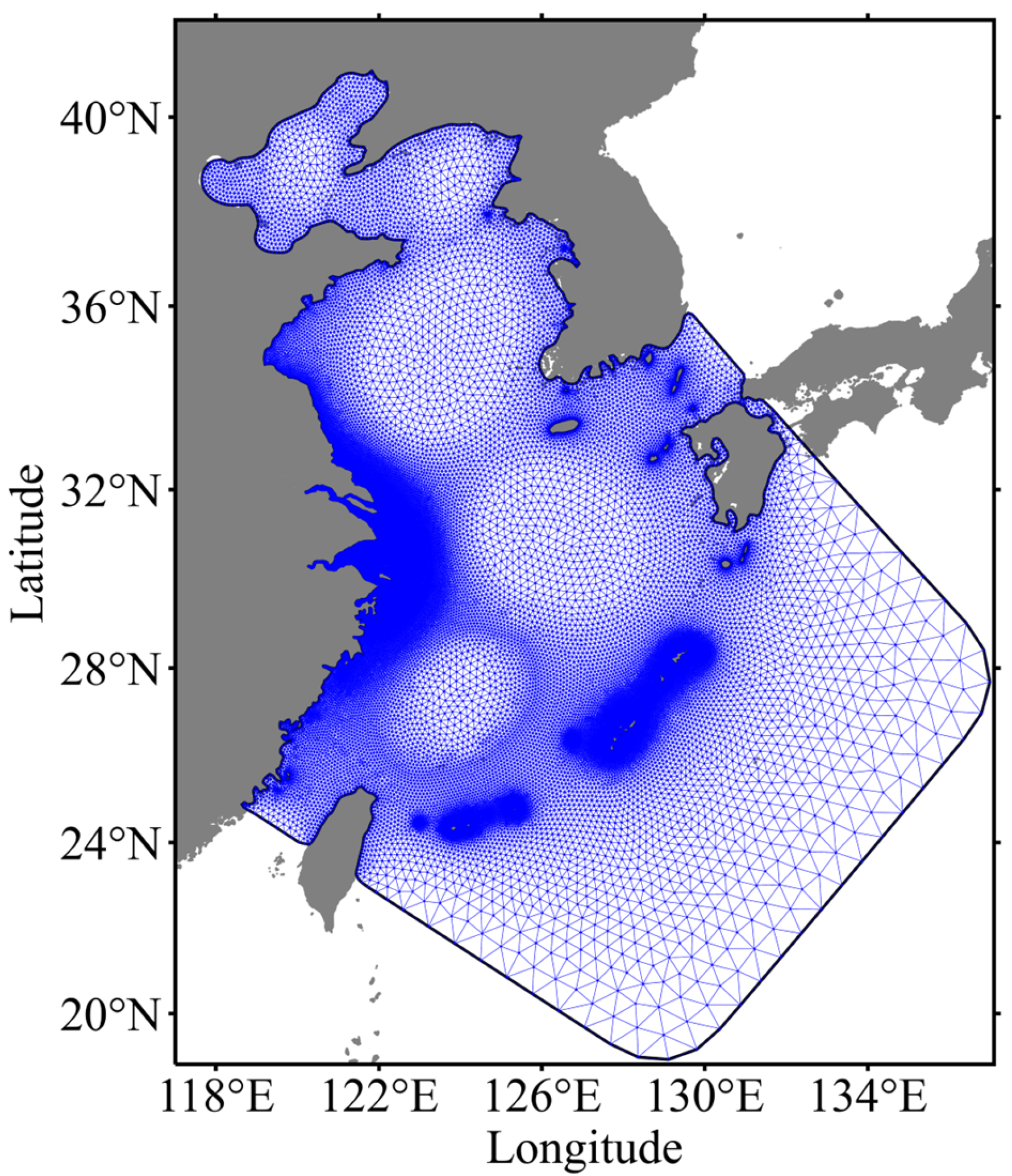
Figure 3.
Scatter density plots of modeled Hs forced by GFS analysis against satellite along-track measurements: (a) Jason-3, (b) Sentinel-3A, and (c) Sentinel-3B. The quantile-quantile (Q-Q) plot is superimposed to show the overall bias in distribution (green). The black, blue and dashed red lines indicate the perfect fit line, and the regression lines according to the regression model y = kx and y = kx + b, respectively.

Figure 4.
Comparisons of time series between model simulated and observed Hs at (a) HU01, (b) HU04, and (c) HU02. The grey lines denote observations, and the red lines represent the simulations forced by GFS analysis wind.
Figure 4.
Comparisons of time series between model simulated and observed Hs at (a) HU01, (b) HU04, and (c) HU02. The grey lines denote observations, and the red lines represent the simulations forced by GFS analysis wind.
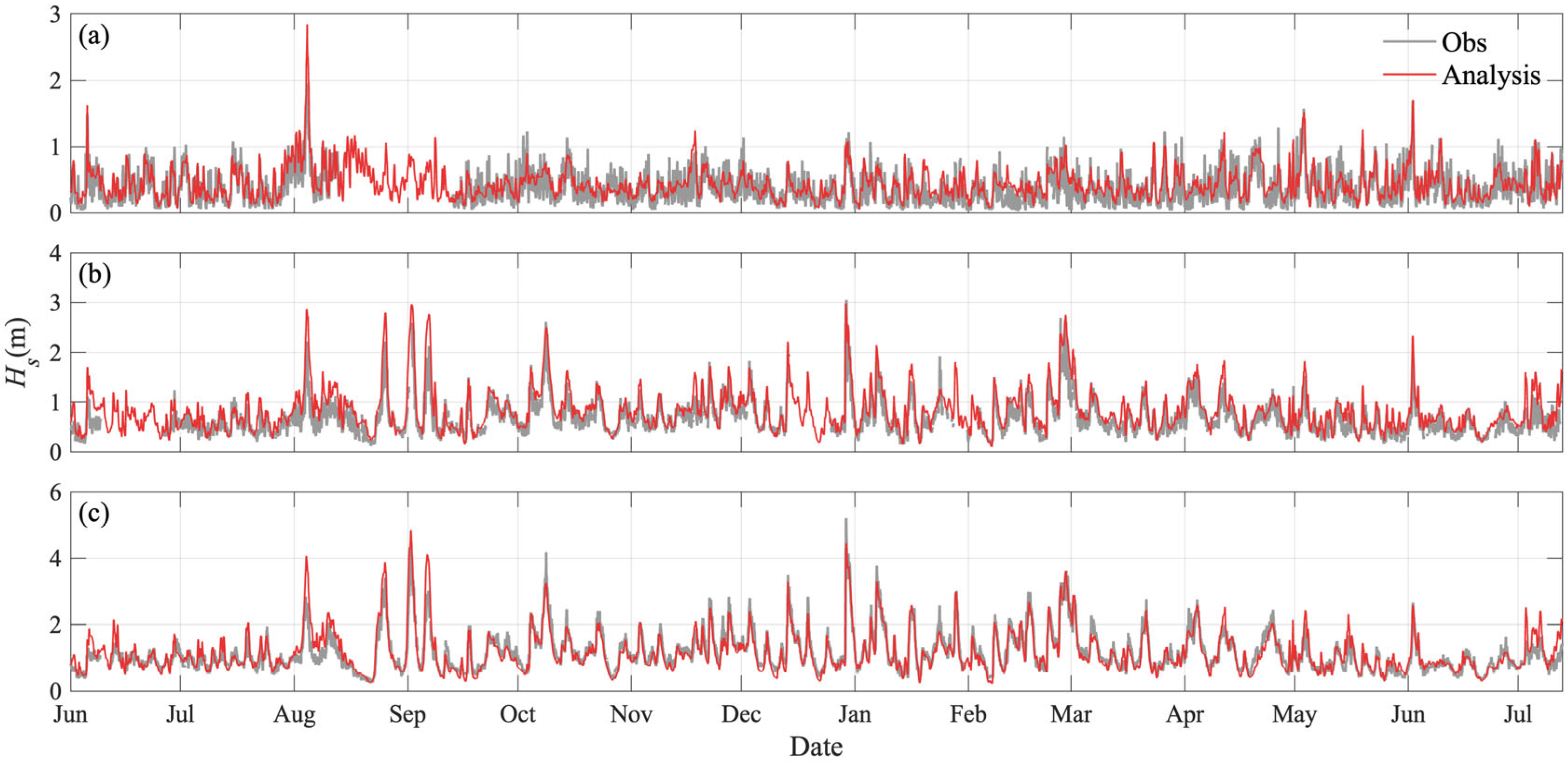
Figure 5.
Seasonal mean wave fields from June 2020 to May 2021: (a) summer, (b) fall, (c) winter, and (d) spring. The black vectors denote the mean wave direction.
Figure 5.
Seasonal mean wave fields from June 2020 to May 2021: (a) summer, (b) fall, (c) winter, and (d) spring. The black vectors denote the mean wave direction.
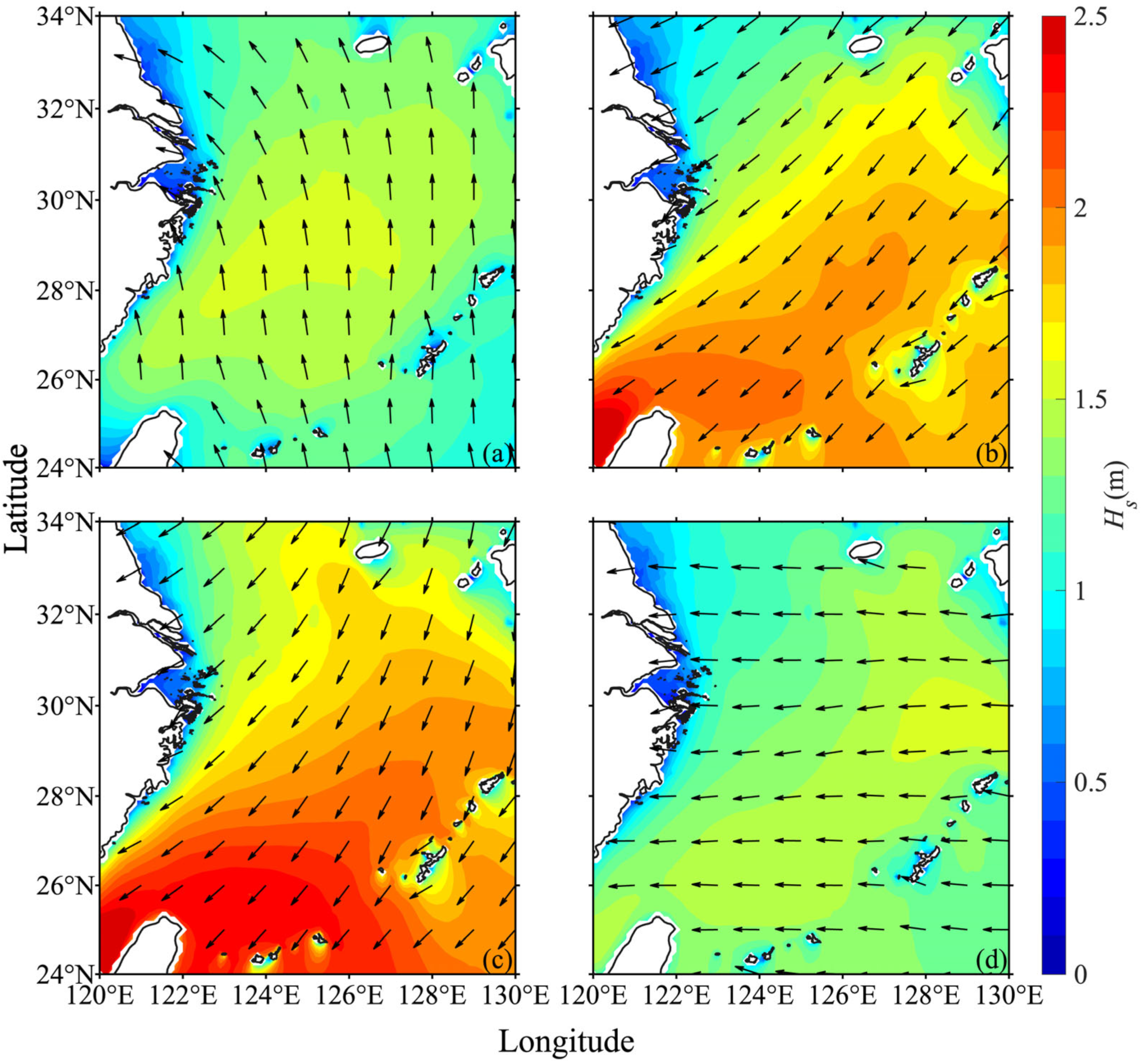
Figure 6.
Direction frequency of wind (left column) and wave (right column) in (a,b) summer, (c,d) fall, (e,f) winter, and (g,h) spring from June 2020 to May 2021 over the ECS shelf (28°–34°N, 120°–128°E). Sectors indicate the wave directions, or the directions wind vectors are directed towards. Colors are the wind speed and the Hs, respectively.
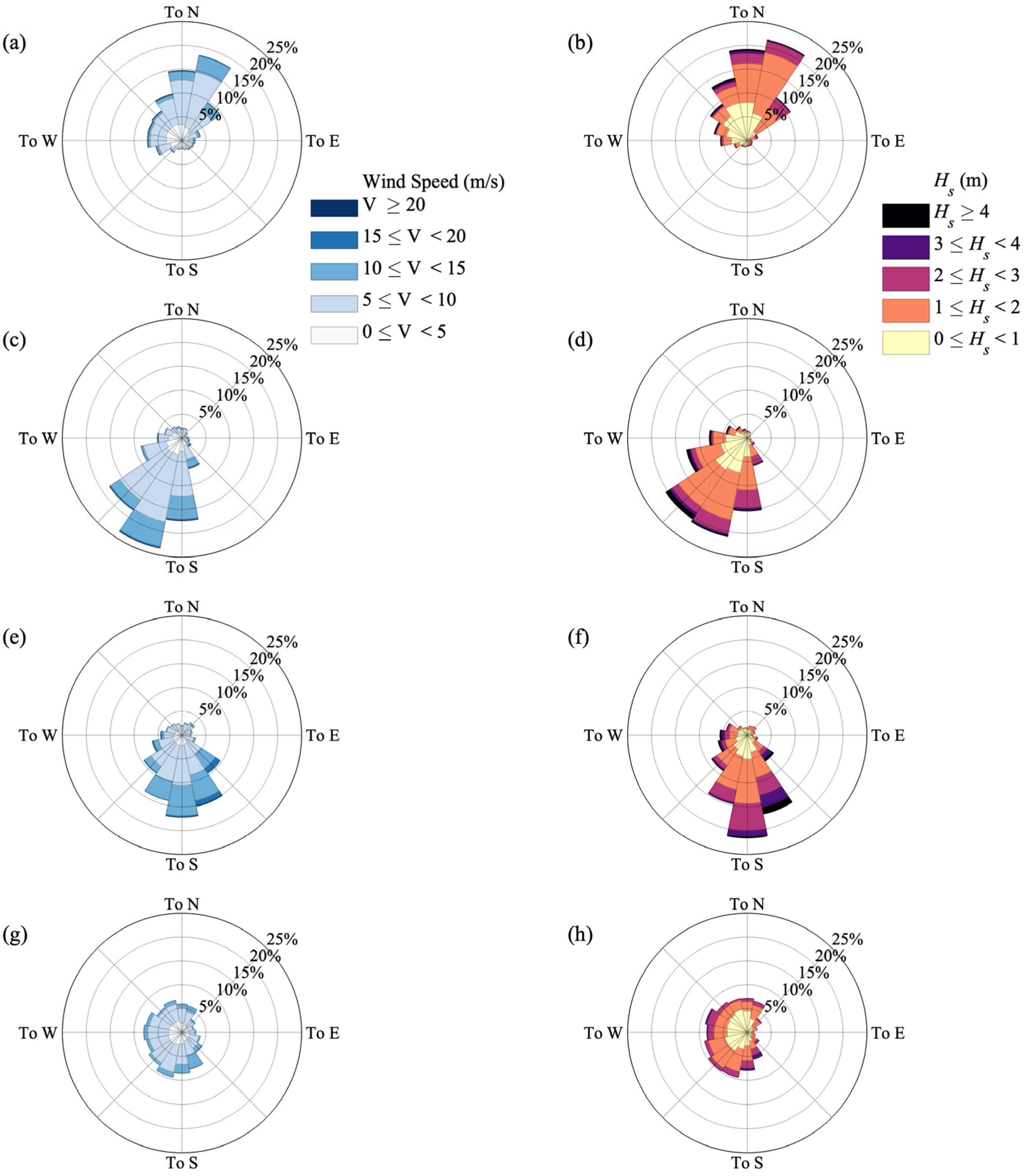
Figure 7.
Monthly mean (a) wind speed, (b) Hs, (c) Tm, and (d) wave direction at HU02 during June 2020 to June 2021. Solid dots show the monthly mean, and vertical bars show ± standard deviation for that month.
Figure 7.
Monthly mean (a) wind speed, (b) Hs, (c) Tm, and (d) wave direction at HU02 during June 2020 to June 2021. Solid dots show the monthly mean, and vertical bars show ± standard deviation for that month.
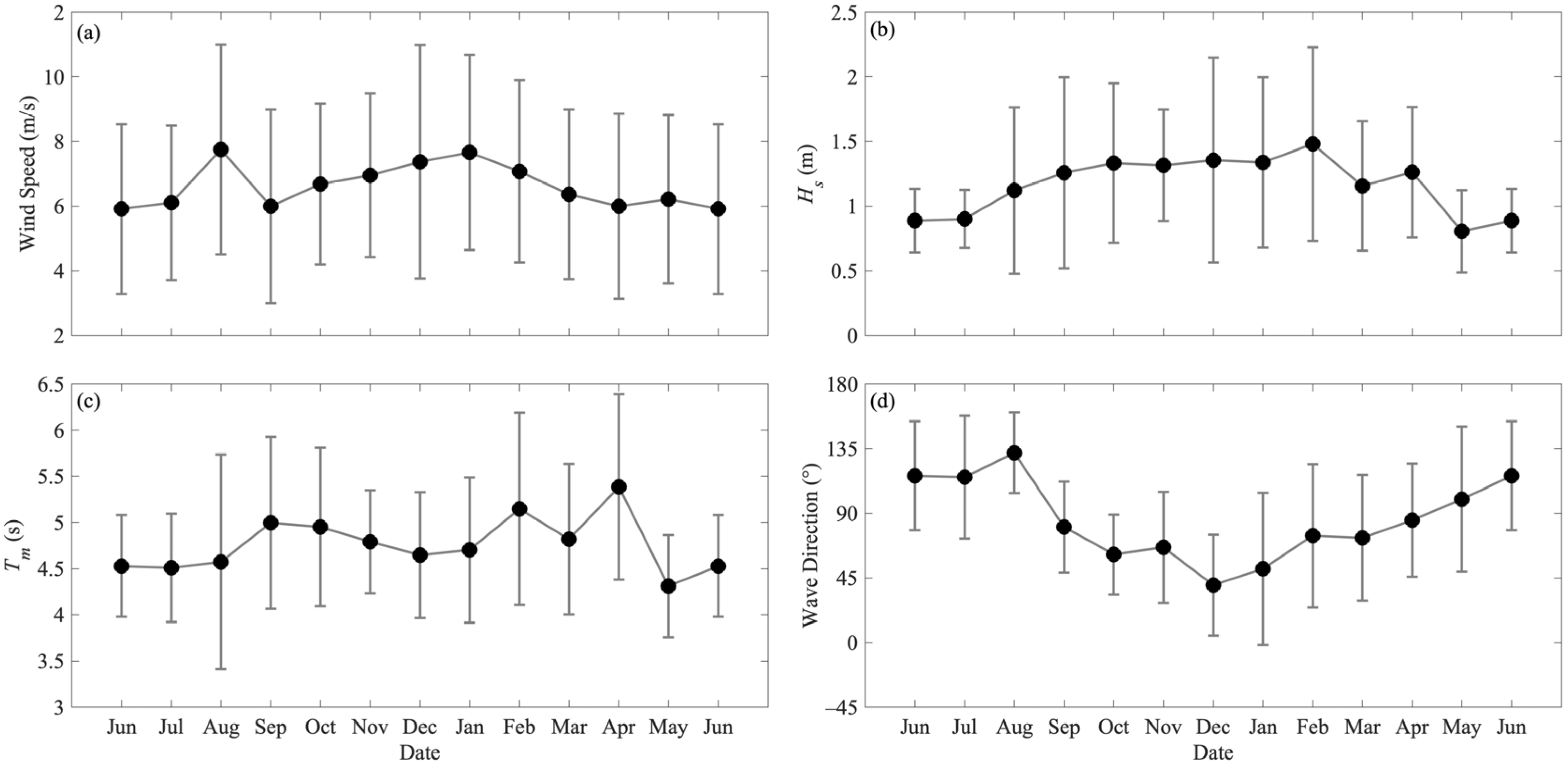
Figure 8.
Direction frequency of Hs (left column) and Tm (right column) observed at HU02 at (a,b) summer, (c,d) fall, (e,f) winter, and (g,h) spring from June 2020 to May 2021. Sectors indicate the wave directions. Colors are the Hs and Tm, respectively.
Figure 8.
Direction frequency of Hs (left column) and Tm (right column) observed at HU02 at (a,b) summer, (c,d) fall, (e,f) winter, and (g,h) spring from June 2020 to May 2021. Sectors indicate the wave directions. Colors are the Hs and Tm, respectively.
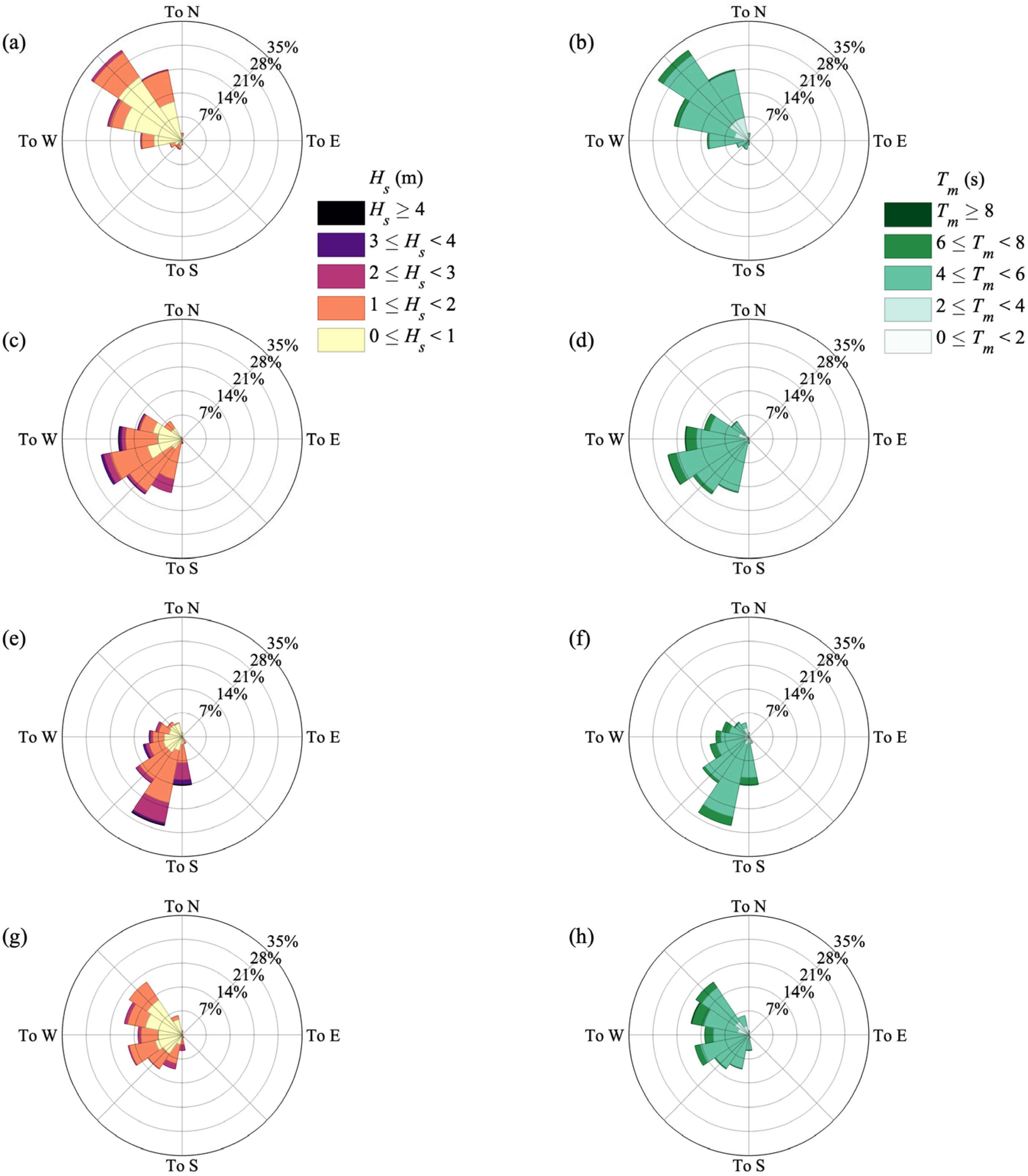
Figure 9.
Time series of observed and simulated Hs (black lines and red dots, respectively) and GFS wind analysis (blue lines) at (a,b) HU01, (c,d) HU04, and (e,f) HU02 station during the typhoon Maysak (left column) and the New Year’s Eve cold weather event at the end of 2020 (right column).
Figure 9.
Time series of observed and simulated Hs (black lines and red dots, respectively) and GFS wind analysis (blue lines) at (a,b) HU01, (c,d) HU04, and (e,f) HU02 station during the typhoon Maysak (left column) and the New Year’s Eve cold weather event at the end of 2020 (right column).
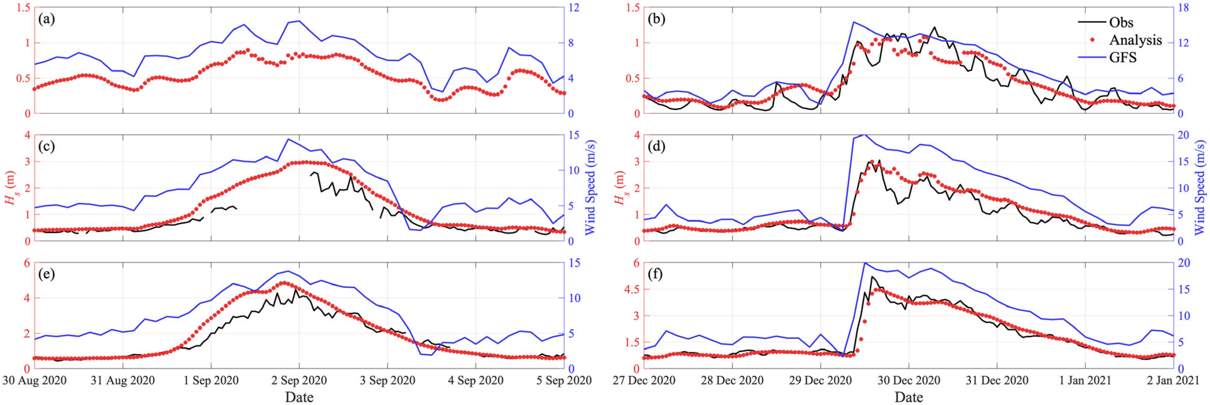
Figure 10.
Time series of observed wave direction (black arrows) (a,b) and peak period (black lines) (c,d) at HU02 station during the typhoon Maysak (left column) and the New Year’s Eve cold weather event at the end of 2020 (right column).
Figure 10.
Time series of observed wave direction (black arrows) (a,b) and peak period (black lines) (c,d) at HU02 station during the typhoon Maysak (left column) and the New Year’s Eve cold weather event at the end of 2020 (right column).

Figure 11.
Scatter density plots of buoy observed Hs against wave forecasts at 24 h, 48 h, and 72 h horizons at (a,d,g) HU01, (b,e,h) HU04, and (c,f,i) HU02. The quantile-quantile (Q-Q) plots are superimposed to show the overall bias in distribution (green). The black, blue and dashed red lines indicate the perfect fit line, and the regression lines according to the regression model y = kx and y = kx + b, respectively.
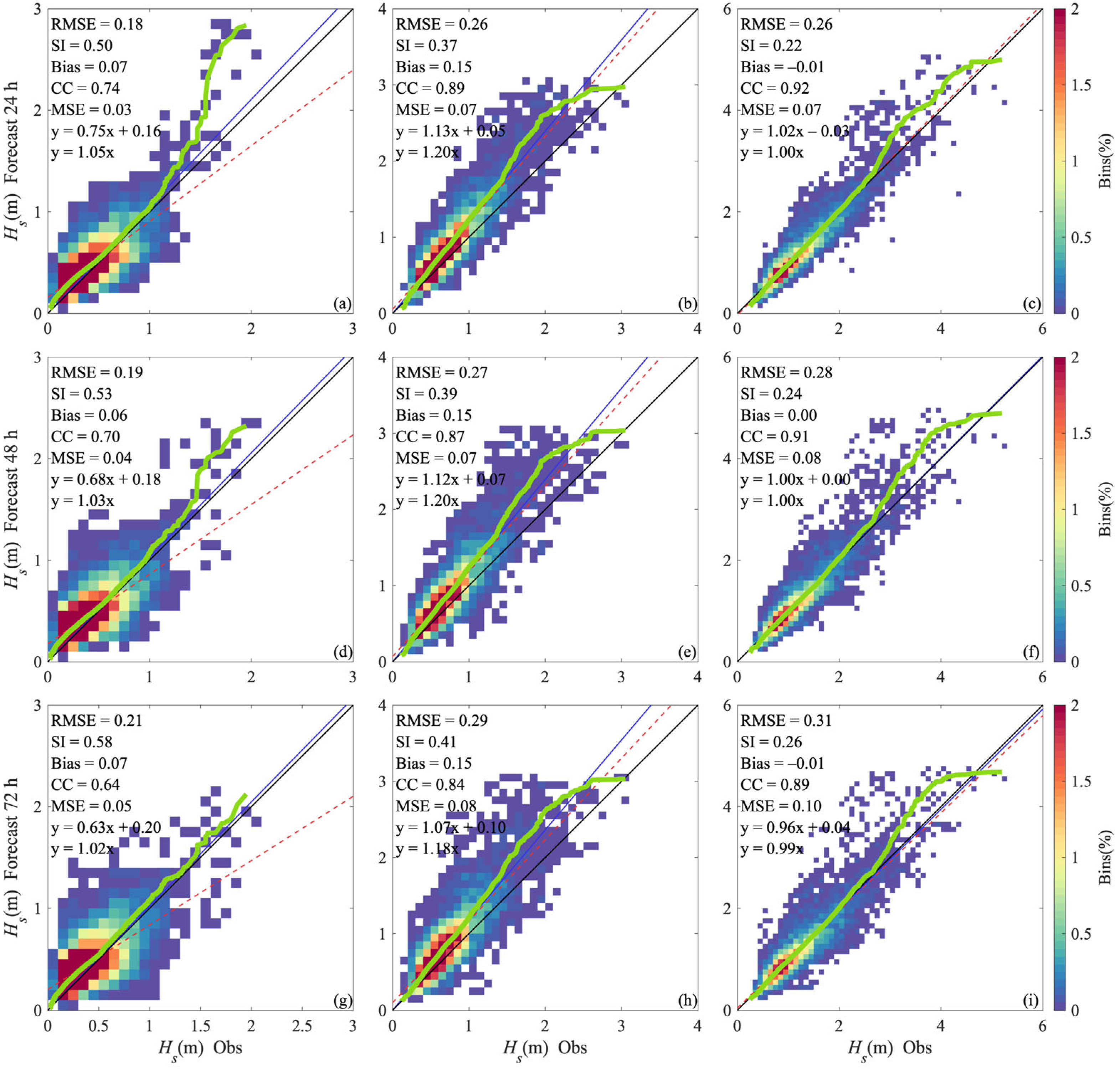
Figure 12.
Taylor diagram showing the difference between observed Hs and forecasts over different horizons at three buoy sites. The radial distance from the origin is proportional to the standard deviation of the reference. The RMSD between the test and the reference field is proportional to their distance apart. The correlation between the two fields is given by the azimuthal position of the test field.

Figure 13.
Scatter density plots of wave forecast at 24 h horizon against buoy observations in (a) summer, (b) fall, (c) winter, and (d) spring at HU02. The quantile–quantile (Q-Q) plots are superimposed to show the overall bias in distribution (green). The black, blue and dashed red lines indicate the perfect fit line, and the regression lines according to the regression model y = kx and y = kx + b, respectively.

Figure 14.
Altimeter–model bias as a function of the altimeter observed Hs for Jason-3, Sentinel-3A, and Sentinel-3B.
Figure 14.
Altimeter–model bias as a function of the altimeter observed Hs for Jason-3, Sentinel-3A, and Sentinel-3B.


Table 1.
Information of wave buoy sites around the Changjiang River Estuary.
| Buoy | Location | Buoy Type | Data Duration | Depth (m) |
|---|---|---|---|---|
| HU01 | (121.55°E, 30.75°N) | Triaxys | 1 June 2020–13 July 2021 | 9.25 |
| HU02 | (122.81°E, 30.97°N) | Triaxys | 1 June 2020–13 July 2021 | 27.88 |
| HU04 | (122.30°E, 30.97°N) | Triaxys | 1 June 2020–13 July 2021 | 10.38 |
Table 2.
Statistical parameters and the relative proportions of Theil decompositions of wave analysis versus buoy observations at three wave buoys.
Table 2.
Statistical parameters and the relative proportions of Theil decompositions of wave analysis versus buoy observations at three wave buoys.
| Station | RMSE (m) | SI | Bias (m) | CC | MSE (m2) | Theil Decomposition | ||
|---|---|---|---|---|---|---|---|---|
| Bias | Variance | Noise | ||||||
| HU01 | 0.18 | 0.50 | 0.07 | 0.75 | 0.03 | 13.38% | 0.02% | 86.6% |
| HU04 | 0.26 | 0.39 | 0.16 | 0.89 | 0.07 | 38.04% | 13.01% | 48.94% |
| HU02 | 0.26 | 0.23 | 0.02 | 0.91 | 0.07 | 0.52% | 3.9% | 95.59% |
Table 3.
Statistical parameters and the relative proportions of Theil decompositions of observed wind at Jiu-Duan-Sha versus forecast wind at 24 h, 48 h, and 72 h horizons.
Table 3.
Statistical parameters and the relative proportions of Theil decompositions of observed wind at Jiu-Duan-Sha versus forecast wind at 24 h, 48 h, and 72 h horizons.
| Wind | RMSE (m/s) | SI | Bias (m/s) | CC | MSE (m2/s2) | Theil Decomposition | ||
|---|---|---|---|---|---|---|---|---|
| Bias | Variance | Noise | ||||||
| 24 h forecast | 2.00 | 0.41 | 1.00 | 0.74 | 4.02 | 25.02% | 1.60% | 73.38% |
| 48 h forecast | 2.10 | 0.43 | 0.96 | 0.69 | 4.43 | 20.86% | 1.63% | 77.51% |
| 72 h forecast | 2.27 | 0.47 | 0.97 | 0.63 | 5.16 | 18.42% | 1.28% | 80.30% |
Table 4.
The relative proportions of Theil MSE decompositions for 24 h, 48 h, and 72 h forecasts versus buoy observations at three wave buoys.
Table 4.
The relative proportions of Theil MSE decompositions for 24 h, 48 h, and 72 h forecasts versus buoy observations at three wave buoys.
| Station | Forecast Horizon | Bias | Variance | Noise |
|---|---|---|---|---|
| HU01 | 24 h | 13.41% | 0.00% | 86.59% |
| 48 h | 11.00% | 0.08% | 88.92% | |
| 72 h | 10.57% | 0.02% | 89.41% | |
| HU04 | 24 h | 33.41% | 14.16% | 52.43% |
| 48 h | 30.50% | 13.59% | 55.91% | |
| 72 h | 25.99% | 11.44% | 62.57% | |
| HU02 | 24 h | 0.06% | 6.15% | 93.78% |
| 48 h | 0.02% | 5.06% | 94.91% | |
| 72 h | 0.05% | 2.54% | 97.41% |
Disclaimer/Publisher’s Note: The statements, opinions and data contained in all publications are solely those of the individual author(s) and contributor(s) and not of MDPI and/or the editor(s). MDPI and/or the editor(s) disclaim responsibility for any injury to people or property resulting from any ideas, methods, instructions or products referred to in the content. |
© 2023 by the authors. Licensee MDPI, Basel, Switzerland. This article is an open access article distributed under the terms and conditions of the Creative Commons Attribution (CC BY) license (https://creativecommons.org/licenses/by/4.0/).
Share and Cite
MDPI and ACS Style
Jiang, Y.; Rong, Z.; Li, Y.; Li, C.; Meng, X. Toward a High-Resolution Wave Forecasting System for the Changjiang River Estuary. Remote Sens. 2023, 15, 3581. https://doi.org/10.3390/rs15143581
AMA Style
Jiang Y, Rong Z, Li Y, Li C, Meng X. Toward a High-Resolution Wave Forecasting System for the Changjiang River Estuary. Remote Sensing. 2023; 15(14):3581. https://doi.org/10.3390/rs15143581
Chicago/Turabian StyleJiang, Yan, Zengrui Rong, Yiguo Li, Cheng Li, and Xin Meng. 2023. "Toward a High-Resolution Wave Forecasting System for the Changjiang River Estuary" Remote Sensing 15, no. 14: 3581. https://doi.org/10.3390/rs15143581
Note that from the first issue of 2016, this journal uses article numbers instead of page numbers. See further details here.