
An Effective Method of Infrared Maritime Target Enhancement and Detection with Multiple Maritime Scene

1
School of Mechanical and Electrical Engineering, Guilin University of Electronic Technology, Guilin 541004, China
2
School of Electronics and Information, Wuzhou University, Wuzhou 543002, China
3
College of Communication and Information Technology, Xi’an University of Science and Technology, Xi’an 710699, China
4
School of Information Engineering, Henan Institute of Science and Technology, Xinxiang 453003, China
*
Author to whom correspondence should be addressed.
Remote Sens. 2023, 15(14), 3623; https://doi.org/10.3390/rs15143623
Submission received: 5 May 2023
/
Revised: 15 July 2023
/
Accepted: 17 July 2023
/
Published: 20 July 2023
(This article belongs to the Special Issue Remote Sensing in Intelligent Maritime Research)
Abstract
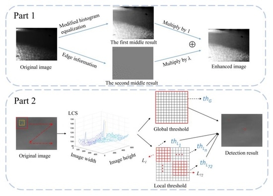
:Aiming at maritime infrared target detection with low contrast influenced by maritime clutter and illumination, this paper proposes a Modified Histogram Equalization with Edge Fusion (MHEEF) pre-processing algorithm in backlight maritime scenes and establishes Local-Contrast Saliency Models with Double Scale and Modes (LCMDSM) for detecting a target with the properties of positive and negative contrast. We propose a local-contrast saliency mathematical model with double modes in the extension of only one mode. Then, the big scale and small scale are combined into one Target Detection Unit (TDU), which can approach the “from bottom to up” mechanism of the Visual Attention Model (VAM) better and identify the target with a suitable size, approaching the target’s actual shape. In the experimental results and analysis, clutter, foggy, backlight, and dim maritime scenes are chosen to verify the effectiveness of the target detection algorithm. From the enhancement result, the LCMDSM algorithm can achieve a Detection Rate (DR) with a value of 98.26% under each maritime scene on the average level and can be used in real-time detection with low computational cost.
1. Introduction
Infrared (IR) imaging technology has been widely used in target search and maritime navigation [1], maritime navigation [2], and maritime environmental variation [3,4]. IR imaging data can reflect object distance information and target shape information within the maritime background in two dimensions. However, multiple factors, such as complex maritime background and changing illumination, can often cause the infrared maritime target to disappear in the background clutter [5,6,7]. According to our infrared imaging experiment and image analysis, in most cases, the target presents the property of positive contrast when its gray value is higher than the average gray value of its surrounding background. However, in some special cases, the gray value of the target is lower than the average gray value of its surrounding background, which can be described by the property of negative contrast, and the target easily disappears in the backlight maritime scene. Hence, an effective pre-processing algorithm needs to be proposed to enhance infrared small targets under backlight maritime scenes. The maritime scene discussed in this paper includes four main categories: strong winds, heavy fog, long-distance aerial photography from a bird’s-eye view, and backlight conditions. It does not include severe weather conditions.
Many image enhancement techniques based on Histogram Equalization (HE) [8] have been developed to deal with IR images with low quality, which can highlight a target from the background and change its illumination to some extent [9,10]. For example, the classical Histogram Equalization (HE) algorithm changes the illumination influence and improves the image contrast by equalizing the Probability Density Function (PDF) of the image gray value distribution to some extent. The Minimum Mean Brightness Error Bi-Histogram Equalization (MMBEBHE) [11] algorithm utilizes two sub-histograms equalization algorithms to keep the mean brightness constant. The Edge-Based Texture Histogram Equalization (ETHE) [12] algorithm equalizes the edge part’s histogram and uses it as the transform function in the total image, which can enhance image details. The Contrast-Accumulated Histogram Equalization (CACHE) [13] algorithm incorporates the information around pixels into the density estimation of HE to avoid strong noise coming from the background and loss of image details. However, some parts of the image may lose detail, and its effectiveness in image detail enhancement is limited when the image contains both over-dark and over-bright regions. The Recursive Separated and Weighted Histogram Equalization (RSWHE) [14] algorithm splits an input histogram into more than two sub-histograms recursively based on the mean or median of the sub-image to modify the sub-histogram by a normalized power-law function and then equalizes the weighted sub-histogram. It can keep remarkable brightness and enhances the contrast but easily produces artifacts [15,16] in the image.
Generally speaking, IR target recognition approaches can be divided into three categories [17]: (1) background consistency-based model, (2) VAM-based model, and (3) low-rank and sparse decomposition-based model.
Background consistency-based methods first estimate the original image background using a filter; then, they enhance and extract the target from the background [18]. Common filters used include the Top-Hat filter [19], the max-mean/max-median filter [20], and the median subtraction filter [21]. In addition, Jia et al. [22] proposed a Saliency-Guided Double-Stage Particle Filter (SGDS-PF) consisting of a searching Particle Filter (PF) and tracking PF, which achieved high tracking precision even under intensive noise. Tang et al. [23] used a dilate filter to increase the characteristic information of the suspected target, which was able to detect the suspected target easily, and the time complexity was very low. However, if the target disappears in the background in an infrared image, this algorithm cannot be valid. Chan et al. [24] proposed the Background Subtraction (BS) method, and it was applied to detect visible targets. However, it is not fit for small IR targets and has some problems detecting targets surrounded by a complex background. Furthermore, infrared images are often complicated and contain a lot of random clutter. Therefore, the background consistency-based model is very susceptible to clutter, noise, and other complex backgrounds.
A common VAM-based model is the Local-Contrast Method (LCM) [25]. The first stage of the LCM algorithm is to establish the Local-Contrast Saliency Map (LCSM) by a window structure and quantify it by a reasonable mathematical model. The second stage is the threshold selection for the suspected target from the entire image’s LCSM. Finally, the algorithm identifies the suspected target area. There have also been many improved algorithms based on LCM in recent years, such as Multi-Scale Patch-Based Contrast Measure (MPCM) [26], Weighted Three-Layer Window Local-Contrast Method (WTLLCM) [27], Integrated Target Saliency Measure (ITSM) [28], Relative Local Contrast Measure (RLCM) [29], Multi-Directional Gradient Improved Double-Layer Local-Contrast Method (MGIDLCM) [30], and Maritime Noise Prior (MNP) [31]. The main principle of the MPCM is to calculate the grayscale mean difference in eight different directions of surrounding patches, which can generate the dissimilarity measure between surrounding patches and form a multi-scale patch-based contrast measure. As a result, it can detect bright and dark targets. If the target’s size is smaller than the detecting patch, the algorithm may fail, and the multiple scale is not suitable for different target sizes. The WTLLCM performs hierarchical gradient kernel filtering on the image to calculate the local contrast, then proposes a region intensity level algorithm to suppress the background, and finally detects target by adaptive threshold. It uses single-scale windows instead of multi-scale windows to complete multi-scale target detection, which can reduce the calculation complexity. However, the target pixels are easily lost during the process. The idea of ITSM is to utilize a simple image filter, and two middle filter results are multiplied to produce the final detection result. However, it can only detect the positive contrast target without measuring Local Contrast Saliency (LCS) with the property of positive contrast and negative contrast. Both the concept of relative local contrast and a relative mathematical model are developed in RLCM. As the image contains four different regions such as the real target region, the region surrounded by pixel-sized noises with high brightness, region with double background edges, and the pure background region, these four regions’ relative local contrast are calculated and studied, which presents obvious differences in the IR image. However, RLCM cannot be applied in detecting negative-contrast property targets. MGIDLCM mainly establishes meticulous LCS models, including the concept of multi-layer contrast differences between internal and external neighborhoods and the fusion of gradient information with different directions. As a result, this algorithm can improve the DR of a true target but fails in fitting for a true target’s size. As for the MNP algorithm, complex maritime conditions affect the target’s detection; for example, the false alarm rate may be increased. Some methods based on average absolute gray difference (AAGD) [32] also utilize the similar methodology of LCM, such as ADDGD [33] and AMAD [34]. ADDGD forms the deep insight into the mathematical model establishment for the suspected target with a high DR in the infrared image. This algorithm has special effectiveness for the dim infrared target. ADMD produces the saliency map by the absolute directional mean difference to detect the target. Although this mechanism can suppress the noise, the threshold for target is difficult for selection.
The low-rank and sparse decomposition-based model pays more attention to the essence of the infrared images and uses the attributes of background and target. Gao et al. [35] discovered that the infrared image background possesses the property of non-local self-correlation, and the number of pixels in the target area is much less than the number of pixels in the original image. They treat the patch image of the background as a low-rank matrix and the block image of the target as a sparse matrix, transforming the small target detection into an optimization problem with low-rank decomposition. Inspired by this method, various models for the decomposition of low-rank sparse matrices have been proposed, such as NRAM [36], NTFRA [37], and ANLPT [38]. NRAM proposes the new concept of target detection. The model of the target area is established by a group of objective functions and constrained conditions. Although the algorithm has many iteration times, the detection result has good performance. NTFRA algorithms’ principle is similar with the NRAM’s. It can extract the local region’s property and obtain the tensor matrix with three dimensions; then, the target can be decomposed by some iterative formula. This algorithm can suppress the clutter effectively, but the time complexity is high. ANLPT uses the principle of low-rank sparse tensor decomposition to detect the infrared small target. The rank of the patch in an image can reflect the difference of the target and background. However, this algorithm’s complexity may be high and not fit for different target sizes.
The main contributions of this article are summarized as follows.
- (1)
- Proposing the effective image pre-processing algorithm for the backlight maritime scene, the pre-processing result’s output can be used as the input data source of the image target’s detection algorithm, which can improve the DR of image’s infrared maritime true target.
- (2)
- Study the mathematical model of LCS for the suspected target with the property of both positive contrast and negative contrast. By contrast, the conventional LCM algorithm is only fit for detecting the target with the property of positive contrast. Moreover, we establish the suspected target detection mechanism with the global and local threshold selection strategy.
- (3)
- Establish the structure of image target detection unit with double scale, which approaches the “from bottom to top” mechanism of VAM. The maximum saliency map of the integrated two scales in the TDU can determine the approximate target area, and the source scale from the maximum saliency map can locate the target with high precision. Moreover, it is highly noted that the detection algorithm based on LCS establishment with double scale be able to have more opportunities to find the true targets, and the concerned parameters can be selected adaptively according to the size definition of a small target from SPIE.
2. Materials and Methods
2.1. Equipment and Image Acquisition Manner for Infrared Maritime Target
Figure 1a illustrates the integrated maritime imaging equipment which contains an infrared medium-wave camera, visible camera, and infrared long-wave camera. This equipment has a maximum target capture distance of 20 km for a duration of two hours and acquires an image dataset of 640 × 512 pixels. So, the data processing volume of the proposed algorithm is approximately from 320,000 to 330,000 pixels. Both the infrared medium-wave camera and the infrared long-wave camera have the imaging ability of high distance, fog-penetrability, and day-night working, so the infrared camera is widely used in the maritime search and rescue. Figure 1b is experimental imaging spot by the fixed location at Marina Bay Plaza in Dalian on 18 March 2022. After the progress of infrared image restructured by the internal equipment, the digital infrared maritime image can be acquired and processed.
2.2. The Proposed Pre-Processing MHEEF Algorithm
The proposed pre-processing algorithm needs to change the backlight illumination condition, highlight the target region that might be obscured by a strong background, and enhance the target local contrast while suppressing the background variation.
2.2.1. Obtain the New Histogram and New Histogram Equalization
The maritime backlight scene is shown in Figure 2. The gray value of the background tends to be in a larger proportion and varies on a smaller gray scale, as shown in Figure 3a. To obtain the enhancement result, we need to modify the proportion of pixels in the original histogram for the reason that the proportion in the histogram has positive correlation with the enhancement rate [39] and then normalize it.
Figure 3b illustrates the modified method for the new histogram, which contains peak value detection, modification of proportion of pixel, and proportion normalization. The first stage is finding the maximum proportion of pixels called Pmax, and the main procedure in the second stage is the proportion limit according to Pmax. The main mathematical model can be expressed as Equation (1):
where is the proportion of original histogram, is the maximum proportion after modification, is the proportion of pixels after modification, and v is proportional parameter, which generally has a range of [1/3, 2/3]. This paper choses the value of 2/5.
The third stage is normalization of proportion value which can be expressed as Equation (2):
where is proportion of the new histogram after normalization.
The progress of gray value transformation for the new histogram can be expressed as .
2.2.2. Edge Information Quantification and Fusion into the First Middle Result
The previous research [40] shows that HE cannot reflect the gray variation between the central pixel and its neighbor pixels. Hence, the modified histogram equalization result with effective edge information fusion can be used to enhance the target’s local details and add the high-frequency component.
In order to quantize the image’s edge information, the second order difference operator for with 8 neighbor pixels in the image is used, and it can be expressed as Equation (4):
where means the edge information of pixel coordinate in the original image.
The filter of edge information quantification is shown in Figure 4a, which can traverse by each pixel in the image to obtain the filtering result. Figure 4b illustrates the filtering result of Figure 2a using the filtered element from Figure 4a. To avoid the image edge information appearing excessively dark, the result is initially magnified by a factor of five times and then increased by 128. This process primarily enhances the local target texture and improves local contrast for subsequent detection. The edge quantification can be expressed as , where is the second middle result of original image .
2.2.3. Final Enhancement Result of Pre-Processing Algorithm
The first middle result for Figure 2a is shown in Figure 5a, in which can be seen that the histogram equalization by maximum proportion limit algorithm improves the image’s illumination condition on the basis and highlights the maritime IR target from the background. However, the first middle result fails in local detail improvement.
Then, integrating Y1 with Y2 in the format of “1 + λ”, the mathematical model can be expressed as Equation (5):
where Y means the final enhancement result of MHEEF algorithm, and λ means the gain factor of edge information. Generally, the larger the value of λ is, the more the details in IR image improves. At the same time, it will generate more noise easily. Our previous experiments show that λ can be chosen by the value range of 1~2. Then, λ = 1 is chosen for result’s illustration.
2.3. The Proposed LCMDSM Detection Algorithm
In this section, we discuss the three significant procedures in the LCMDSM algorithm. The first one is to establish the structure of TDU with double scale, which combines the big and small scale and the central point of the two scales traverse in the entire image. The second one is to establish the mathematical model of LCSM for suspected target with the property of both positive and negative contrast. Then, integrate the LCM with double scale, obtain the maximum result of LCM, and find the source scale for the maximum result which can approach the VAM mechanism of “from bottom to top”. At last, the global and local threshold selection for detecting the suspected target region in the entire image are discussed.
2.3.1. The Structure of TDU with Double Scale
As shown in Figure 7, the rectangle region drawn in the red full line outlines the TDU (the same with the big scale’s outline in the TDU), which includes one target region with big scale drawn in the blue full line and nine background regions with the same size. The red line means the background area with double scale, and the blue line means the target area with double scale in Figure 7. At the same time, each target region with big scale can divide into nine target regions with small scale drawn in the blue dummy line, correspondingly the nine background regions with small scale are surrounding with it. The size of the global TDU is w2 × w2, in which the size of target named by T with big scale is w1 × w1. Similarly, the size of background named by B1, B2, …, B8 is also w1 × w1. The LCS with big scale, denoted by Cn, can be calculated by measuring the dissimilarity between the T block and the B1, B2, …B9 blocks (n denotes the serial number of the TDU in the image). With the same structure, the target with small scale named t1 has the size of w0 × w0, and the background regions surrounding the target t1 are named by , respectively. The target with small scale named by t1,t2, …, t9 can also produce the LCS called . The central point named (x0, y0) is located in the center of both region T and t5, which can traverse in the entire image and produce the LCS with the integrated double scale under the proposed algorithm. What is more, according to the definition of small target by SPIE, the number of pixels in the small target area is less than 0.15% of the image’s entire pixels. Thus, if the image has a width value of W and a height value of H, the square of target area is less than 0.15% × W × H. As for the size of TDU, the value of w2 can be chosen by a integer number derived from times by three, which also needs to be less than . w1 can be chosen by one-third of w2, and w0 can be chosen by one-third of w1, so the parameter initialization of TDU is set automatically, which can be adaptive with different image’s size.
Figure 8 shows the moving direction of targets with big and small scale in the image. The red full arrow shows the moving direction of the TGU, while the blue dummy arrow represents the moving direction of target with small scale. The red solid rectangle means the background area with big scale; the blue solid rectangle means the target region with big scale; and the blue dashed rectangle means the target region with small scale.
As for the program implementation, firstly, the point centered by TDU traverses in the entire image, which can be put as a main cycle in the image; then, the target region T and the background region B with big scale are found, and can be calculated. Meanwhile, the central point for t1, t2, …, t9 can be easily calculated by central point . The LCS with small scale, represented by , can be easily calculated from the confirmed target area and background area with small scale. From the opportunities for target detection, TDU with only one scale searches for the suspected target with only once such as LCM algorithm, whereas TDU with double scale can search for the suspected target with ten times, which can improve a DR.
2.3.2. The Mathematical Model for Target Detection with Positive Contrast and Negative Contrast
The IR target presents the property of positive contrast or negative contrast in the IR image. In order to better measure its LCS, the mathematical models for target detection with positive contrast and negative contrast are different. If the target has the characteristic with positive contrast, it can be described by Equation (6); on the contrary, it can be described by Equation (7):
where is the nth LCS of TDU under the big scale, T and represent the target region and background region in the big scale, is the nth LCS of TDU in the small scale, and and represent the target region and background region in the small scale. The basic principle of Equation (6) is that the gray value of target region is higher than the surrounding background region on the average level, which can generate the dissimilarity measure correctly between them and outstand the saliency by the square arithmetic and so is the basic principle of Equation (7) for the negative target. Notably, the squaring operation in Equation (7) can amplify the target’s weak difference around the background.
In order to obtain the integrated result of LCS through double scale, the maximum pooling strategy is used, which can be expressed as Equation (8):
where is the final integrated result of the nth serial number that TDU has traversed. We can detect the target region by the proposed threshold selection strategy through in the following.
2.3.3. Threshold Selection Strategy for LCS and Target Rectangle Output
According to numerous previous research tests, the true target usually has a much larger value of than the average value of LCSM. Combined with statistical laws, the suspected target region which has a large value of LCSM dominates a very small proportion in the entire . Thus, the threshold selection strategy for finding suspected target regions can be expressed as Equation (9):
where is the global threshold of . is the average value of ; is the standard deviation of ; and k is a given proportion coefficient which can measure the distance between and the k times of . Correspondingly, the threshold selection strategy described as Equation (9) can be similarly used in the local region of . We can obtain the local threshold of by setting the size of 5 × 5 to format the local searching area in .
In our previous experiments, we observed that when the value of k is larger, the standard for detecting suspected targets becomes more strict, which can result in missing true targets that submerged into the maritime background. On the contrary, when k is smaller, the standard becomes looser, which can result in detecting more false targets in the background. Our experiments have shown that the usual range of k is between 2 and 5, and it can be chosen by 3 in the common case or in the optimal condition [41].
Figure 9 is the diagram of global threshold selection and local threshold selection from the matrix . The global matrix can produce the one global threshold named by when the element in has a larger value than which can be judged as the suspected target. In addition, each element in the can format the local searching region with the size of 5 × 5. The local searching region can produce the local threshold named by . If the value is larger than , the element can also be judged as the suspected target. In Figure 9, the number in LCSM of matrix represents the value of LCSM. The red rectangle in the Global threshold and Local threshold represents the global region and local region, respectively.
Figure 10 shows the diagram of target searching mechanism in LCMDSC, which can approach to the VAM criteria. The matrix is the “bottom”. The value of is based on which matrix it comes from and is equal to the inverse process of Equation (8). Positive and negative contrast are physical properties. The presence of a target with a gray scale higher or lower than the average gray scale of the background does not determine the contrast value as positive or negative. The contrast values calculated by Equations (6) and (7) are both positive. The number in means the combined LCS with double scale, and the number in means the LCS with small scale.
As discussed above, the pseudocode of Algorithm LCMDSM can be described as Table 1. From each process, it can be concluded that both the time complexity and space complexity of LCMDSM algorithm are when the original image has the scale of .
3. Results
3.1. The Contribution of the Pre-Processing MHEEF Algorithm
Figure 11 shows the 3D diagrams of LCSM of Figure 2a and its enhancement result from the MHEEF algorithm, where the red rectangle demonstrates the location of a suspected target’s region of Figure 2a in the 3D LCSM. Obviously, the LCS of the target region is improved after the pre-processing algorithm, which can detect the suspected targets easily.
Similarly, Figure 12 is the 3D diagrams of LCSM of Figure 2b and its enhancement result from the MHEEF algorithm, where the red rectangle demonstrates the location of a suspected target’s region of Figure 2b in the 3D LCSM., and it can be seen that the LCS of the suspected target region after the MHEEF algorithm is increasing more obviously than before. Therefore, the enhancement result of backlight maritime scene can be helpful for the target detection, which can be put as the effective input data for the detection algorithm such as our proposed LCMDSM algorithm.
3.2. The Objective Image Quality Assessment of Enhancement Result
In order to objectively assess the performance of the pre-processing algorithm, the Average Gradient (AG) and the Enhancement Measure by Entropy (EME) [42] are used to evaluate the original image and the enhancement result’s objective quality.
The AG reflects the richness of texture and details in the image. A higher value of AG indicates that an image has more details and texture, and its computing model can be expressed as Equation (10):
where is the gradient value of an image, and the gradient value of the current pixel in the ith row and the jth column of an image are calculated by the central difference measure.
The EME can reflect the average entropy of the local contrast in the image. In a common case, a higher value of EME indicates that an image has more contrast, and its computational model can be expressed as Equation (11):
where W and H are the width and height of the image, m and n are the width and height of the sub-blocks divided from the processed image, and and are the maximum value and minimum value in the sub-block which is located in the ith row and jth column of the image’s sub-block. operator represents the process of rounding down for a number.
In order to evaluate the proposed pre-processing algorithm fairly, HE, MMBEBHE, and ETHE algorithms are used for the comparison. Figure 13 and Figure 14 are the enhancement results of each algorithm for Figure 2a,b, respectively.
Table 2 is the AG and EME of original image and the enhancement results. It can be seen that the AG of the proposed algorithm improves at least twice as many times compared with the original image, and it is also the largest value of AG compared to other algorithms. Therefore, the proposed algorithm can highlight the image details efficiently. As for the EME assessment, the proposed algorithm achieves the best. Because the structure of EME calculating model is similar with the TDU’s [42], it can be deduced that the proposed MHEEF algorithm is beneficial for the target detection.
As for the objective quality assessment of the local target region, Background Suppression Factor (BSF), Signal-to-Clutter Ratios (SCR), and Local Contrast Gain (LCG) [43] are used to evaluate the target region’s quality. BSF represents the degree of noise or clutters suppression, which is demonstrated in Equation (12):
where and are the standard deviations of the image background in the original image and the result, respectively.
SCR is widely used to measure the difference between the target and its neighborhood, which can be expressed as Equation (13):
where is the average gray value of the targets, and and are the average and standard deviation of the background, respectively.
LCG can evaluate the dissimilarity between the target and its surrounding background region with respect to the result and original image, which can be expressed as Equation (14):
where CONr and CONo are the local contrast of the target in the enhancement result and original image, respectively.
Figure 15 shows the region division diagram for the target and its neighborhood region in Figure 2a,b, where the red rectangle indicates the obscured target region and the blue rectangle indicates the neighborhood region around the target.
Table 3 is the comparison of BSF, SCR, and LCG of the original image and the enhancement results, in which can be seen that the BSF, SCR, and LCG of the proposed pre-processing algorithm are the largest or the second largest of the compared algorithms. Therefore, it can be highly noted that the proposed MHEEF algorithm not only enhances the target region’s details but suppresses the maritime clutters, especially for the local small target’s region in an infrared image.
3.3. The Target Detection Results of LCMDSM Algorithm and Compared Algorithms
To validate the effectiveness of the proposed method, we compared it with seven other state-of-the-art unsupervised infrared small target detection algorithms, namely LIG [44], NRAM [36], ADDGD [33], ADMD [34], NTFRA [37], GCMDO [23], and ANLPT [38]. To avoid unfair comparison and assessment, we used four maritime datasets from integrated maritime imaging equipment to compare the target detection results of the LCMDSM algorithm with those of the other algorithms, and three representative images from each infrared maritime dataset were shown. The four figures below show the original image with ground truth and target detection results by using different detection algorithms. The blue rectangle region on the left side of each figure indicates the factual target region; the small red rectangle represents the detected target’s region by the proposed algorithm; and the large red rectangle means that the representing region contains a lot of small red rectangles.
Figure 16 shows the detection results of Dataset 1. Dataset 1 is a set of 1500 infrared maritime images with cluttered sea wave scenes. The targets are easily submerged in a heavy noise and clutter background. From the results, the LIG algorithm and ADDGD algorithm detect a great number of false alarm regions as targets.
The detection results of three representative images of Dataset 2 are shown in Figure 17. Dataset 2 contains 1500 infrared images under foggy maritime scene. As the targets are bright obviously and there is no complex clutter around them, all algorithms can easily detect them. However, some algorithms may also detect the foggy regions as targets.
The detection results of three representative images of Dataset 3 are shown in Figure 18. Dataset 3 contains 1500 infrared images under backlight maritime scene enhanced by MHEEF algorithm. Unlike other datasets, Dataset 3 has a challenge for target detection due to the target property of negative contrast. A lot of the blacklight scene occurs in the images. Additionally, the MHEEF pre-processing algorithm can enhance the difference between the target and the backlight scene. It is evident that the compared detection algorithms find difficulty in identifying the true targets, which results in detecting the clutter wave’s region as a target. It can be highly noted that the LCMDSM algorithm is the only algorithm which has the ability to detect the target occurring in the backlight background.
The detection results of three representative images of Dataset 4 are shown in Figure 19. Dataset 4 has 1500 images with a small and dim target in a maritime scene. The size of targets is the smallest among the four chosen datasets. The compared algorithms such as NTFRA and ANLTP lose the true targets. As a result, the LCMDSM algorithm’s detection result has some robustness for each image in different maritime scenes, but identifying the dim target in the large and wide maritime scene has some challenges.
The detecting performance of the detection algorithm can be evaluated using the Receiver Operating Characteristic (ROC) curve [28], which reflects the Detection Rate (DR) [28] and False Alarm Rate (FAR) [28] in the threshold’s varying condition. The DR and the FAR can be calculated by Equation (15). As the image engineering concept of this paper is to identify all real maritime targets while allowing a small number of maritime interference regions to be identified as false detected targets, the primary goal is to ensure a high value for DR. Then, we need to make efforts to reduce FAR, which is to say that DR is more important than FAR.
where is the number of detected true targets, is the total number of true targets in the original images, and represents the number of detected false targets.
After collecting the true targets, detected true targets, and alarm detected targets in the four datasets which contain 1500 images under the compared algorithms, the ROC curves can be drawn in Figure 20. It is clear that the ROC curves achieved by LCMDSM on the four datasets are closer to the upper left corner than other algorithms, which indicates that LCMDSM has the best performance in term of DR.
In addition, the Area Under the Curve (AUC) of each algorithm can be calculated by sequentially connected points {}, as shown in Equation (16):
AUC is widely utilized to access the classification performance of true or false targets [45]. The AUC value is in the range of 0 ~ 1, as written on the lefthand of each algorithm’s iron in Figure 20. The larger AUC value means better target detection performance in the ROC curve evaluation system. Consequently, our proposed algorithm achieves better performance in the four datasets, which means that it can be concluded that our method has the better balance capability of between the DR and FAR.
4. Discussion
4.1. The Performance Analysis of the Proposed Algorithm
The effect of the MHEEF algorithm is to highlight the contrast and detail information of the infrared targets submerged in the backlight maritime scene and adjust the illumination condition in the backlight environment. This algorithm has the advantages of strong adaptability and less input parameters. The enhancement results can be put as the input of the proposed target detection algorithm, such as Figure 18. The entire detection result does not have many alarm targets. Thus, the MHEEF algorithm is fit for the detection algorithm’s input.
From the detection results of the four datasets, our proposed LCMDSM algorithm’s most significant advantage is to achieve the high DR in the result; then, there is an attept to decrease the value of FAR. In maritime search and rescue, DR is the first crucial standard, so the LCMDSM algorithm has practical utility. As for the running time of each algorithm, all algorithms’ experiments are implemented in MATLAB 2020a on a laptop with a 2.30-GHz Core i7-12700H CPU and 16.0-GB memory. Table 4 is the mean DR (mDR) and computational time of the four datasets tested with all algorithms. It can also be concluded that the proposed algorithm presents better than any other algorithm in the mDR and real-time target detection.
4.2. The Challenge and Effective Measure in the Field of Infrared Maritime Target Detection
From the previous statement and discussion, we can conclude that the infrared maritime imaging has the characteristics of a dim target with uncertain shape and multiple negative factors such as illumination variation, sea wave clutter, and sea fog, which brings big challenges to the maritime search secure. In our paper, we establish the effective mathematical model for searching the small target. The double scale mechanism has improved the opportunities for searching more suspected targets, especially in Figure 19. The LCSM measuring method of the proposed LCMDSM algorithm is effective. Exactly dim and small targets can be successfully detected. Meanwhile, the double mode of our proposed LCMDSM algorithm increases the function of detecting the target with the property of negative contrast, which can be verified by Figure 18. However, the limitation of this proposed algorithm includes its inability to automatically identify the positive and negative contrast properties of the target. As for the same property the scene has, the proposed LCMDSM algorithm can consistently detect the maritime target such as foggy, windy, and dim target scenes. From the algorithm’s engineering application, the algorithm proposed in this paper focuses on detecting the maritime target on the single-frame image. Future research may focus on combining multi-frame image information for moving target tracking, which represents a promising direction for further investigation. Moreover, the framework structure of feature extraction using TDU can serve as a vital foundation for recognizing small targets through neural network-based approaches.
5. Conclusions
This paper proposes the effective pre-processing MHEEF algorithm and LCMDSM target detection algorithm. The pre-processing MHEEF algorithm can enhance the obscured target’s contrast and detail information effectively, and the LCMDSM detection algorithm can detect the target with the property of positive contrast and negative contrast under the sea wave clutter and foggy, backlit, and dim maritime scene. However, the proposed LCMDSM algorithm has the inability to distinguish automatically between the positive and negative contrast properties of the target. As a testing result, the algorithm detects positive and negative contrast targets with a DR of 98.97% and 96.74%, respectively, on an average level. In future study, the target’s location with high precision and false target elimination with multiple frame information may become a novel research direction after the detection of a maritime target in the single infrared maritime image. Moreover, the framework structure of feature extraction using TDU can become a vital foundation for recognizing small targets through neural network-based approaches.
Author Contributions
Conceptualization, C.D.; methodology, Z.L. and C.D.; software, Y.H., S.C. and Z.L.; validation, Y.H., C.D. and Z.L.; formal analysis, W.Z. and C.D.; investigation, W.Z. and C.D.; resources, W.Z.; data curation, C.D. and S.C.; writing—original draft preparation, C.D. and Z.L.; writing—review and editing, Y.H. and W.Z.; visualization, S.C.; supervision, Y.H.; project administration, C.D.; funding acquisition, C.D. and Y.H. All authors have read and agreed to the published version of the manuscript.
Funding
Guangxi Provincial Natural Science Foundation of China, China, 2020GXNSFBA297077 and 2022GXNSFBA035648; The Project of Guilin Science Research and Technology Development Plan, China, 20210217-17; China Scholarship Council funded for study abroad, China, 202108455015; Key Laboratory Co-sponsored Foundation by Province and Ministry, China, CRKL200103; National Natural Science Foundation of China, China, 61961036 and 62162054.
Data Availability Statement
If anyone wants to use the datasets, please e-mail the corresponding author. The datasets in this paper can be only used in scientific research.
Acknowledgments
We gratefully appreciate the editor and anonymous reviewers for their efforts and constructive comments, which have greatly improved the technical quality and presentation of this study.
Conflicts of Interest
The authors declare no conflict of interest.
References
- Zhang, M.; Dong, L.L.; Zheng, H.; Xu, W.H. Infrared maritime small target detection based on edge and local intensity features. Infrared Phys. Technol. 2021, 119, 103940. [Google Scholar] [CrossRef]
- Wang, B.; Benli, E.; Motai, Y.; Dong, L.; Xu, W. Robust detection of infrared maritime targets for autonomous navigation. IEEE Trans. Intell. Veh. 2020, 5, 635–648. [Google Scholar] [CrossRef]
- Teng, S.Y.; Su, N.J.; Lee, M.A.; Lan, K.W.; Chang, Y.; Weng, J.S.; Wang, Y.C.; Sihombing, R.I.; Vayghan, A.H. Modeling the habitat distribution of Acanthopagrus schlegelii in the coastal waters of the Eastern Taiwan strait using MAXENT with fishery and remote sensing data. J. Mar. Sci. Eng. 2021, 9, 1442. [Google Scholar] [CrossRef]
- Chang, L.; Chen, Y.T.; Wu, M.C.; Alkhaleefah, M.; Chang, Y.L. U-Net for Taiwan Shoreline Detection from SAR Images. Remote Sens. 2022, 14, 5135. [Google Scholar] [CrossRef]
- Wu, L.; Fang, S.H.; Ma, Y.; Fan, F.; Huang, J. Infrared small target detection based on gray intensity descent and local gradient watershed. Infrared Phys. Technol. 2022, 123, 104171. [Google Scholar] [CrossRef]
- Lu, R.; Yang, X.; Jing, X.; Chen, L.; Fan, J.; Li, W.; Li, D. Infrared small target detection based on local hypergraph dissimilarity measure. IEEE Geosci. Remote Sens. Lett. 2020, 19, 7000405. [Google Scholar] [CrossRef]
- Lu, R.; Yang, X.; Li, W.; Fan, J.; Li, D.; Jing, X. Robust infrared small target detection via multidirectional derivative-based weighted contrast measure. IEEE Geosci. Remote Sens. Lett. 2020, 19, 7000105. [Google Scholar] [CrossRef]
- Gonzalez, R.C.; Wints, P. Digital Image Processing, 2nd ed.; Addison-Wesley Publishing: Boston, MA, USA, 1987. [Google Scholar]
- Zhang, W.D.; Zhuang, P.X.; Sun, H.H.; Li, G.H.; Kwong, S.; Li, C.Y. Underwater image enhancement via minimal color loss and locally adaptive contrast enhancement. IEEE Trans. Image Process. 2022, 31, 3997–4010. [Google Scholar] [CrossRef] [PubMed]
- Zhang, W.D.; Jin, S.L.; Zhuang, P.X.; Liang, Z.; Li, C.Y. Underwater image enhancement via piecewise color correction and dual prior optimized contrast enhancement. IEEE Signal Proc. Let. 2023, 30, 229–233. [Google Scholar] [CrossRef]
- Chen, S.D.; Ramli, R. Minimum mean brightness error bi-histogram equalization in contrast enhancement. IEEE Trans. Broadcast Telev. Receiv. 2003, 49, 1310–1319. [Google Scholar] [CrossRef]
- Singh, K.; Vishwakarma, D.K.; Walia, G.S.; Kapoor, R. Contrast enhancement via texture region based histogram equalization. J. Mod. Opt. 2016, 63, 1444–1450. [Google Scholar] [CrossRef]
- Wu, X.; Liu, X.; Hiramatsu, K.; Kashino, K. Contrast-accumulated histogram equalization for image enhancement. In Proceedings of the IEEE International Conference on Image Processing, Beijing, China, 17–20 September 2017. [Google Scholar]
- Parihar, A.S.; Verma, O.P. Contrast enhancement using entropy-based dynamic sub-histogram equalization. IET Image Process. 2016, 10, 799–808. [Google Scholar] [CrossRef]
- Pan, X.; Cheng, J.; Hou, F.; Lan, R.; Lu, C.; Li, L.; Feng, Z.; Wang, H.; Liang, C.; Liu, Z. SMILE: Cost-sensitive multi-task learning for nuclear segmentation and classification with imbalanced annotations. Med. Image Anal. 2023, 88, 102867. [Google Scholar] [CrossRef] [PubMed]
- Pan, X.; Lin, H.; Han, C.; Feng, Z.; Wang, Y.; Lin, J.; Qiu, B.; Yan, L.; Li, B.; Xu, Z.; et al. Computerized tumor-infiltrating lymphocytes density score predicts survival of patients with resectable lung adenocarcinoma. iScience 2022, 25, 105605. [Google Scholar] [CrossRef] [PubMed]
- Zhu, H.; Ni, H.; Liu, S.; Xu, G.; Deng, L. Tnlrs: Target-aware non-local low-rank modeling with saliency filtering regularization for infrared small target detection. IEEE Trans. Image Process. 2020, 29, 9546–9558. [Google Scholar] [CrossRef] [PubMed]
- Hsieh, T.H.; Chou, C.L.; Lan, Y.P.; Ting, P.H.; Lin, C.T. Fast and robust infrared image small target detection based on the convolution of layered gradient kernel. IEEE Access 2021, 9, 94889–94900. [Google Scholar] [CrossRef]
- Tom, V.T.; Peli, T.; Leung, M.; Bondaryk, J.E. Morphology-based algorithm for point target detection in infrared backgrounds. Proc. SPIE 1993, 1954, 2–11. [Google Scholar] [CrossRef]
- Deshpande, S.D.; Er, M.H.; Ronda, V.; Chan, P. Max-mean and max-median filters for detection of small-targets. Proc. SPIE 1999, 3809, 74–83. [Google Scholar] [CrossRef]
- Barnett, J. Statistical analysis of median subtraction filtering with application to point target detection in infrared backgrounds. Proc. SPIE 1989, 1050, 10–15. [Google Scholar] [CrossRef]
- Jia, L.; Rao, P.; Zhang, Y.; Su, Y.; Chen, X. Low-SNR infrared point target detection and tracking via saliency-guided double-stage particle filter. Sensors 2022, 22, 2791. [Google Scholar] [CrossRef]
- Tang, Y.; Xiong, K.; Wang, C. Fast infrared small target detection based on global contrast measure using dilate operation. IEEE Geosci. Remote Sens. Lett. 2023, 20, 8000105. [Google Scholar] [CrossRef]
- Chan, Y.T. Maritime filtering for images and videos. Signal Process Image Commun. 2021, 99, 116477. [Google Scholar] [CrossRef]
- Chen, L.P.; Li, H.; Wei, Y.T.; Xia, T.; Tang, Y.Y. A local contrast method for small infrared target detection. IEEE Trans. Geosci. Remote Sens. 2014, 52, 574–584. [Google Scholar] [CrossRef]
- Wei, Y.; You, X.; Li, H. Multiscale patch-based contrast measure for small infrared target detection. Pattern Recognit. 2016, 58, 216–226. [Google Scholar] [CrossRef]
- Cui, H.X.; Li, L.Y.; Liu, X.; Su, X.F.; Chen, F.S. Infrared small target detection based on weighted three-layer window local contrast. IEEE Geosci. Remote Sens. 2022, 19, 7505705. [Google Scholar] [CrossRef]
- Yang, P.; Dong, L.L.; Xu, W.H. Infrared small maritime target detection based on integrated target saliency measure. IEEE J. Sel. Top. Appl. Earth Obs. Remote Sens. 2021, 14, 2369–2386. [Google Scholar] [CrossRef]
- Ren, L.; Pan, Z.B.; Ni, Y. Double layer local contrast measure and multi-directional gradient comparison for small infrared target detection. Optik 2022, 258, 16889. [Google Scholar] [CrossRef]
- Han, J.; Liang, K.; Zhou, B.; Zhu, X.Y.; Zhao, J.; Zhao, L.L. Infrared small target detection utilizing the multiscale relative local contrast measure. IEEE Geosci. Remote Sens. 2018, 15, 612–616. [Google Scholar] [CrossRef]
- Chan, Y.T. Comprehensive comparative evaluation of background subtraction algorithms in open sea environments. Comput. Vis. Image Und. 2021, 202, 103101. [Google Scholar] [CrossRef]
- Deng, H.; Sun, X.; Liu, M.; Ye, C.; Zhou, X. Infrared small-target detection using multiscale gray difference weighted image entropy. IEEE Trans. Aerosp. Electron Syst. 2016, 52, 60–72. [Google Scholar] [CrossRef]
- Aghaziyarati, S.; Moradi, S.; Talebi, H. Small infrared target detection using absolute average difference weighted by cumulative directional derivatives. Infrared Phys. Technol. 2019, 101, 78–87. [Google Scholar] [CrossRef]
- Moradi, S.; Moallem, P.; Sabahi, M.F. Fast and robust small infrared target detection using absolute directional mean difference algorithm. Signal Process. 2020, 177, 107727. [Google Scholar] [CrossRef]
- Gao, C.; Meng, D.; Yang, Y.; Wang, Y.; Zhou, X.; Hauptmann, A.G. Infrared patch-image model for small target detection in a single image. IEEE Trans. Image Process. 2013, 22, 4996–5009. [Google Scholar] [CrossRef] [PubMed]
- Zhang, L.; Peng, L.; Zhang, T.; Cao, S.; Peng, Z. Infrared small target detection via non-convex rank approximation minimization joint l2,1 norm. Remote Sens. 2018, 10, 1821. [Google Scholar] [CrossRef] [Green Version]
- Kong, X.; Yang, C.; Cao, S.; Li, C.; Peng, Z. Infrared small target detection via nonconvex tensor fibered rank approximation. IEEE Trans. Geosci. Remote Sens. 2021, 60, 5000321. [Google Scholar] [CrossRef]
- Zhang, Z.; Ding, C.; Gao, Z.; Xie, C. ANLPT: Self-Adaptive and Non-Local Patch-Tensor Model for Infrared Small Target Detection. Remote Sens. 2023, 15, 1021. [Google Scholar] [CrossRef]
- Ding, C.; Pan, X.P.; Gao, X.Y.; Ning, L.H.; Wu, Z.K. Three adaptive sub-histograms equalization algorithm for maritime image enhancement. IEEE Access 2020, 8, 147983–147994. [Google Scholar] [CrossRef]
- Cao, Q.; Shi, Z.; Wang, R.; Wang, P.; Yao, S. A brightness-preserving two-dimensional histogram equalization method based on two-level segmentation. Multimed. Tools Appl. 2020, 79, 27091–27114. [Google Scholar] [CrossRef]
- Huang, S.; Peng, Z.; Wang, Z.; Wang, X.; Li, M. Infrared small target detection by density peaks searching and maximum-gray region growing. IEEE Geosci. Remote Sens. Lett. 2019, 16, 1919–1923. [Google Scholar] [CrossRef]
- Agaian, S.S.; Silver, B.; Panetta, K.A. Transform coefficient histogram-based image enhancement algorithms using contrast entropy. IEEE T. Image Process. 2007, 16, 741–758. [Google Scholar] [CrossRef]
- Qin, Y.; Bruzzone, L.; Gao, C.; Li, B. Infrared small target detection based on facet kernel and random walker. IEEE Trans. Geosci. Remote Sens. 2019, 57, 7104–7118. [Google Scholar] [CrossRef]
- Zhang, H.; Zhang, L.; Yuan, D.; Chen, H. Infrared small target detection based on local intensity and gradient properties. Infrared Phys. Technol. 2018, 89, 88–96. [Google Scholar] [CrossRef]
- Jaskowiak, P.A.; Costa, I.G.; Campello, R.J.G.B. The area under the ROC curve as a measure of clustering quality. Data Min. Knowl. Disc. 2022, 36, 1219–1245. [Google Scholar] [CrossRef]
Figure 1.
The equipment and image acquisition manner for the maritime target: (a) The integrated system with multiple camera; (b) The image acquisition with the fixed location.
Figure 1.
The equipment and image acquisition manner for the maritime target: (a) The integrated system with multiple camera; (b) The image acquisition with the fixed location.

Figure 2.
The two representative images in the maritime backlight scene: (a) The first representative image which contains two targets; (b) The second representative image which contains one target.
Figure 2.
The two representative images in the maritime backlight scene: (a) The first representative image which contains two targets; (b) The second representative image which contains one target.

Figure 3.
The characteristic of original histogram and the modification process: (a) The characteristic of original histogram; (b) The modified diagram method.
Figure 3.
The characteristic of original histogram and the modification process: (a) The characteristic of original histogram; (b) The modified diagram method.

Figure 4.
The filter and the second middle result in the edge information quantification: (a) Filter of edge information extraction; (b) The diagram of the second middle result Y2.
Figure 4.
The filter and the second middle result in the edge information quantification: (a) Filter of edge information extraction; (b) The diagram of the second middle result Y2.

Figure 5.
The first middle result Y1 and the final result of Figure 2a: (a) The first middle result Y1; (b) The final enhancement result.
Figure 5.
The first middle result Y1 and the final result of Figure 2a: (a) The first middle result Y1; (b) The final enhancement result.

Figure 6.
The entire image and local target region for the second representative image in backlight maritime scene: (a) Original image and its local region; (b) Final enhancement result and its local region.
Figure 6.
The entire image and local target region for the second representative image in backlight maritime scene: (a) Original image and its local region; (b) Final enhancement result and its local region.

Figure 7.
The diagram of TDU with double scale.

Figure 8.
The diagram of moving direction of target with big scale and small scale.

Figure 9.
The diagram of global threshold selection and local threshold selection.

Figure 10.
The diagram mechanism to simulate “from bottom to top” VAM.

Figure 11.
The LCSM comparison of Figure 2a and its enhancement result: (a) The LCSM of Figure 2a; (b)The LCSM of Figure 5b.

Figure 12.
The LCSM comparison of Figure 2b and its enhancement result: (a) The LCSM of Figure 2b; (b)The LCSM of Figure 6b.

Figure 13.
Comparison of enhancement result by each algorithm for Figure 2a: (a) Classical HE; (b) MMBEBHE; (c) ETHE; (d) Ours.
Figure 13.
Comparison of enhancement result by each algorithm for Figure 2a: (a) Classical HE; (b) MMBEBHE; (c) ETHE; (d) Ours.

Figure 14.
Comparison of enhancement result by each algorithm for Figure 2b: (a) Classical HE; (b) MMBEBHE; (c) ETHE; (d) Ours.
Figure 14.
Comparison of enhancement result by each algorithm for Figure 2b: (a) Classical HE; (b) MMBEBHE; (c) ETHE; (d) Ours.

Figure 15.
The diagram of the disappeared target region and its neighborhood region in Figure 2a,b: (a) The disappeared target region and its neighborhood region in Figure 2a; (b) The disappeared target region and its neighborhood region in Figure 2b.

Figure 16.
The detection results of three representative images of Dataset 1 under sea wave clutter.
Figure 16.
The detection results of three representative images of Dataset 1 under sea wave clutter.

Figure 17.
The detection results of three representative images of Dataset 2 under foggy conditions.
Figure 17.
The detection results of three representative images of Dataset 2 under foggy conditions.

Figure 18.
The detection results of three representative images of Dataset 3 under a backlight scene.
Figure 18.
The detection results of three representative images of Dataset 3 under a backlight scene.

Figure 19.
The detection results of three representative images of Dataset 4 under small and dim target scene.
Figure 19.
The detection results of three representative images of Dataset 4 under small and dim target scene.

Figure 20.
ROC curves of different algorithms’ results in four datasets: (a) ROC curves of different algorithms’ results in Dataset 1; (b) ROC curves of different algorithms’ results in Dataset 2; (c) ROC curves of different algorithms’ results in Dataset 3; (d) ROC curves of different algorithms’ results in Dataset 4.


Table 1.
The pseudocode of Algorithm LCMDSM.
| Algorithm LCMDSM |
| Input: IR image named by I. (height: M; width: N) Output: position, width and height of the target rectangle in I. Initial Definition: parameter k; w1←floor((M × N × 0.0015)^0.5); w0←w1/3; C←array(M/w1, N/w1); ←array(M/w1, N/w1); A: Locating the central point of TDU, traversing the entire image and calculating the LCSM respectively A1: for i = 1: w1: M A2: for j = 1: w1: N do A3: Obtaining B,T,t1,t2,…and t9 region from I by i and j A4: Calculating the LCS of C, c1,2,…9 and getting the maximum result as C’ A5: end for A6: end for A7: (ii,jj) ← find(C’ > thG || C’ > thL) A8: Store the position of suspected target with (ii,jj) and the total number of targets with N. A9: Store the maximum source scale from C, c1,2,…9. B: Outputting the red rectangle of suspected target’s region B1: for i = 1:N B2: Locating the central point from (ii,jj) and choosing the suitable width and height from C or ci. B3: end for |
Table 2.
The AG and EME of original image and enhancement result.
| Figure | AG | EME | Figure | AG | EME |
|---|---|---|---|---|---|
| Figure 2a | 1.11 | 1.30 | Figure 2b | 0.86 | 1.95 |
| Figure 13a | 1.67 | 1.86 | Figure 14a | 2.84 | 2.79 |
| Figure 13b | 1.46 | 1.71 | Figure 14b | 1.22 | 2.72 |
| Figure 13c | 1.33 | 1.82 | Figure 14c | 1.33 | 1.82 |
| Figure 13d | 3.34 | 2.30 | Figure 14d | 4.26 | 3.15 |
Table 3.
Comparison of BSF, SCR, and LCG of the enhancement results.
| Figure | BSF | SCR | LCG |
|---|---|---|---|
| Figure 2a | / | 0.48 | / |
| Figure 13a | 0.14 | 0.60 | 3.99 |
| Figure 13b | 0.51 | 0.67 | 1.18 |
| Figure 13c | 2.51 | 0.80 | 1.10 |
| Figure 13d | 2.31 | 0.78 | 3.38 |
| Figure 2b | / | 0.32 | / |
| Figure 14a | 0.30 | 1.30 | 5.90 |
| Figure 14b | 0.38 | 0.49 | 1.76 |
| Figure 14c | 0.38 | 0.41 | 1.47 |
| Figure 14d | 1.26 | 1.08 | 5.25 |
Table 4.
The mean DR in the optimal parameters and computational time of the four datasets tested by the compared algorithms.
Table 4.
The mean DR in the optimal parameters and computational time of the four datasets tested by the compared algorithms.
| Algorithm | LIG (2018) | NRAM (2018) | ADDGD (2019) | ADMD (2020) | NTFRA (2022) | GCMDO (2023) | ANLPT (2023) | LCMDSM | MHEEF+ LCMDSM |
|---|---|---|---|---|---|---|---|---|---|
| mDR | 87.24% | 93.21% | 88.29% | 89.73% | 83.22% | 82.71% | 85.51% | 98.26% | |
| Time(s) | 3.5081 | 0.6783 | 0.2846 | 0.2762 | 3.356 | 0.0138 | 3.3209 | 0.5256 | 0.5451 |
Disclaimer/Publisher’s Note: The statements, opinions and data contained in all publications are solely those of the individual author(s) and contributor(s) and not of MDPI and/or the editor(s). MDPI and/or the editor(s) disclaim responsibility for any injury to people or property resulting from any ideas, methods, instructions or products referred to in the content. |
© 2023 by the authors. Licensee MDPI, Basel, Switzerland. This article is an open access article distributed under the terms and conditions of the Creative Commons Attribution (CC BY) license (https://creativecommons.org/licenses/by/4.0/).
Share and Cite
MDPI and ACS Style
Ding, C.; Luo, Z.; Hou, Y.; Chen, S.; Zhang, W. An Effective Method of Infrared Maritime Target Enhancement and Detection with Multiple Maritime Scene. Remote Sens. 2023, 15, 3623. https://doi.org/10.3390/rs15143623
AMA Style
Ding C, Luo Z, Hou Y, Chen S, Zhang W. An Effective Method of Infrared Maritime Target Enhancement and Detection with Multiple Maritime Scene. Remote Sensing. 2023; 15(14):3623. https://doi.org/10.3390/rs15143623
Chicago/Turabian StyleDing, Chang, Zhendong Luo, Yifeng Hou, Siyang Chen, and Weidong Zhang. 2023. "An Effective Method of Infrared Maritime Target Enhancement and Detection with Multiple Maritime Scene" Remote Sensing 15, no. 14: 3623. https://doi.org/10.3390/rs15143623
Note that from the first issue of 2016, this journal uses article numbers instead of page numbers. See further details here.