
The Sensitivity of Large Eddy Simulations to Grid Resolution in Tropical Cyclone High Wind Area Applications

1
Collaborative Innovation Center on Forecast and Evaluation of Meteorological Disasters, Key Laboratory for Aerosol-Cloud-Precipitation of China Meteorological Administration, School of Atmospheric Physics, Nanjing University of Information Science and Technology, Nanjing 210044, China
2
School of Teacher Education, Nanjing University of Information Science and Technology, Nanjing 210044, China
3
Department of Earth and Environment, Florida International University, Miami, FL 33199, USA
4
Southern Marine Science and Engineering Guangdong Laboratory (Zhuhai), Zhuhai 519080, China
5
School of Atmospheric Science and Remote Sensing, Wuxi University, Wuxi 214105, China
6
Binjiang College, Nanjing University of Information Science and Technology, Wuxi 214105, China
7
Ecological Meteorology and Satellite Remote Sensing Center of Liaoning Province, Shenyang 110166, China
*
Author to whom correspondence should be addressed.
Remote Sens. 2023, 15(15), 3785; https://doi.org/10.3390/rs15153785
Submission received: 26 June 2023
/
Revised: 23 July 2023
/
Accepted: 28 July 2023
/
Published: 30 July 2023
(This article belongs to the Special Issue Remote Sensing and Parameterization of Air-Sea Interaction)
Abstract
:The question of at what resolution the large eddy simulations (LESs) of a tropical cyclone (TC) high wind area may converge largely remains unanswered. To address this issue, LESs with five resolutions of 300 m, 100 m, 60 m, 33 m, and 20 m are performed in this study to simulate a high wind area near the radius of maximum wind of Typhoon Chanthu (2021) using the Weather Research and Forecasting (WRF) model. The results show that, for a limited area LES, model grid resolution may alter the local turbulence structure to generate significantly different extreme values of temperature, moisture, and winds, but it only has a marginal impact on the median values of these variables throughout the vertical column. All simulations are able to capture the turbulent roll vortices in the TC boundary layer, but the structure and intensity of the rolls vary substantially in different resolution simulations. Local hectometer-scale eddies with vertical velocities exceeding 10 m s−1 are only observed in the 20 m resolution simulation but not in the coarser resolution simulations. The ratio of the resolved turbulent momentum fluxes and turbulent kinetic energies (TKEs) to the total momentum fluxes and TKEs appears to show some convergence of LESs when the grid resolution reaches 100 m or finer, suggesting that it is an acceptable grid resolution for LES applications in TC simulations.
1. Introduction
Planetary boundary layer (PBL) parameterization is one of the most challenging problems in tropical cyclone (TC) numerical simulations [1,2,3]. The accurate calculation of the turbulent fluxes is a prerequisite for reliable simulations of TC track, intensity, and structure [4,5,6,7]. In the kilometer-scale resolution simulations, conventional PBL schemes, such as first-order K-closure schemes (e.g., Hong et al. [8]) and 1.5-order turbulent kinetic energy (TKE) schemes (e.g., Janjić [9]) are commonly used in the TC simulations, as reported by the WRF Physics Use Survey of August 2015 (https://www2.mmm.ucar.edu/wrf/users/physics/wrf_physics_survey.pdf, accessed on 27 July 2023).
With ever-increasing computational power, the resolution of operational models has increased to the order of 1 km, known as the “terra incognita” [10]. Under such resolutions, neither the assumption of zero turbulence resolved by the model grids is satisfied nor the requirement of fully resolved energy-containing eddies like the large eddy simulations (LESs) is attained. To comply with this problem, attempts have been made to improve PBL schemes so that they can properly parameterize sub-grid-scale turbulence when model grid resolution falls in the “terra incognita” [11,12,13,14,15,16,17,18].
However, improvement of existing schemes or development of new schemes is highly dependent on the data generated by LESs because of the scarcity of PBL turbulence observations [11,16,19]. LESs that have grid resolutions falling within the inertial sub-range of turbulence presumably can resolve almost all the energy-containing eddies [20]. Consequently, these simulations can capture the intricate details and fine structures of the flow [21,22,23], providing valuable insights into the parameterization of sub-grid-scale turbulence. Since LESs are computationally expensive, a question that needs to be addressed is what resolution is required for LESs to produce reliable numerical data. Under low or moderate wind speeds (geostrophic winds no larger than 15 m s−1), previous studies have demonstrated that LESs tend to converge when the grid spacing decreases to tens of meters [24,25]. Sullivan and Patton [24] observed convergence in total variances and temperature flux in their LES experiments with a horizontal grid spacing of 20 m. In the simulations conducted by Salesky et al. [25], convergence was achieved with a horizontal grid spacing of 46.9 m. LESs with a grid resolution of ~10 m are often used as benchmarks for evaluating coarser resolution simulations [12,26,27]. Tropical cyclones are characterized by robust air–sea interactions; however, the hazardous meteorological conditions they present often impede accurate remote sensing and in situ observations [28]. Consequently, reliable outcomes obtained from LESs can serve as valuable alternatives [29]. Furthermore, LES results can also contribute to enhancing the accuracy and effectiveness of remote sensing techniques used in studying and monitoring tropical cyclones [30].
Recently, LESs have also performed TC simulations [21,31,32,33,34,35,36], and some of them have been used as benchmarks for evaluating and improving the performance of PBL schemes in TC conditions [37,38,39,40,41]. The resolutions of these LESs vary from tens of meters to hundreds of meters. Green and Zhang [34] carried out LESs of Hurricane Katrina (2005) with grid resolutions that varied from 111 m to 333 m. Their results suggest that the performed LESs do not appear to converge as there are large differences in the simulated turbulent fluxes between the runs with 111 m and 200 m grid resolutions. Li et al. [36] also found that, at a resolution of 100 m, the resolved turbulent fluxes through LESs are sensitive to different sub-grid-scale mixing schemes. This raises the question of whether 100 m grid spacing is small enough for the LES approach to realistically simulate TCs. Given that an LES requires tens of millions of grids to cover the entire vortex of a TC, the answer to this question is of great importance as it determines whether LESs can produce reliable numerical data without excessive computational costs. This motivates us to perform sensitivity tests to tackle the dependence of LESs on grid resolution.
2. Numerical Experiment Settings
The Weather Research and Forecasting (WRF) model version 4.4 [42] is used in this study to simulate typhoon Chanthu (2021). A total of 8 domains are configured with grid resolutions from 8100 m for the outmost domain down to 20 m for the innermost domain. One-way nesting is used in the experiment because this study mainly focuses on the sensitivity of the LES of TC to grid resolution. In this nesting method, multiple domains at different grid resolutions can run simultaneously, but only the inner finer-grid-resolution domain can obtain information from the outer coarser-grid-resolution domain. The simulation results in the outer coarser-grid-resolution domain are not affected by the inner finer-grid-resolution domain, so the outer domain can be treated as independent of the inner domain [42]. Figure 1 shows the configuration of the 5 inner domains and Table 1 describes the detailed settings of the domains, horizontal resolutions, horizontal grids, timesteps, start and end time, and output intervals. Note that the domain with a grid resolution of 100 m (d05_1) and the domain with a grid resolution of 60 m (d05_2) are both nested from the d04 domain, which has a grid resolution of 300 m. Therefore, they are named d05_1 and d05_2, respectively. Similarly, the domains with grid resolutions of 33 m and 20 m are nested from the d05_1 and d05_2 domains, respectively. These domains also cover the same area and are named d06_1 and d06_2, respectively. The area chosen to simulate is in the north quadrant of the TC, with wind speed maxima over 60 m s−1 and the appearance of strong visible kilometer-scale wind streaks (Figure 1). LES experiments are expensive, and based on our limited computational resources, the innermost domain (d06_1 or d06_2) covers an area of approximately 12 km × 12 km, but it is large enough to cover 2–3 waves of the kilometer-scale wind streaks, as illustrated in Figure 1. The 5 min output interval is also selected as a balance of the computational resource efficiency and the resolution of the simulation results.
The model top is set at 50 hPa in all simulations. Domains d01 to d03 have 80 vertical layers, but domains d04 to d06_2 have 238 vertical layers, including ~50 layers below 1 km and ~100 layers below 2 km, in order to ensure that the vertical resolutions in the lower layers match the 20 m horizontal resolution of d06_2. The vertical turbulent mixing processes are handled by the YSU PBL scheme [8] in d01 to d03, and we adopt the LES method by using the three-dimensional (3D) TKE sub-grid mixing scheme [43,44] when the grid spacing decreases to equal to or less than 300 m in d04 to d06_2. From d04, we start the simulations in the nested domain one hour after the parent domain for spin-up. The LESs of d06_1 and d06_2 are performed for 2 h with the first hour serving as the spin-up and the last hour for analyses and comparisons.
The other parameterizations include the Revised MM5 Monin-Obukhov surface layer scheme [45,46], the Thompson scheme [47] for microphysics, the Rapid Radiative Transfer Model (RRTM) scheme [48] for longwave radiation, the Dudhia scheme [49] for shortwave radiation, and the thermal diffusion scheme [50] for land surface processes. The Kain–Fritsch cumulus scheme [51] for deep convection is only activated in domain d01 with a horizontal grid spacing of 8100 m. The initial and boundary condition is supplied by the NCEP GDAS 0.25° resolution data [52].
3. Results
In this section, the last hour simulations (21:00 UTC to 22:00 UTC on 8 September 2021) from the innermost domains d06_1 and d06_2, which covers an area of 12 km × 12 km, are compared with those from the coarser domains d04, d05_1, and d05_2.
3.1. Point Metrics
The time series of the point metrics of the minimum sea level pressure (SLPmin), the maximum 10 m wind speed (U10max), and the averaged 10 m wind speed (U10ave) are shown in Figure 2. The minimum/maximum/average values are calculated for the innermost area covering 12 km × 12 km using the 5 min interval model output of the last hour simulation from domains d04 to d06_2. There is no apparent difference in SLPmin in the middle of the hour around 21:30 UTC except for the first and last 20 min of the hour. Generally, the finer resolution corresponds to the smaller SLPmin. The differences in SLPmin among d04-d06_1 are relatively small (<10 hPa), but all coarser domains show a large difference for d06_2, which can reach up to 17 hPa at 21:15 UTC, showing that the eddies resolved with the 20 m resolution simulation have a strong impact on the SLPmin. With 37 m grid spacing, Wu et al. [35] showed that their LES captured the tornado-scale vortices/rolls associated with pairs of updrafts and downdrafts. Similar tornado-scale vortices/rolls are also produced in our LES with their strong updrafts corresponding to the pressure drop at the vortex center and the strong downdrafts producing near-surface wind gusts. The detailed features of tornado-scale vortices/rolls will be demonstrated and discussed in Section 3.4.
Large differences are also shown in the U10max. Generally, the finer resolution LESs generate higher wind speeds; for example, at 21:15 UTC, d06_2 produces a high wind speed reaching 105 m s−1, which corresponds to the small SLPmin discussed previously, but the wind speed produced by d04 is only 59 m s−1. However, due to the chaotic and transient nature of turbulent eddies, coarser LESs could occasionally produce a larger U10max. For example, the d06_1 produced a U10max that reached 106 m s−1 at 21:05 UTC, which is larger than that of d06_2. A similar phenomenon was also reported by Rontunno et al. [33], who showed that, due to the wind speed fluctuations caused by turbulent eddies, the instantaneous maximum 10 m wind speed in their 556 m resolution simulation at particular locations can be higher than that in the 185 m resolution simulation.
With a domain average, a clean positive linear relationship between the simulated averaged 10 m wind speeds (U10ave) and the domain grid spacings is obtained. Such a phenomenon has also been shown in previous studies [34,36]. The explanation is that the stronger mixing of turbulent eddies causes the large cancellation between the wind maxima and minima associated with the downdrafts and updrafts to result in a cleaner relationship between wind speeds and grid resolutions [36]. It should also be noted that the magnitudes of the differences among the different resolution simulations vary substantially in the analysis period (the last hour simulations). For example, the small and large inter-simulation differences are shown at 21:15 UTC and 21:35 UTC, respectively. These time-dependent differences reflect the episodes of turbulence outbreak resulting from the complex interaction between turbulence generation and TC dynamics, an issue that will be further investigated in our future research.
3.2. Spatial Distribution and Statistics of 10 m Wind Speeds
Figure 3a–e shows the spatial distribution of the time-averaged (the last simulation hour) 10 m wind speeds (U10) in the innermost area of 12 km × 12 km for d04 to d06_2, respectively. The global feature of wind distribution over the area with the larger and smaller U10 to the southeast and northwest is well captured by all LESs with different grid resolutions. This is because the changes in the grid resolution do not alter the fundamental physics that controls the evolution of the turbulent flow. However, the finer grids are able to resolve the smaller scale turbulent eddies that are missed by the coarser grids. The resolution-dependent eddies resolved by different grids result in the fluctuations shown in Figure 3.
To clearly show the differences of wind fields resolved by the different grids, Figure 3f–i shows the wind speeds in domain d04, d05_1, d05_2, and d06_1 subtracted by those of d06_2, respectively. Compared with the coarser grid simulations, the strong wind speeds in d06_2 are mainly on the west part of the domain. These local wind maxima are produced by the downdrafts associated with the overturning large turbulent eddies, and such a mechanism has been described in Wu et al. [35].
3.3. Vertical Distribution of the Simulated Wind, Temperature, and Humidity
The profiles of the simple statistics of the horizontal wind speed, vertical velocity, temperature, and specific humidity of d04 to d06_2 in the lowest 70 model levels (~1.5 km) are shown in Figure 4. First of all, for all four variables, there are small differences in the median values, but large disparities in the extreme values between the domains with different resolutions. It suggests that resolutions may directly affect the resolved eddies, but their impacts on the mean state of the flows are only marginal. Secondly, the range of maximum and minimum values of horizontal wind speed and vertical velocity at specific levels across different domains generally decreases with increasing height. The opposite is seen for the temperature and specific humidity. The range of grid-point values at certain levels among domains increases with the increase in height. The likely reason is that the extreme winds are mainly affected by the resolved eddies, but the temperature and humidity are largely affected by the diabatic heating process. The resultant condensation and release of latent heating can occur at a much higher altitude at a locale where turbulent eddies are generated. Finally, while there is a wide range of grid-point values in temperature and specific humidity, the minimum temperature values and the maximum specific humidity values are fairly consistent across the simulations from d04 to d06_2, reflecting the thermodynamic limit of the atmosphere. No excessive cooling can be produced once the atmosphere in the TC inner core reaches the saturation state.
3.4. The Rolls
In the high wind area of a TC, notable characteristics include not only strong winds and intense convection but also the presence of mesovortices and smaller-scale vortices, such as rolls and tornado-scale vortices, as observed in previous studies [35,53,54,55]. How the resolution will affect the simulation of the rolls in the TC boundary layer is also an important question to be discussed in this study. In our LESs, similar large turbulent eddy circulations are also shown. As an example, Figure 5 shows a snapshot of 10 m wind speed (U10) at 22:00 UTC where the black dashed line oriented southwest to northeast indicates the model resolved turbulent roll circulations. These rolls are generally aligned with the streamlines giving the wave-like appearance. Similar turbulent roll circulations in a TC environment explicitly resolved by LESs have been previously reported by many studies [21,32,56]. To clearly show the vertical structures of the simulated roll circulations by different domains, Figure 6 plots the vertical cross-section of vertical velocity and vertical overturning circulations along the black dashed line indicated in Figure 5. Note that, to clearly show the vertical structure of rolls, the mean horizontal wind speeds over the area have been removed. It can be seen that, in the 300 m resolution simulation of d04, there is only one kilometer-scale roll in the scene, but the roll breaks down into two cells when the grid spacing decreases to 100 m. As the grid resolution is increased, finer eddy structures emerge through the fragmentation of eddies in coarser simulations. These structures exhibit relative vorticity values exceeding 0.1 s−1. At the grid spacing of 33 m to 20 m, there are still apparent differences in eddy structures, for example, hectometer-scale eddies with the vertical velocity exceeding 10 m s−1 are seen near the surface in the 20 m resolution simulation of d06_2, but they are not clearly visible in the 33 m resolution simulation of d06_1.
3.5. The Parameterized Turbulent Characteristics
The rolls may influence turbulence energy transport processes [55]. Therefore, in this study, we present and discuss the sensitivities of turbulent characteristics to the grid resolution of LESs. Figure 7 illustrates the vertical profiles of the resolved and parameterized sub-grid-scale (SGS) vertical turbulent momentum fluxes and TKEs from simulations d04 to d06_2. These profiles are averaged over the innermost area of 12 km × 12 km and the time period of 21:00–22:00 UTC. The methods used to calculate the resolved momentum flux and TKE follow those proposed by Green and Zhang [34] and Li et al. [36]. It is evident that increasing the model grid resolution leads to an increase in the resolved turbulent momentum flux and TKE, while the parameterized components decrease. This can be attributed to the finer eddies being captured as the grid spacing becomes smaller. Furthermore, the total flux and TKE, which consider both resolved and parameterized contributions, exhibit a consistent increasing trend with higher model grid resolution. These findings differ from the results of Green and Zhang [34], who observed larger total fluxes in their 333 m simulation compared to their 200 m simulation (refer to Figure 12a–c in their paper). This difference could be explained by the use of the nonlinear backscatter with anisotropy (NBA) method for SGS turbulent mixing parameterization by Green and Zhang [34]. This method may overestimate vertical momentum fluxes in the lower boundary layer at resolutions coarser than approximately 200 m [57]. Therefore, the increasing or decreasing trend of total turbulent fluxes and TKEs with model grid resolution (in our simulation versus Green and Zhang [34]) can be attributed to the uncertainties associated with SGS turbulent mixing schemes. It is worth noting that the sensitivity of turbulent flux and TKE to model grid resolution is more prominent when the grid resolution is coarse. There is a significant difference in fluxes and TKEs between the d04 simulation and the higher-resolution simulations. As we increase the model grid resolution from d05_1 (100 m resolution), the total fluxes and TKEs among different simulations converge. The differences in total fluxes and TKEs between d05_1 (100 m resolution) and d06_2 (20 m resolution) are generally smaller than 20% of their respective values. Honnert et al. [58] proposed a classification of numerical simulations based on the ratio of resolved TKE to total TKE in altitudes between 0.05 and 0.85 times the PBL height. According to their criterion, simulations can be classified as LES, near gray zone, gray zone, or mesoscale when the ratio falls within certain ranges: greater than 90%, 70–90%, less than 70%, and near 0%, respectively. Considering a PBL height of approximately 1.5 km, simulations from d05_1 to d06_2 satisfy the LES criterion, while simulation d04 roughly falls into the near gray zone. This classification helps explain why the fluxes and TKEs from d04 deviate significantly from the other simulations. Based on these findings, it suggests that a grid resolution of 100 m or finer is acceptable for LESs in TC simulation applications.
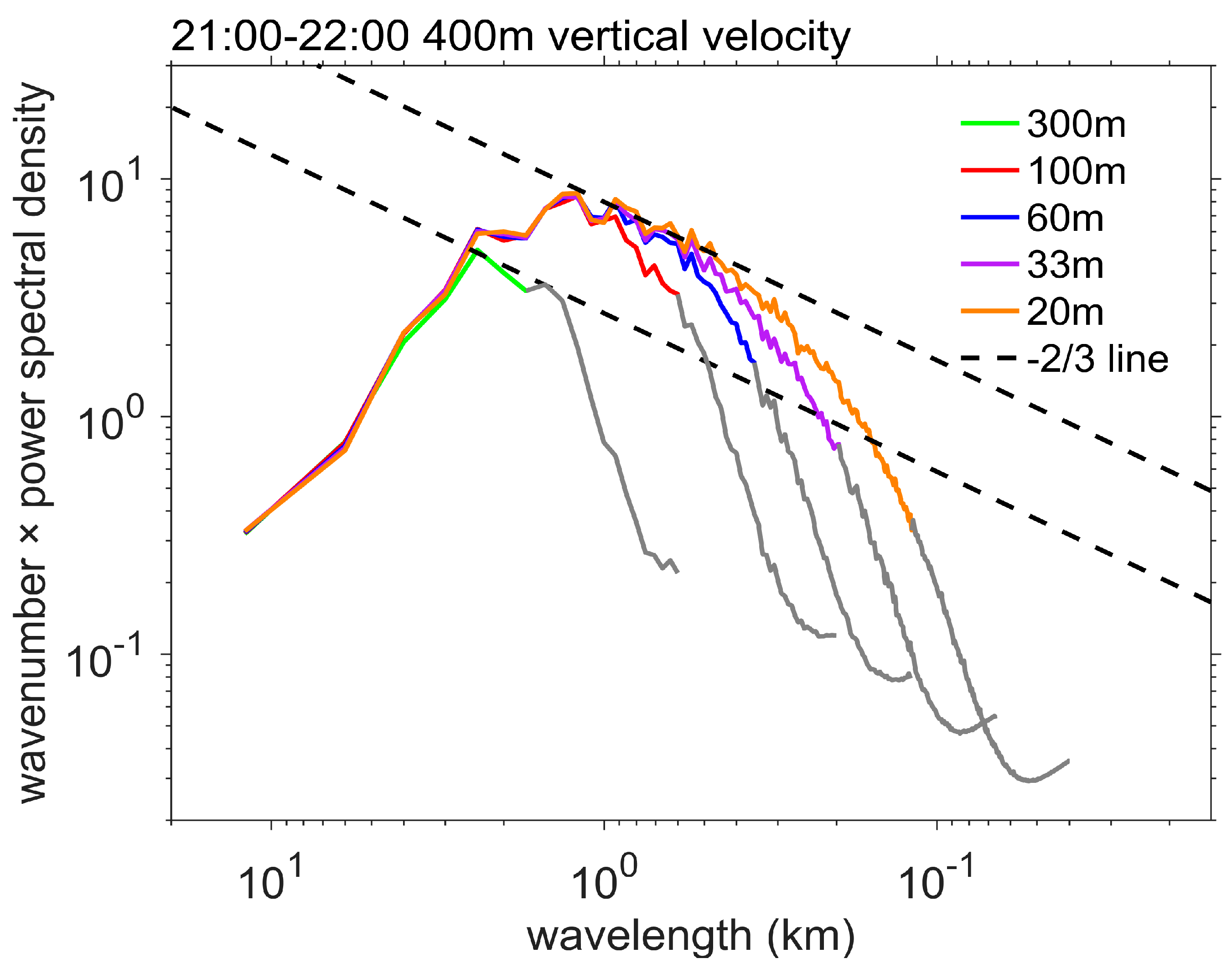
To validate the findings from Figure 7, we conducted further analyses on the simulated turbulent energy spectra obtained from LESs with different grid resolutions. Figure 8 illustrates the turbulent energy spectra of vertical velocity at a height of 400 m for simulations with varying grid resolutions. In Figure 8, the gray lines represent the small-scale wavelengths smaller than six grid spacings, as only the portion of spectra with wavelengths greater than six grid spacings can represent robust physical solutions [59]. While all simulations exhibit an intermediate range that approximately adheres to the Kolmogorov power law of turbulence, simulation d04 fails to capture the peak energy at the scale of about 1 km, which is seen in simulations from d05_1 to d06_2. Additionally, the resolved turbulent energy peak in d04 shifts towards larger scales. These observations indicate that the inadequate grid resolution of d04 prevents it from accurately resolving hectometer-scale energy-containing eddies. This deficiency significantly impacts the performance of LESs. In contrast, the similarity in turbulent energy spectra produced by simulations d05_1 to d06_2 suggests a convergence of LESs in terms of turbulence energetics. This finding reinforces the notion that a grid resolution of 100 m or finer is acceptable for LES applications in TC simulations.
4. Summary and Discussion
The objectives of this study are to investigate the sensitivity of TC simulations to the grid resolution of LESs and examine whether LESs of a TC will converge when grid resolutions are sufficiently high. To do so, LES experiments with different grid resolutions of 300 m, 100 m, 60 m, 33 m, and 20 m are performed to simulate the turbulent flow in a high wind area of Typhoon Chanthu (2021) near the radius of maximum wind speed. The main results from the performed LESs are summarized as follows.
An LES with a finer resolution produces smaller local SLPmin, larger grid-point U10max associated with the individual turbulent eddies resolved by the grids, but smaller U10ave of an area due to the cancellation of local wind maxima and minima. Second, despite the distinctive turbulent eddies resolved in the different resolution simulations, the global spatial distribution of U10 is similar for all the simulations, suggesting that for a limited area LES, model grid resolution may alter the local turbulence structure substantially, it does not appear to have a strong impact on the basic flow structure at the TC vortex scale. This conclusion is also supported by the changes in vertical distribution of the wind, temperature, and humidity in our simulations. The change in model grid resolution only shows a marginal impact on the median values of temperature, humidity, and winds throughout the vertical column, but produces significantly different extreme values directly associated with the resolved turbulent eddies. Third, all simulations are able to capture the turbulent roll vortices in the TC boundary layer. But the structure and intensity of the rolls vary substantially in different resolution simulations. For example, local hectometer-scale eddies with vertical velocity exceeding 10 m s−1 are only observed in the 20 m resolution simulation but not in the coarser resolution simulations. Fourth, the ratio of the resolved turbulent momentum fluxes and TKEs to the total momentum fluxes and TKEs in our simulations appear to show some convergence of LESs in terms of these two second-order turbulent moments when the grid resolution reaches 100 m or finer, suggesting that 100 m or smaller is an acceptable grid spacing for LES applications in TC simulations. This conclusion is supported by the turbulent energy spectrum analyses. Finally, it should be noted that, due to the limitation of computational resources, our simulations and analyses are performed only on a limited area covering 12 km × 12 km near the radius of maximum wind of Typhoon Chanthu (2021). While the conclusions may be extended to other areas with slower wind speeds in a TC based on the previous findings [25,60], it remains unknown whether they can hold for Giga-LESs that cover the entire TC vortex. This is important and needs to be tackled in future when sufficient computational resources are available.
Author Contributions
Conceptualization, Y.J., H.W., P.Z. and Y.L.; methodology, Y.J., P.Z. and Y.L.; software, Y.J., H.W., Y.L. and L.Y.; validation, H.W., P.Z., Y.L., L.Y., L.J. and A.W.; formal analysis, Y.J., H.W., P.Z. and Y.L.; investigation, H.W., P.Z., Y.L., L.Y., L.J. and A.W.; resources, Y.L.; data curation, Y.J. and Y.L.; writing—original draft preparation, Y.J. and Y.L.; writing—review and editing, H.W., P.Z., L.Y., L.J. and A.W.; visualization, Y.J. and Y.L.; supervision, H.W., P.Z., Y.L., L.Y.; project administration, Y.L.; funding acquisition, Y.L. All authors have read and agreed to the published version of the manuscript.
Funding
This research was funded by the National Natural Science Foundation of China, grant number 42075072.
Data Availability Statement
NCEP GDAS 0.25° resolution data used for the model runs are available at https://doi.org/10.5065/D65Q4T4Z (accessed on 27 July 2023).
Acknowledgments
The numerical calculations in this paper were completed on the supercomputing system in the Supercomputing Center of Nanjing University of Information Science & Technology.
Conflicts of Interest
The authors declare no conflict of interest.
References
- Nolan, D.S.; Zhang, J.A.; Stern, D.P. Evaluation of planetary boundary layer parameterizations in tropical cyclones by comparison of in situ observations and high-resolution simulations of Hurricane Isabel (2003). Part I: Initialization, maximum winds, and the outer-core boundary layer. Mon. Weather Rev. 2009, 137, 3651–3674. [Google Scholar] [CrossRef]
- Liu, J.; Zhang, F.; Pu, Z. Numerical simulation of the rapid intensification of Hurricane Katrina (2005): Sensitivity to boundary layer parameterization schemes. Adv. Atmos. Sci. 2017, 34, 482–496. [Google Scholar] [CrossRef]
- Tang, J.; Zhang, J.A.; Kieu, C.; Marks, F.D. Sensitivity of hurricane intensity and structure to two types of planetary boundary layer parameterization schemes in idealized HWRF simulations. Trop. Cyclone Res. Rev. 2018, 7, 201–211. [Google Scholar]
- Kepert, J.D. Choosing a boundary layer parameterization for tropical cyclone modeling. Mon. Weather Rev. 2012, 140, 1427–1445. [Google Scholar] [CrossRef] [Green Version]
- Gopalakrishnan, S.G.; Marks, F.; Zhang, J.A.; Zhang, X.; Bao, J.W.; Tallapragada, V. A study of the impacts of vertical diffusion on the structure and intensity of tropical cyclones using the high resolution HWRF system. J. Atmos. Sci. 2013, 70, 524–541. [Google Scholar] [CrossRef]
- Rai, D.; Pattnaik, S. Sensitivity of tropical cyclone intensity and structure to planetary boundary layer parameterization. Asia-Pac. J. Atmos. Sci. 2018, 54, 473–488. [Google Scholar] [CrossRef]
- Liu, J.; Zhang, H.; Zhong, R.; Han, B.; Wu, R. Impacts of wave feedbacks and planetary boundary layer parameterization schemes on air-sea coupled simulations: A case study for Typhoon Maria in 2018. Atmos. Res. 2022, 278, 106344. [Google Scholar] [CrossRef]
- Hong, S.Y.; Noh, Y.; Dudhia, J. A new vertical diffusion package with an explicit treatment of entrainment processes. Mon. Weather Rev. 2006, 134, 2318–2341. [Google Scholar] [CrossRef] [Green Version]
- Janjić, Z. Nonsingular Implementation of the Mellor-Yamada Level 2.5 Scheme in the NCEP Mesoscale Model; Office Note #437; National Centers for Environmental Prediction Office: College Park, MD, USA, 2001. [Google Scholar]
- Wyngaard, J.C. Toward numerical modeling in the “Terra Incognita”. J. Atmos. Sci. 2004, 61, 1816–1826. [Google Scholar] [CrossRef]
- Shin, H.H.; Hong, S.Y. Representation of the subgrid-scale turbulent transport in convective boundary layers at gray-zone resolutions. Mon. Weather Rev. 2015, 143, 250–271. [Google Scholar] [CrossRef]
- Ito, J.; Niino, H.; Nakanishi, M.; Moeng, C.H. An extension of the Mellor-Yamada model to the terra incognita zone for dry convective mixed layers in the free convection regime. Bound.-Lay. Meteorol. 2015, 157, 23–43. [Google Scholar] [CrossRef]
- Honnert, R.; Couvreux, F.; Masson, V.; Lancz, D. Sampling the structure of convective turbulence and implications for grey-zone parametrizations. Bound.-Lay. Meteorol. 2016, 160, 133–156. [Google Scholar] [CrossRef]
- Kitamura, Y. Improving a turbulence scheme for the terra incognita in a dry convective boundary layer. J. Meteorol. Soc. Jpn. 2016, 94, 491–506. [Google Scholar] [CrossRef] [Green Version]
- Goger, B.; Rotach, M.W.; Gohm, A.; Fuhrer, O.; Stiperski, I.; Holtslag, A.A. The impact of three-dimensional effects on the simulation of turbulence kinetic energy in a major alpine valley. Bound.-Lay. Meteorol. 2018, 168, 1–27. [Google Scholar] [CrossRef] [Green Version]
- Zhang, X.; Bao, J.W.; Chen, B.; Grell, E.D. A three-dimensional scale-adaptive turbulent kinetic energy scheme in the WRF-ARW model. Mon. Weather Rev. 2018, 146, 2023–2045. [Google Scholar] [CrossRef]
- Kurowski, M.J.; Teixeira, J. A scale-adaptive turbulent kinetic energy closure for the dry convective boundary layer. J. Atmos. Sci. 2018, 75, 675–690. [Google Scholar] [CrossRef]
- Efstathiou, G.A.; Plant, R.S. A dynamic extension of the pragmatic blending scheme for scale-dependent sub-grid mixing. Q. J. Roy. Meteor. Soc. 2019, 145, 884–892. [Google Scholar] [CrossRef] [Green Version]
- Nakanishi, M.; Niino, H. An improved Mellor–Yamada level-3 model: Its numerical stability and application to a regional prediction of advection fog. Bound.-Lay. Meteorol. 2006, 119, 397–407. [Google Scholar] [CrossRef]
- Deardorff, J.W. A numerical study of three-dimensional turbulent channel flow at large Reynolds numbers. J. Fluid Mech. 1970, 41, 453–480. [Google Scholar] [CrossRef]
- Nakanishi, M.; Niino, H. Large-eddy simulation of roll vortices in a hurricane boundary layer. J. Atmos. Sci. 2012, 69, 3558–3575. [Google Scholar] [CrossRef]
- Xiao, S.; Peng, C.; Yang, D. Large-eddy simulation of bubble plume in stratified crossflow. Phys. Rev. Fluids 2021, 6, 044613. [Google Scholar] [CrossRef]
- Li, Y.; Tang, J. Atmospheric boundary layer processes, characteristics and parameterization. Atmosphere 2023, 14, 691. [Google Scholar] [CrossRef]
- Sullivan, P.P.; Patton, E.G. The effect of mesh resolution on convective boundary layer statistics and structures generated by large-eddy simulation. J. Atmos. Sci. 2011, 68, 2395–2415. [Google Scholar] [CrossRef] [Green Version]
- Salesky, S.T.; Chamecki, M.; Bou-Zeid, E. On the nature of the transition between roll and cellular organization in the convective boundary layer. Bound.-Lay. Meteorol. 2017, 163, 41–68. [Google Scholar] [CrossRef]
- Zhou, B.; Simon, J.S.; Chow, F.K. The convective boundary layer in the terra incognita. J. Atmos. Sci. 2014, 71, 2545–2563. [Google Scholar] [CrossRef]
- Liu, M.; Zhou, B. Variations of subgrid-scale turbulent fluxes in the dry convective boundary layer at gray zone resolutions. J. Atmos. Sci. 2022, 79, 3245–3261. [Google Scholar] [CrossRef]
- Duan, Y.; Wan, Q.; Huang, J.; Zhao, K.; Yu, H.; Wang, Y.; Zhao, D.; Feng, J.; Tang, J.; Chen, P.; et al. Landfalling tropical cyclone research project (LTCRP) in China. B. Am. Meteorol. Soc. 2019, 100, ES447–ES472. [Google Scholar] [CrossRef]
- Kuznetsova, A.M.; Dosaev, A.S.; Rusakov, N.S.; Poplavsky, E.I.; Troitskaya, Y.I. Methods of the polar low monitoring and modeling. In Proceedings of the 2021 IEEE International Geoscience and Remote Sensing Symposium IGARSS, Brussels, Belgium, 11–16 July 2021; pp. 7260–7262. [Google Scholar]
- Saini, I.; Chandramouli, P.; Samaddar, A.; Ghosh, S. Quantifying tropical cyclone cloud cover using Envisat retrievals—An example of a recent severe tropical cyclone, ‘Thane’. Int. J. Remote Sens. 2013, 34, 4933–4950. [Google Scholar] [CrossRef]
- Chen, X.; Bryan, G.H.; Zhang, J.A.; Cione, J.J.; Marks, F.D. A framework for simulating the tropical cyclone boundary layer using large-eddy simulation and its use in evaluating PBL parameterizations. J. Atmos. Sci. 2021, 78, 3559–3574. [Google Scholar] [CrossRef]
- Zhu, P. A multiple scale modeling system for coastal hurricane wind damage mitigation. Nat. Hazards 2008, 47, 577–591. [Google Scholar] [CrossRef]
- Rotunno, R.; Chen, Y.; Wang, W.; Davis, C.; Dudhia, J.; Holland, G.J. Large-eddy simulation of an idealized tropical cyclone. B. Am. Meteorol. Soc. 2009, 90, 1783–1788. [Google Scholar] [CrossRef]
- Green, B.W.; Zhang, F. Numerical simulations of Hurricane Katrina (2005) in the turbulent gray zone. J. Adv. Model. Earth Syst. 2015, 7, 142–161. [Google Scholar] [CrossRef] [Green Version]
- Wu, L.; Liu, Q.; Li, Y. Prevalence of tornado-scale vortices in the tropical cyclone eyewall. Proc. Natl. Acad. Sci. USA 2018, 115, 8307–8310. [Google Scholar] [CrossRef] [PubMed] [Green Version]
- Li, Y.; Zhu, P.; Gao, Z.; Cheung, K.K. Sensitivity of large eddy simulations of tropical cyclone to sub-grid scale mixing parameterization. Atmos. Res. 2022, 265, 105922. [Google Scholar] [CrossRef]
- Li, X.; Pu, Z. Vertical eddy diffusivity parameterization based on a large-eddy simulation and its impact on prediction of hurricane landfall. Geophys. Res. Lett. 2021, 48, e2020GL090703. [Google Scholar] [CrossRef]
- Xu, H.; Wang, H.; Duan, Y. An investigation of the impact of different turbulence schemes on the tropical cyclone boundary layer at turbulent gray-zone resolution. J. Geophys. Res. Atmos. 2021, 126, e2021JD035327. [Google Scholar] [CrossRef]
- Chen, X. How do planetary boundary layer schemes perform in hurricane conditions: A comparison with large-eddy simulations. J. Adv. Model. Earth Syst. 2022, 14, e2022MS003088. [Google Scholar] [CrossRef]
- Wang, L.Y.; Tan, Z.M. Deep learning parameterization of the tropical cyclone boundary layer. J. Adv. Model. Earth Syst. 2023, 15, e2022MS003034. [Google Scholar] [CrossRef]
- Ye, G.; Zhang, X.; Yu, H. Modifications to three-dimensional turbulence parameterization for tropical cyclone simulation at convection-permitting resolution. J. Adv. Model. Earth Syst. 2023, 15, e2022MS003530. [Google Scholar] [CrossRef]
- Skamarock, W.C.; Klemp, J.B.; Dudhia, J.; Gill, D.O.; Liu, Z.; Berner, J.; Wang, W.; Powers, J.G.; Duda, M.G.; Barker, D.M. A Description of the Advanced Research WRF Model Version 4; National Center for Atmospheric Research: Boulder, CO, USA, 2019; Volume 145, p. 145. [Google Scholar]
- Lilly, D. The Representation of Small-Scale Turbulence in Numerical Simulation Experiments; Technical Report; National Center for Atmospheric Research: Boulder, CO, USA, 1966. [Google Scholar]
- Deardorff, J.W. Stratocumulus-capped mixed layers derived from a three-dimensional model. Bound.-Lay. Meteorol. 1980, 18, 495–527. [Google Scholar] [CrossRef]
- Beljaars, A.C. The parametrization of surface fluxes in large-scale models under free convection. Q. J. Roy. Meteor. Soc. 1995, 121, 255–270. [Google Scholar] [CrossRef]
- Jiménez, P.A.; Dudhia, J.; González-Rouco, J.F.; Navarro, J.; Montávez, J.P.; García-Bustamante, E. A revised scheme for the WRF surface layer formulation. Mon. Weather Rev. 2012, 140, 898–918. [Google Scholar] [CrossRef] [Green Version]
- Thompson, G.; Field, P.R.; Rasmussen, R.M.; Hall, W.D. Explicit forecasts of winter precipitation using an improved bulk microphysics scheme. Part II: Implementation of a new snow parameterization. Mon. Weather Rev. 2008, 136, 5095–5115. [Google Scholar] [CrossRef]
- Mlawer, E.J.; Taubman, S.J.; Brown, P.D.; Iacono, M.J.; Clough, S.A. Radiative transfer for inhomogeneous atmospheres: RRTM, a validated correlated-k model for the longwave. J. Geophys. Res. Atmos. 1997, 102, 16663–16682. [Google Scholar] [CrossRef] [Green Version]
- Dudhia, J. Numerical study of convection observed during the winter monsoon experiment using a mesoscale two-dimensional model. J. Atmos. Sci. 1989, 46, 3077–3107. [Google Scholar] [CrossRef]
- Dudhia, J. A Multi-layer Soil Temperature Model for MM5. In Proceedings of the Paper Presented at 6th Annual MM5 Users Workshop, Boulder, CO, USA, 27–30 June 1996. [Google Scholar]
- Kain, J.S. The Kain-Fritsch convective parameterization: An update. J. Appl. Meteorol. 2004, 43, 170–181. [Google Scholar] [CrossRef]
- National Centers for Environmental Prediction; National Weather Service; NOAA; U.S. Department of Commerce. NCEP GDAS/FNL 0.25 Degree Global Tropospheric Analyses and Forecast Grids; Research Data Archive at the National Center for Atmospheric Research, Computational and Information Systems Laboratory: Boulder, CO, USA, 2015.
- Kossin, J.P.; Schubert, W.H. Mesovortices, polygonal flow patterns, and rapid pressure falls in hurricane-like vortices. J. Atmos. Sci. 2001, 58, 2196–2209. [Google Scholar] [CrossRef]
- Deng, D.; Ritchie, E.A. High-resolution simulation of tropical cyclone Debbie (2017). Part I: The inner-core structure and evolution during offshore intensification. J. Atmos. Sci. 2023, 80, 441–456. [Google Scholar] [CrossRef]
- Liu, Q.; Wu, L.; Qin, N.; Li, Y. Storm-scale and fine-scale boundary layer structures of tropical cyclones simulated with the WRF-LES framework. J. Geophys. Res. Atmos. 2021, 126, e2021JD035511. [Google Scholar] [CrossRef]
- Li, X.; Pu, Z. Dynamic mechanisms associated with the structure and evolution of roll vortices and coherent turbulence in the hurricane boundary layer: A large eddy simulation during the landfall of Hurricane Harvey. Bound.-Lay. Meteorol. 2023, 186, 615–636. [Google Scholar] [CrossRef]
- Xu, H.; Wang, Y. Sensitivity of fine-scale structure in tropical cyclone boundary layer to model horizontal resolution at sub-kilometer grid spacing. Front. Earth Sci. 2021, 9, 707274. [Google Scholar] [CrossRef]
- Honnert, R.; Efstathiou, G.A.; Beare, R.J.; Ito, J.; Lock, A.; Neggers, R.; Plant, R.S.; Shin, H.H.; Tomassini, L.; Zhou, B. The atmospheric boundary layer and the “gray zone” of turbulence: A critical review. J. Geophys. Res. Atmos. 2020, 125, e2019JD030317. [Google Scholar] [CrossRef]
- Bryan, G.H.; Wyngaard, J.C.; Fritsch, J.M. Resolution requirements for the simulation of deep moist convection. Mon. Weather Rev. 2003, 131, 2394–2416. [Google Scholar] [CrossRef]
- Honnert, R.; Masson, V.; Couvreux, F. A diagnostic for evaluating the representation of turbulence in atmospheric models at the kilometric scale. J. Atmos. Sci. 2011, 68, 3112–3131. [Google Scholar] [CrossRef]
Figure 1.
Simulation domains of typhoon Chanthu (2021). The background shows the d04-simulated 10 m wind speed (U10, m s−1) at 22:00 UTC on 8 September 2021.
Figure 1.
Simulation domains of typhoon Chanthu (2021). The background shows the d04-simulated 10 m wind speed (U10, m s−1) at 22:00 UTC on 8 September 2021.

Figure 2.
Time series of (a) instantaneous grid minimum sea level pressure (hPa), (b) maximum 10 m horizontal wind speed (m s−1), and (c) domain-averaged 10 m horizontal wind speed (m s−1) over an area of 12 km × 12 km from LESs with different grid resolutions in the time period from 21:00 UTC to 22:00 UTC.
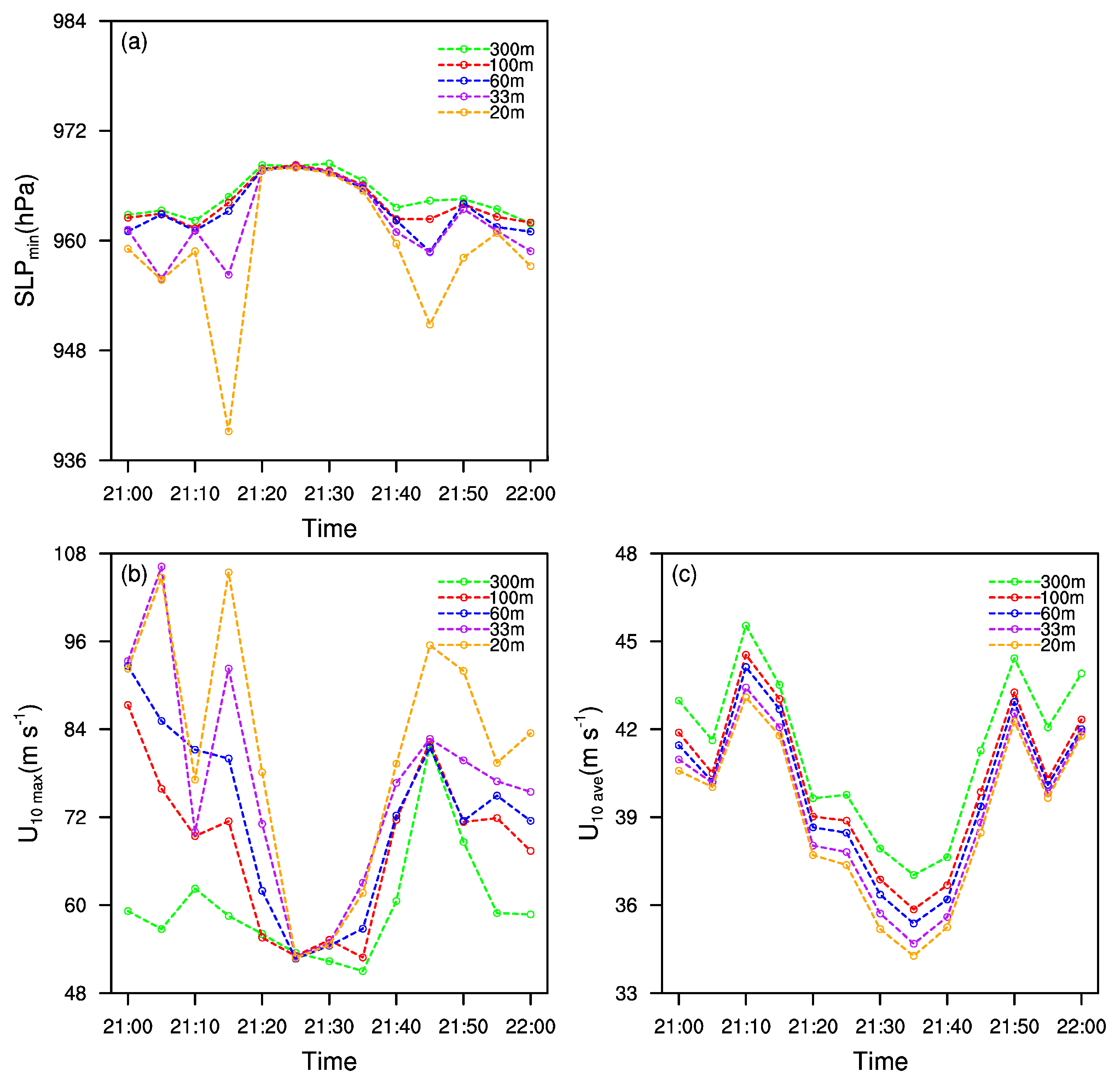
Figure 3.
(a–e) The 10 m wind speed (m s−1) averaged over the period of 21:00–22:00 UTC in the innermost 12 km × 12 km domain area for d04, d05_1, d05_2, d06_1, and d06_2, respectively. (f–i) The wind fields in d04, d05_1, d05_2, and d06_1 subtracted by those in d06_2, respectively.
Figure 3.
(a–e) The 10 m wind speed (m s−1) averaged over the period of 21:00–22:00 UTC in the innermost 12 km × 12 km domain area for d04, d05_1, d05_2, d06_1, and d06_2, respectively. (f–i) The wind fields in d04, d05_1, d05_2, and d06_1 subtracted by those in d06_2, respectively.

Figure 4.
Profiles of (a) horizontal wind speed (m s−1), (b) vertical velocity (m s−1), (c) temperature (°C), and (d) specific humidity (g kg−1) for d04 to d06_2 at 22:00 UTC in the innermost 12 km × 12 km domain. The box represents the 25th, 50th, and 75th percentiles of the data. The horizontal line spans from the minimum value to the maximum value, and the numbers next to the box represent the height above the ground in kilometers. The Y-axis is the model level, and the data shown are at an interval of 10 levels.

Figure 5.
The same as Figure 3, but for the snapshot of 10 m wind speed (U10, m s−1) at 22:00 UTC. The black dashed line oriented from southwest to northeast indicates the roll circulations resolved by LESs and is used for the vertical cross-section analyses of rolls shown in Figure 6.

Figure 6.
Vertical cross-section of vertical velocity (color shades, m s−1) and vertical structure of resolved turbulent rolls along the black dashed line shown in Figure 5 (vectors, m s−1). The green solid line in (a–e) depicts the contour line of relative vorticity equal to 0.1 s−1. Note that, to highlight the vertical overturning circulations of rolls, the mean horizontal winds over the area have been removed.
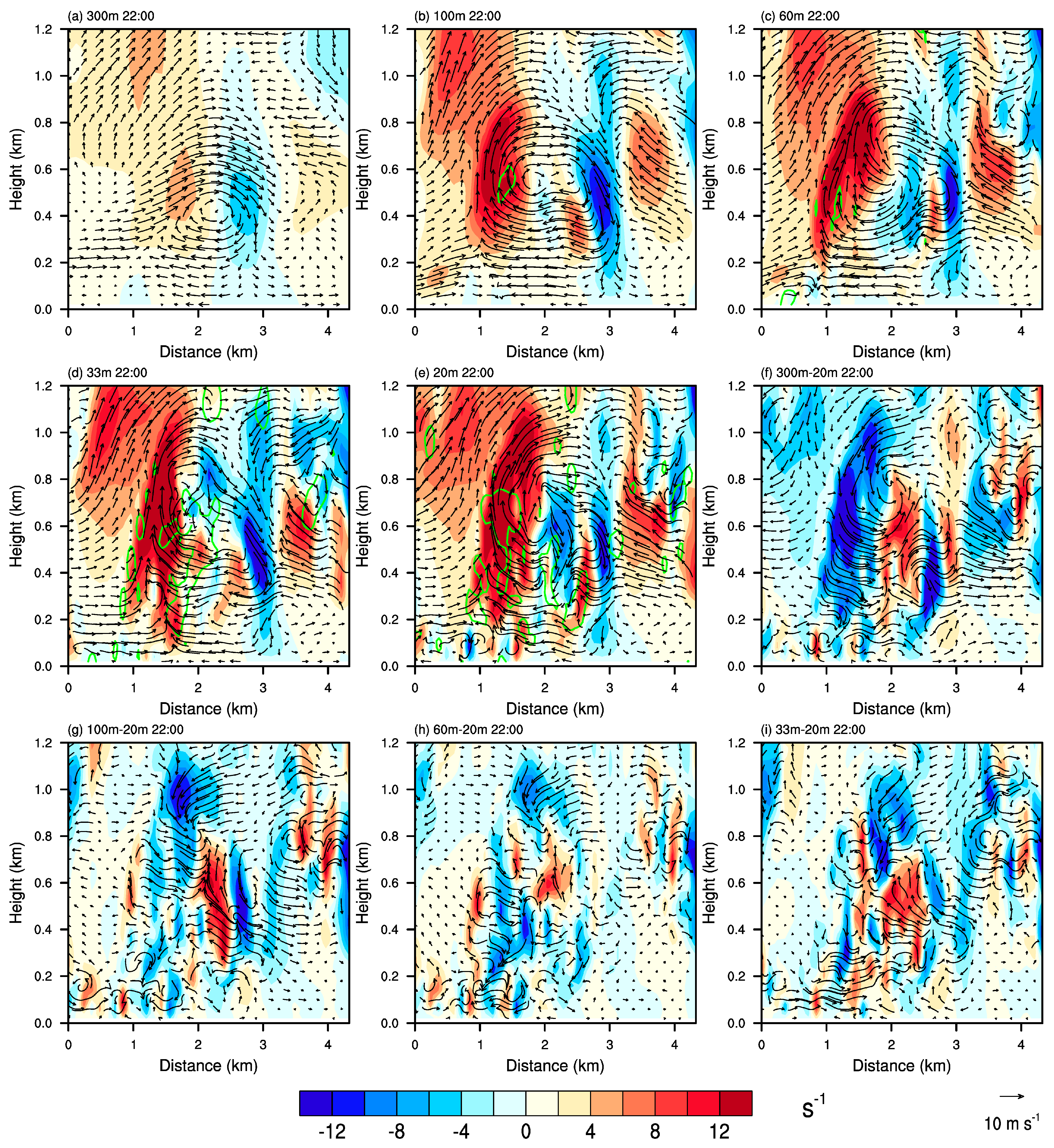
Figure 7.
Vertical profiles of turbulent momentum fluxes and TKEs from simulations with different grid resolutions averaged over the innermost domain covering an area of 12 km × 12 km and the period from 21:00 UTC to 22:00 UTC. (a) Model-resolved turbulent momentum flux (m2 s−2), (b) SGS turbulent momentum flux (m2 s−2), (c) total turbulent momentum flux (m2 s−2), (d) model-resolved TKE (m2 s−2), (e) SGS TKE (m2 s−2), and (f) total TKE (m2 s−2).
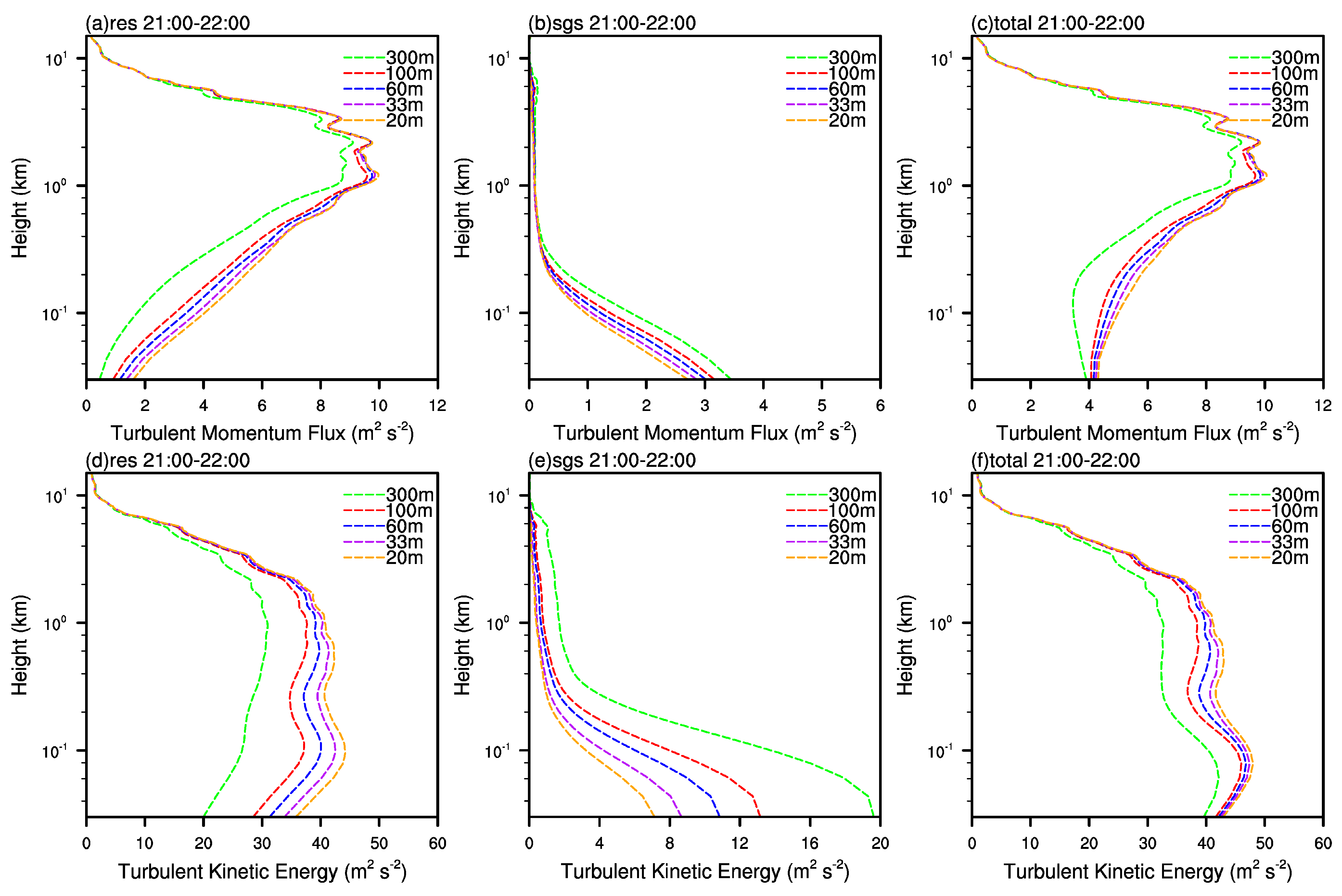
Figure 8.
Turbulent energy spectra of vertical velocity at 400 m altitude from the simulations with different grid resolutions in the innermost domain covering an area of 12 km × 12 km averaged over the period from 21:00 UTC to 22:00 UTC.
Figure 8.
Turbulent energy spectra of vertical velocity at 400 m altitude from the simulations with different grid resolutions in the innermost domain covering an area of 12 km × 12 km averaged over the period from 21:00 UTC to 22:00 UTC.

Table 1.
The settings of the domains.
| Domain Name | d01 | d02 | d03 | d04 | d05_1 | d05_2 | d06_1 | d06_2 |
|---|---|---|---|---|---|---|---|---|
| Parent domain | / | d01 | d02 | d03 | d04 | d04 | d05_1 | d05_2 |
| Horizontal resolution | 8100 m | 2700 m | 900 m | 300 m | 100 m | 60 m | 33 m | 20 m |
| Horizontal grid points | 181 × 181 | 181 × 181 | 181 × 181 | 181 × 181 | 181 × 181 | 301 × 301 | 361 × 361 | 601 × 601 |
| Timestep | 30 s | 10 s | 10/3 s | 10/9 s | 10/27 s | 2/9 s | 10/81 s | 2/27 s |
| Start time | 08_12:00 | 08_12:00 | 08_12:00 | 08_18:00 | 08_19:00 | 08_19:00 | 08_20:00 | 08_20:00 |
| End time | 08_22:00 | 08_22:00 | 08_22:00 | 08_22:00 | 08_22:00 | 08_22:00 | 08_22:00 | 08_22:00 |
| Output interval | 30 min | 30 min | 30 min | 5 min | 5 min | 5 min | 5 min | 5 min |
Disclaimer/Publisher’s Note: The statements, opinions and data contained in all publications are solely those of the individual author(s) and contributor(s) and not of MDPI and/or the editor(s). MDPI and/or the editor(s) disclaim responsibility for any injury to people or property resulting from any ideas, methods, instructions or products referred to in the content. |
© 2023 by the authors. Licensee MDPI, Basel, Switzerland. This article is an open access article distributed under the terms and conditions of the Creative Commons Attribution (CC BY) license (https://creativecommons.org/licenses/by/4.0/).
Share and Cite
MDPI and ACS Style
Jing, Y.; Wang, H.; Zhu, P.; Li, Y.; Ye, L.; Jiang, L.; Wang, A. The Sensitivity of Large Eddy Simulations to Grid Resolution in Tropical Cyclone High Wind Area Applications. Remote Sens. 2023, 15, 3785. https://doi.org/10.3390/rs15153785
AMA Style
Jing Y, Wang H, Zhu P, Li Y, Ye L, Jiang L, Wang A. The Sensitivity of Large Eddy Simulations to Grid Resolution in Tropical Cyclone High Wind Area Applications. Remote Sensing. 2023; 15(15):3785. https://doi.org/10.3390/rs15153785
Chicago/Turabian StyleJing, Yi, Hong Wang, Ping Zhu, Yubin Li, Lei Ye, Lifeng Jiang, and Anting Wang. 2023. "The Sensitivity of Large Eddy Simulations to Grid Resolution in Tropical Cyclone High Wind Area Applications" Remote Sensing 15, no. 15: 3785. https://doi.org/10.3390/rs15153785
Note that from the first issue of 2016, this journal uses article numbers instead of page numbers. See further details here.