

Asymmetric Drifter Trajectories in an Anticyclonic Mesoscale Eddy

1
Shenzhen Key Laboratory of Marine IntelliSense and Computation, Shenzhen International Graduate School, Tsinghua University, Shenzhen 518055, China
2
State Key Laboratory of Marine and Environmental Science, College of Ocean and Earth Sciences, Xiamen University, Xiamen 361102, China
3
Southern Marine Science and Engineering Guangdong Laboratory (Zhuhai), Zhuhai 519000, China
4
Shenzhen Institute of Information Technology, Shenzhen 518172, China
*
Author to whom correspondence should be addressed.
Remote Sens. 2023, 15(15), 3806; https://doi.org/10.3390/rs15153806
Submission received: 19 June 2023
/
Revised: 23 July 2023
/
Accepted: 28 July 2023
/
Published: 31 July 2023
(This article belongs to the Special Issue Remote Sensing of Ocean Surface Currents: Measurement, Validation and Applications)
Abstract
:The influences of sea surface wind on the oceanic mesoscale eddy are complex. By integrating our self-developed surface drifters with satellite observations, we examined the influence of sea surface wind on the distribution of water masses and biomass within the interior of an anticyclonic eddy. Ten drifters were deployed in the northern South China Sea in the spring of 2021. Eventually, six were trapped in an anticyclonic mesoscale eddy for an extended period. Interestingly, the drifters’ trajectories were not symmetric around the eddy center, displaying a significant offset of the distance from the wind turns to the southerly wind. Particle tracking experiments demonstrated that this departure could mainly be attributed to wind-driven ageostrophic currents. This is due to the strength of wind-driven ageostrophic currents being more comparable to geostrophic currents when accompanied by a deflection between the directions of the wind-driven current and the eddy’s translation. The drifters’ derived data indicated that sub-mesoscale ageostrophic currents within the eddy contributed to this asymmetric trajectory, with Ekman and non-Ekman components playing a role. Furthermore, the evolution of ocean color data provided corroborating evidence of these dynamic processes, highlighting the importance of ageostrophic processes within mesoscale eddies.
1. Introduction
The South China Sea (SCS) is a semi-closed marginal sea that is connected with the western Pacific Ocean. Previous studies have shown that the variability of the dynamic processes in the SCS can mainly be related to wind forcings, such as the variation in the basin-wide surface currents and mesoscale eddy activity [1,2,3,4,5]. Although the large-scale processes are important and dominant in the SCS, the meso-to-submesoscale processes also play a crucial role in shaping the environment, mainly driving the cycle of energy and matter in the SCS. Nevertheless, the response signals in the mesoscale eddy, which are associated with the wind forces, have barely been discussed in previous studies due to limited observational shreds of evidence.
Mesoscale eddies, as a key component of energy and mass variations in the cascade from small to large scale, are ubiquitous in the SCS [1,6]. The typical horizontal and time scales of mesoscale eddies in the SCS are commonly considered to be around 100 km and two weeks, respectively, referring primarily to the Eulerian time scale, e.g., [1,2,6]. Mesoscale eddies are characterized by a regional sea level anomaly (SLA) [7] and also significant temperature, salinity, and chlorophyll anomalies [8,9,10]. From a more general point of view, due to the dynamical analogs to weather events in the atmosphere, mesoscale eddies in the ocean can be regarded as a spate of oceanic “weather” events [9,11]. It is easily comprehended that mesoscale eddies play a crucial role in shaping the regional climate and ocean environment in the SCS, e.g., [1,6,11,12,13].
In the SCS, the influence of wind forcing on the large-scale variation in oceanic circulations has been well documented [4,5,6,14,15]. However, the responses of a mesoscale eddy to wind forces are still an open question, especially for individual mesoscale eddy events. Previous studies are mainly limited by sparse in situ observations and the chaotic character of mesoscale eddies; therefore, the submesoscale ageostrophic motion signals associated with wind forces have rarely been captured and examined in the SCS [16,17]. If we disregard regional differences, previous studies [18,19,20,21,22] have mainly described the impacts of wind forcing on the mesoscale eddy activity and its related physical process based on the Eulerian approach and the perspective of statistical averaging. Moreover, all these studies employed the fundamental geostrophic or quasi-geostrophic (QG) approximation that the current field in mesoscale eddies satisfies the geostrophic balance [1,11,18,19]. Therefore, the wind-related ageostrophic dynamic process in mesoscale eddies is rarely discussed.
At present, we can identify mesoscale eddies directly from SLA maps [1,2,6,23]. However, these altimetric maps make it hard to resolve sub-mesoscale fluctuations. To our knowledge, the sub-mesoscale ageostrophic motion in oceanic mesoscale eddies is described as turbulence relative to mesoscale motions [24]. These physical processes can be regarded as fluctuations on smaller scales [24] and with a distinctly non-geostrophic character [25]. Due to the mesoscale eddy’s substantial horizontal displacement, sub-mesoscale ageostrophic motions within the mesoscale eddy are hard to observe merely through the Eulerian method. Nevertheless, by combining the Lagrangian and Eulerian observation data obtained from satellite altimetry and surface drifters, we have an opportunity to reveal the response characters of the mesoscale eddy from a clearer perspective [17,26].
In this study, we first screened the trajectories from six self-developed drifters deployed in the northern SCS between 28 March and 15 April 2021, which were captured by an anticyclonic eddy (AE). It was discovered that the looping drifter trajectories relative to the eddy center had an observable offset at a distance from which the dynamic mechanisms can be discussed.
2. Data and Methods
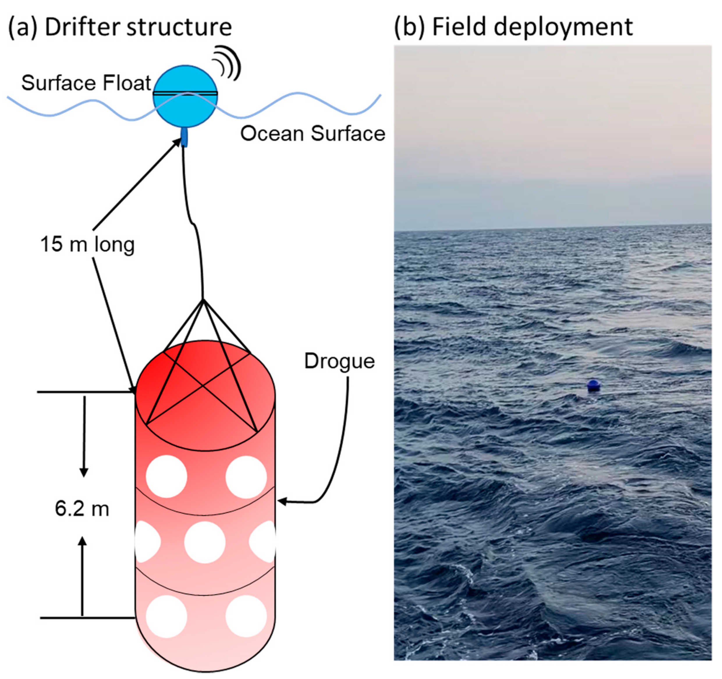
Datasets used in this study include the surface drifter’s observational data, satellite altimetric data, and reanalysis data. Lagrangian drifter observation data were obtained from 6 self-developed surface drifters. Our self-developed drifter [27,28] comprised a surface spherical float, a rope, and a holey sock drogue, as Figure 1a shows. The surface float, with a diameter of 30 cm, was tethered to a 6 m long subsurface drogue (diameter was 90 cm) by a 15 m long rope (Figure 1a). This configuration is similar to the modern satellite-tracked drifters supported and developed by the National Oceanic and Atmospheric Administration’s (NOAA’s) Atlantic Oceanographic and Meteorological Laboratory (AOML) Global Drifter Program (GDP). The drag area ratio [29] for this drifter was approximately 43, representing the ratio of the drag area for the drogue (calculated as the product of the drag coefficient and cross-sectional area) to the drag area of all other components. The drifters in this study resembled those in the previous study [29] and already showed a solid water-following capability in the field observation [27,28]. If we assumed that the surface drifts were deployed in a motionless deep-water environment, the estimated depth of the drogue’s center would be approximately 18 m. Considering the influence of oceanic currents during actual deployment, the drogue would undergo vertical inclination. If we assumed an inclination angle range of 0° to 30°, the depth at which the center of the drogue fell within the scope would be 15 m to 18 m. The drifter then uploaded the location information every 30 min. Compared to the GDP drifters, our drifters had a better temporal resolution and provided more detailed information about the variations in surface currents, which were verified to accurately reflect the actual current patterns in the SCS and the northwestern Pacific Ocean [28].
The SLA and geostrophic current anomalies data used in this study were from the Archiving, Validation, and Interpretation of Satellite Oceanographic (AVISO, available at https://www.aviso.altimetry.fr/en/ho-me.html accessed on 20 January 2023). The satellite altimetry daily data from January to July 2021 with a horizontal resolution of 1/4° × 1/4° were analyzed. We adopted the geometric vectors (GV) identification method proposed by [30] to detect mesoscale eddies in the northern SCS. When we detected a potential eddy, it was necessary to localize the search area. This localization was achieved by utilizing two parameters, a and b, defining the search area and establishing the minimum size of detectable eddies. Parameter a determined the number of points to be examined relative to a selected center point, while parameter b specified the horizontal size of the area employed to calculate the local minimum velocity. To optimize the performance of the GV method, the values of these parameters must be carefully chosen based on the data resolution. Previous studies have demonstrated that linearly interpolating the velocity field to higher-resolution grids can substantially enhance the success detection rate [2,31,32]. As the altimeter data’s horizontal resolution was limited, it could only resolve eddies with a radius larger than 25 km (equivalent to a 1/4° grid). Therefore, following [2,32], we linearly interpolated the velocity field to maintain computational efficiency while achieving the desired minimum detectable eddy size to a subgrid of 1/20° × 1/20°. This interpolation allowed for a reduction in the minimum detectable radius to 25 km, and the parameter values employed in this study (a = 5 and b = 4) were adopted from previous studies [2,32]. It can be noted that we excluded results with radii smaller than 25 km during the identification process to avoid the potential over-detection introduced by interpolation.
The atmosphere reanalysis datasets were used in this study to conduct wind slip calibration for our drifters’ positional data and estimate the ageostrophic component of the flow. The reanalysis dataset period was from 1 January to 31 December 2021. The ERA5 of the European Centre for Medium-Range Weather Forecasts (ECMWF) provided the hourly sea surface wind with a resolution of 1/4° × 1/4° [33]. In order to conduct a cross-validation analysis with ERA5, the six hourly sea surface wind datasets from Remote Sensing Systems (RSS) were also used in this study [34]. The RSS dataset with a 1/4° × 1/4° resolution was the same as the ERA5 datasets. The reason for selecting RSS wind field data for validation was primarily due to the fact that RSS provides sea surface wind data derived from state-of-the-art remote sensing instruments such as scatterometers and microwave radiometers. These instruments ensure precise measurements of the sea surface wind field. Moreover, RSS can undertake calibration and validation based on in situ data to further enhance the accuracy of their sea surface wind measurements [34]. Consequently, the exceptionally high spatiotemporal resolution and accuracy of RSS data made it highly suitable for comparative validation in this study.
To examine the influence of the sub-mesoscale ageostrophic process on the phytoplankton abundance in the mesoscale eddy interior, the key indicator in terms of the daily mean of the mass concentration from chlorophyll-a (Chl-a) data was used in this study. The Chl-a data provided by the European Copernicus Marine Environment Monitoring Service (CMEMS), with a high horizontal resolution of 4 km × 4 km, helped us resolve the sub-mesoscale structure in the eddy interior.
3. Results
3.1. Asymmetric Trajectories of Drifters
During the winter of 2020, the intrusion intensity of the Kuroshio into the SCS was extreme, as demonstrated by the AVISO satellite altimetry and our self-developed surface drifters [27]. Under the influence of Kuroshio intrusion, a strong anticyclonic eddy (AE) was generated to the west of the Luzon Strait (Figure 2a). The daily snapshot of the SLA maps displayed that this AE persisted from the beginning of December 2020 to the end of June 2021, which is a typical long-lived mesoscale anticyclonic eddy. In order to identify and track this AE, we first employed satellite altimetry data provided by AVISO to identify and statistically analyze mesoscale eddies in the northern SCS from December 2020 to June 2021 based on the GV method. This analysis provided the essential physical characteristics of the AE, such as its center point locations, radii, and amplitudes. Subsequently, we applied an eddy tracking method [35] to trace the identified mesoscale eddies, generating approximately 150 mesoscale eddy trajectories within the northern SCS region. Finally, a matching analysis was performed to compare the observations from drifters with the eddy tracking results; this allowed us to filter and select the trajectory of the AE effectively.
If we review the existing observations, we can find that the surface drifter was one of the best choices for examining the near-surface currents of the eddy [36,37,38]. Luckily and coincidentally, during the field research period in late March 2021, our research vessel happened to be sailing nearby the eddy and deployed ten surface drifters (Figure 1b). According to the criterion suggested by [39], we can consider that the drifter was captured by a mesoscale eddy only when the drifter’s trajectory presents a “looper” structure, which means that the particle’s rotation must undergo at least two consecutive loops in the same direction. Eventually, when we examined observational data, six drifters were found to be dragged into the eddy (Figure 2 and Table 1). These six drifters moved clockwise around the eddy’s center, with a period of approximately 7–10 days, to form a quasi-circular pattern (as evidenced by the spectrum result, which is not shown). Eventually, these six drifters traveled with the eddy to the northeast of the Xisha Islands, where the eddy dissipated and vanished. On average, the drifters were trapped in the eddy for 34 days, with two drifters (D514 and D615) staying inside the eddy for over 50 days.
In general, if we released a large number of particles (i.e., tracers) into the eddy interior, these particles would be advected by the geostrophic current and evenly dispersed, showing a symmetric distribution pattern [40,41]. This structure could be attributed both to the effect of geostrophic advection and diffusion on the microscopic particles. Therefore, in deep ocean regions where geostrophic currents are assumed to dominate the scenario, the drifter should move along closed streamlines in the eddy interior, and the influence of diffusion for macro-objects should be neglected (i.e., drifters). This means that if we projected the drifter position in a normalized circle, the relative position of the drifters in this normalized eddy shape would present a quasi-symmetric pattern around the eddy’s center.
The mentioned assumptions closely resembled the observation environments of our drifters. Firstly, the looping behavior depicted in Figure 2 is a characteristic pattern of a drifter trapped within a mesoscale eddy. If we expected the drifter’s motion to be primarily controlled by geostrophic currents, the relative position of the drifters in the normalized eddy shape should present a quasi-uniform symmetrical pattern. However, this symmetrical pattern only appeared in the early stage (before 8 May 2021) of our drifter observations before subsequently transforming into an asymmetrical structure. During the latter period (after 8 May 2021), the drifters’ trajectories were considerably asymmetric around the eddy center (Figure 2a). To elucidate this asymmetric phenomenon, we introduced a parameter termed “distance offset,” representing the distance between the eddy center determined from altimetry and the center of the looping trajectory. Additionally, we observed a noticeable offset between the center of the drifter’s loops and the eddy centers. As for the drifter D510 (Figure 2c), the geometry center of the loops was significantly biased to the southeast of the eddy centers, and the distance offset was ≈30 km. The other four drifters displayed similarly asymmetric tracks to the drifter D510. The only exception was drifter D512, which was only trapped in the early period and did not show such an asymmetric response. In order to analyze the reason for this difference, we conducted further analysis.
Commencing with the geostrophic balance equation, it was easy to imagine that under the control of geostrophic currents in the mesoscale eddy interior, the surface drifter (with negligible impact from diffusion) mainly moved along closed streamlines around the eddy center. The distance offset between the centers of the drifter loops and the eddy’s centers indicated that the QG balance inside the eddy was disturbed. Our drifters’ observation suggested that ageostrophic processes must occur inside the eddy and might be responsible for this asymmetric looping behavior. Previous studies have suggested that the most vigorous ageostrophic currents near the ocean’s surface are directly driven by the wind [36,42]. Upon analyzing the daily wind patterns over the northern SCS (Figure 3a), we discovered that the prevailing northeasterly winds associated with the winter monsoon quickly shifted to the southerly winds of the summer monsoon in just a few days from late April to early May, coinciding with the onset of the asymmetric looping behavior. This suggests that the different looping behaviors observed in the drifter trajectories could be related to the change in wind direction.
Prior to further investigating the relationship between the looping behavior of the drifters and the geostrophic currents and wind-forcing Ekman currents, we first derived Ekman currents from the ERA5 winds interpolated to our drifters. In this study, the near-surface Ekman velocity was estimated by an empirical formula [43]:
where is the seawater density, is determined by an unbiased linear regression model [43] and the estimation of errors in the ageostrophic velocity, and is the deflection angle of the near-surface Ekman current to the wind stress τ and varies with the latitude. It should be noted that the analysis conducted by [43] revealed that the near-surface Ekman deflection angle in our study area (15–25°N and 110–123°E) was around 55°.
Before May 2021, the wind-induced currents (Ekman) showed a similar transport direction to the AE’s movement direction (Figure 3c). This meant that even though the wind-driven current could push the drifter to move away from the eddy center, this induced offset of the distance aligned with the eddy’s moving direction and, thus, could hardly be observed. In May, the northeasterly wind turned southerly. Therefore, there was a significant deflection of directions between the wind-driven currents and the eddy’s movement, which could generate a departure in the drifters’ trajectory from the eddy center. Furthermore, initially in March, the amplitude of the currents in the eddy was over two times the wind-driven current (Figure 3b). The amplitude difference between the geostrophic and Ekman currents gradually decreased, which could be attributed to the eddy decay. From late April, the Ekman current became more comparable to the geostrophic current; therefore, the importance of the wind-driven component increased. These two conditions are probably important in generating the asymmetric response of drifters’ movement around the eddy.
3.2. Ocean Particle-Tracking Experiments
To analyze how the wind force affects the trajectory behavior of the drifters, we utilized the Ocean Parcels simulator: a tool designed for oceanic particle tracking [44]. Previous results have shown that while the drifters’ trapped dates and positions vary, all drifters exhibit similar looping behavior (Figure 2a). This indicates that we do not need to simulate the trajectory of each drifter repeatedly. With this information, we conducted a series of controlled particle tracking experiments based on the data of drifter D514. It is because D514 had the longest observational duration of 54 days among all drifters. Consequently, for simulating eddy trajectories, we utilized the location where Drifter 514 was captured as the starting point for 100 particle release points. Furthermore, the duration of particle simulation tracking was determined based on Drifter 514’s capture time and the time of its departure from the mesoscale eddy. These particle tracking experiments were designed to simulate the effects of the geostrophic and non-geostrophic conditions on the drifters’ trajectories.
For the geostrophic tracking (GT) experiment, the velocity field was derived from the satellite altimetry data provided by the AVISO. A total of 100 particles were released at 20.45–20.50°N and 116.05–116.10°E on 28 March, and then Ocean Parcel models were run to track the particle over the following three months. As Figure 4a shows, all the particles were trapped by the eddy and carried southwestward to the region around 16.0–17.5°N and 113.0–114.5°E. There was neither particle dispersion nor a distance offset between the trajectories’ looping structure and the eddy centers. The drifters were symmetrically distributed along the mesoscale eddy’s trajectory. The results of this controlled experiment confirmed that the geostrophic current could not force the departure between the eddy centers and the drifter loops’ centers.
In Section 3.1, we already computed the near-surface Ekman velocity using the Formula (1). Therefore, in the non-geostrophic tracking (nGT) experiment, we readily determined the velocity field by employing a linear combination of geostrophic and wind-driven Ekman velocities. Similar to the GT experiment, in the nGT experiment, 100 particles were released into the eddy at the same positions. The results show that only 12 particles (12%) were trapped in the eddy and eventually conveyed to the region around 16.0–17.5°N, 113.0–114.5°E, which was indicative of the particles’ dispersion (Figure 4b). The proportion that was trapped inside the eddy was consistent with the findings of a previous study [21] because when the wind-driven current did not align with the eddy’s moving direction, most of the particles were pushed away from the eddy. However, the proportion that was trapped lower than our study’s drifter observation was recorded at a percentage of 60% (6 out of 10). This could be associated with the drifters’ deployed position and date. Due to the limited drifter data available and the out scope of this study, we do not discuss this issue further. On the other hand, the particles’ trajectories in the nGT experiment show similar looping behavior to the drifters’ observation. The particle loops appeared significantly deflected to the southeast of the eddy center in the later part of the simulated period, which did not happen in the earlier stage when the wind was northeasterly and the eddy was more intense. This asymmetric response and its temporal variability agree well with the observations of the drifters’ trajectories, revealing that the wind-driven Ekman flow might be mainly responsible for such an asymmetric response to the drifter trajectories around the eddy center.
3.3. Ageostrophic Currents
Although Section 3.2 focuses on particle tracking control simulations and highlights the influence of the Ekman flow on the drifters’ deflection, it lacks a discussion on the impacts of non-Ekman ageostrophic flows. In this section, a composited analysis is conducted to obtain the spatial pattern of the ageostrophic current within the eddy interior. Particle tracking experiments were also conducted to examine the connection between non-Ekman ageostrophic currents and particle transport within the eddy.
Previous studies have suggested that when the geostrophic and windage velocities are removed from the drifters’ observational absolute velocity, the residual velocity is the ageostrophic velocity if instrument errors are neglected [45,46]. Combined with the satellite observation and reanalysis datasets, we decomposed the drifters’ absolute velocity into geostrophic and ageostrophic components: and . As we removed the geostrophic current and the windage velocity associated with the wind slip from , the ageostrophic velocity was derived, which included the wind-driven Ekman current and non-Ekman part of the ageostrophic currents such as inertial oscillations, stokes drift, tides, and centrifugation [42,46]. Here, the slip coefficient for the drogue drifters in the SCS was determined to be , as [47] estimated using the empirical method proposed by [48]. The drifters’ Lagrangian position was projected to a standard circle according to the eddy radius R, and then the spatial distribution of the velocity was obtained using linear interpolation. Then, the data were divided into two sub-periods based on the influence of the winter or summer monsoon, either prior to or after 8 May.
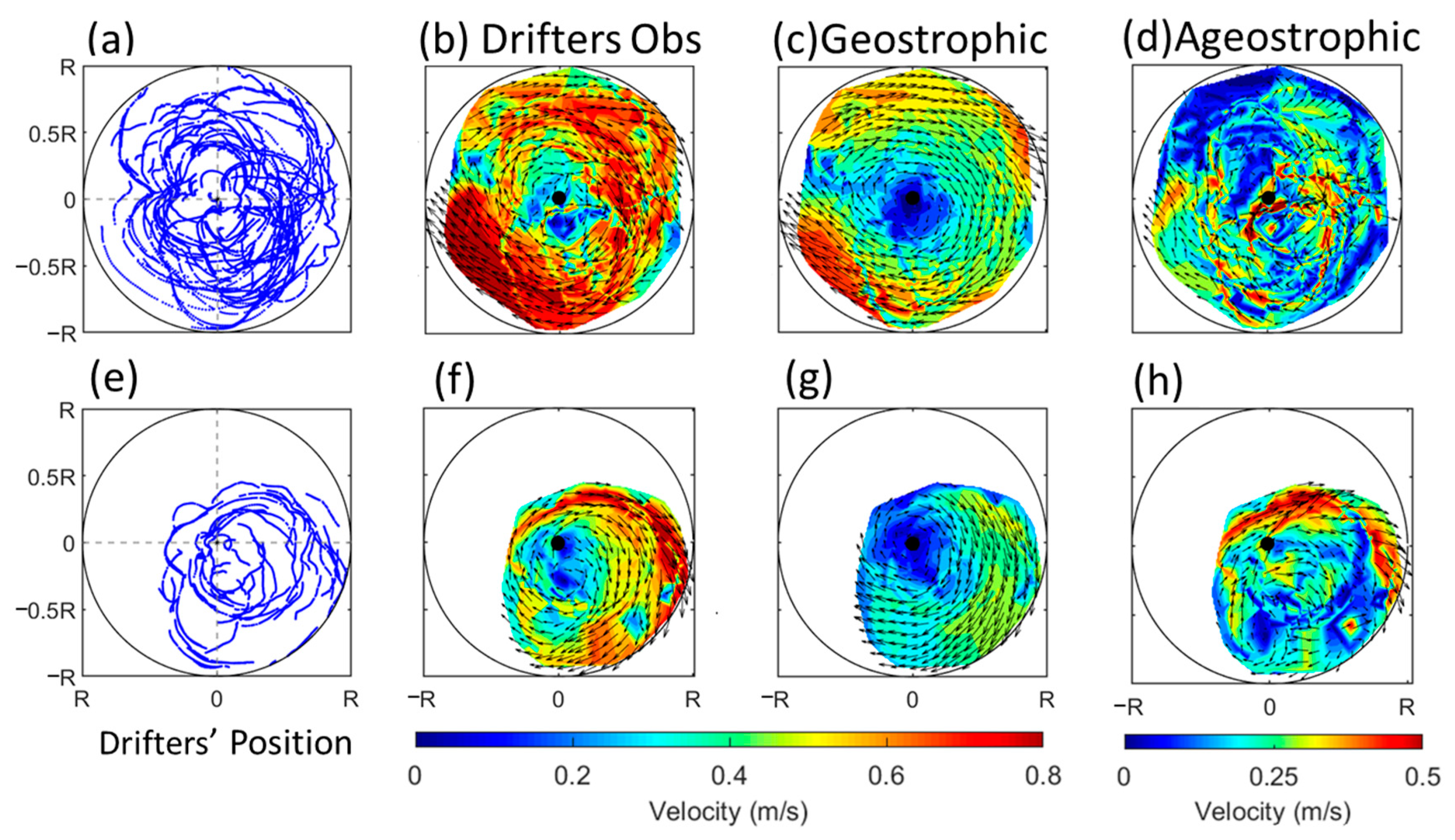
When the northeasterly wind prevailed over the SCS, the drifters’ trajectories could be symmetrically located around the eddy center (Figure 5a). Additionally, no significant offset of distance was observed between the velocity distribution derived from the drifters and the eddy center (Figure 5b). For the time that the summer monsoon dominated, the drifter’s trajectories were obviously biased from the eddy center (Figure 5e). From the drifter-derived velocity field, we could find a significant distance offset (≈30 km) from the eddy center (Figure 5f). This offset was attributed to the ageostrophic current (Figure 5h), of which the center was clearly biased from the eddy center. The ageostrophic was intensified in the eddy’s south-to-east part, where the dominant eastward or southeastward currents were driven by the wind associated with the summer monsoon. In the summer, the sub-mesoscale ageostrophic current gave rise to a nearly closed velocity filament, as shown in Figure 5h. The high velocities within these filaments not only favored the vertical displacement of nutrient-rich waters from the deep layers to the surface, thereby altering the abundance of local phytoplankton but also exerted an influence on the local phytoplankton’s abundance through horizontal transport processes [16]. Both of these influences could potentially induce alterations in the spatial distribution of phytoplankton communities within the eddy interior, which is examined in the next section.
In the control group of the particle tracking experiment (i.e., GT and nGT), we exclusively focused on assessing the impacts of Ekman currents while disregarding the effects of non-Ekman ageostrophic currents. However, by utilizing Formula (1), we could then eliminate the Ekman currents () from the drifters’ ageostrophic (, Figure 5d,h) current and obtain the non-Ekman () ageostrophic current information in the eddy interior. These new control particle-tracking experiments were conducted. Similar to the control particle tracking experiments in Section 3, we designed another group of particle-tracking experiments to evaluate the effects of the non-Ekman ageostrophic current () on the drifters’ trajectories. In the new tracking experiments, the non-Ekman ageostrophic flow field in the eddy interior was linearly combined into the daily velocity field we used in the GT and nGT experiments. It can be noted that this linear combination was divided into two subperiods, before and after 8 May 2021, as shown in Figure 5.
The geostrophic and non-Ekman ageostrophic tracking experiments (GT-nE) are shown in Figure 6a. This was the same as Figure 4a, with all the particles released at 20.45–20.50°N and 116.05–116.10°E on 28 March, which were then trapped by the eddy and carried southwestward to the region around 16.0–17.0°N and 113.0–114.0°E. One significant difference compared to the GT experiment was that in the GT-nE particle tracking experiment conducted after 8 May, a greater number of loops was observed in the trajectories of a small part of the particles, exhibiting a distinct southwestward bias. These particle movements bore similarities to the trajectories observed in the corresponding drifter data during the same period. This meant that the non-Ekman ageostrophic current could also contribute to the departure between the eddy centers and drifter loops’ centers, but not uniformly like wind-induced Ekman currents.
The new non-geostrophic tracking experiment combined the non-Ekman ageostrophic current () in the velocity field; therefore, we use nGT-nE to indicate this hereafter. The particle tracking results in the nGT-nE were almost identical to the nGT tracking experiment (c.f. Figure 6b and Figure 4b). One-hundred particles were released into the eddy, and twelve particles (12%) were trapped in the eddy and conveyed to the region around 16.0–17.5°N, 113.0–114.5°E. This meant that the influence of the non-Ekman part of the ageostrophic current on the particle distribution was mainly confined to the eddy’s interior and did not contribute to the particles’ dispersion.
After comparing the particle tracking experiment results in Figure 4 and Figure 6, we suggest that the appearance of the loop structures in the drifter trajectories, which were biased toward the southwest of the eddy center after 8 May, could be primarily attributed to the significant forcing effect exerted by large-scale wind-induced Ekman currents on the mesoscale eddy. Meanwhile, the sub-mesoscale residual ageostrophic (non-Ekman part) processes within the mesoscale eddy also contributed to this phenomenon. Based on the composite and particle tracking analysis, we concluded that the spatial asymmetry of the drifters’ looping trajectories could be regarded as the asymmetry response of the mesoscale eddy to the surface wind forcing. This is because, in addition to the direct connection between the Ekman flow and the sea surface wind field, the non-Ekman part of the ageostrophic flow observed by the surface drogue drifters also directly connected with the sea surface wind field in a large frequency band [49]. The asymmetry pattern allowed us to map the details of the submesoscale ageostrophic flow inside a mesoscale eddy and helped us understand the dynamic mechanism.
3.4. Temporal and Spatial Evolution of Chl-a within the Mesoscale Eddy
In Figure 5e, we can observe how the loop structure of the drifter predominantly leaned toward the southeastern side of the eddy. As the drogue drifter exhibited strong water-following capabilities [26], it implies that the large-scale wind forcing seemed to push a large portion of the water or substances toward the southeastern side of the eddy. Consequently, this led us to consider another question: can this phenomenon be observed from satellite observations of ocean color images? To answer this question, the daily concentration of Chl-a data was examined.
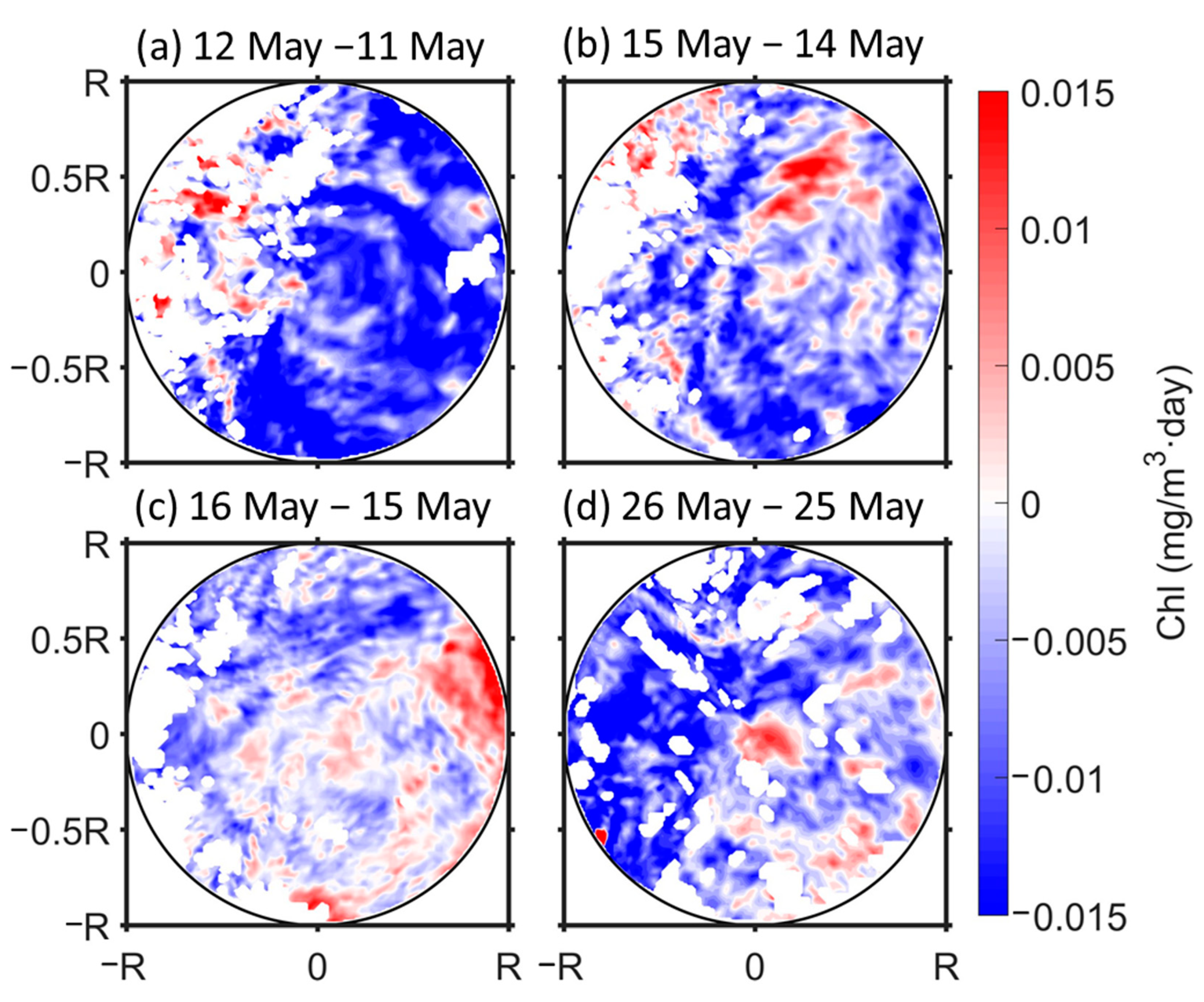
To investigate whether a similar southeastward enrichment existed in the daily change in Chl-a within the mesoscale eddy, we needed to calculate the daily trend of Chl-a. Before calculating Chl-a’s daily variation trend, seasonal variations were eliminated based on a twenty-year climatological mean from 1993 to 2022. We matched the satellite-observed Chl-a map from 1 March to 31 May with the mesoscale eddies identified in this study. In analyzing satellite observations of ocean color imagery, only the data under clear sky conditions over the eddy region were selected from those acquired for subsequent analysis. Ultimately, we obtained a seven-day dataset from the satellite observation that adequately covered the eddy region of interest, encompassing four consecutive dates. Based on this dataset, we obtained four maps representing the evolution of the Chl-a’s daily trend in the mesoscale eddy interior (Figure 7).
As displayed in Figure 7a–d, during the summer monsoon transition period (as shown in Figure 3a) in the SCS on 11/12 May 2021, there was a predominant enrichment of Chl-a to the northwest of the eddy. However, in the subsequent evolution on 14/15/16 May and 25/26 May 2021, a clear enrichment process was evident on the southeastern side of the eddy. The process of Chl-a enrichment in the southeastern part of the eddy following the onset of the summer monsoon was highly consistent with the asymmetric structure observed by the drifters. Moreover, a careful comparison between the spatial structures of the daily Chl-a trend in Figure 7d and the sub-mesoscale ageostrophic Figure 5h revealed a high degree of similarity. This denotes that the daily change in Chl-a in the eddy’s interior did not relate to the sub-mesoscale ageostrophic filament. Additionally, this southeastward bias of Chl-a enrichments could be seen as a result of the summer monsoon’s forcing, which could push the drifter or phytoplankton into the southeast of the eddy.
4. Summary and Conclusions
In spring 2021, we deployed ten surface drifters in the northern South China Sea. Six of them were trapped in a strong anticyclonic eddy for an average of 34 days. The drifters looped around the eddy and moved along with the eddy’s southwestward translation. Surprisingly, the looping trajectories displayed a significant offset of the distance from the eddy center, which mainly occurred after 8 May when the prevailing northeasterly wind associated with the winter monsoon switched to the southerly wind of the summer monsoon. Under the influence of the northeasterly wind, the Ekman current was relatively smaller than that of the eddy, and the direction of the Ekman current was close to that of the moving eddy, which probably both suppressed this offset of distance.
Therefore, the oceanic particle tracking simulator—Ocean Parcels—was used to investigate the wind effect. A total of 100 particles were deployed in the region of interest. In the experiment with only geostrophic currents, all particles were trapped by the eddy and looped around the eddy center symmetrically without a distinct distance offset. When the current was a linear combination of geostrophic and wind-driven Ekman currents, the distance offset was present after the wind turned southerly, which was similar to the drifters’ trajectories. However, only 12 particles were trapped in the eddy, indicating a much lower proportion (12%) that were trapped compared to the drifters (60%). This is because, under the influence of the monsoon, the steady wind direction could lead to an Ekman flow that tended to keep pushing the particles in the same direction to move them out of the eddy.
The drifter data were projected to a normalized eddy shape using the composite method. After removing the wind slip effect and geostrophic currents, the residual was ageostrophic. When the southerly wind prevailed, the ageostrophic current intensified in the eddy’s northern and eastern parts. This area was dominated by eastward or southeastward currents that are probably wind-driven Ekman and non-Ekman ageostrophic flows. Additionally, the ageostrophic current showed an almost closed filament, which favored the keeping and transportation of phytoplankton or drifters into the southeast part of the eddy. By analyzing satellite observations of ocean color images, we confirmed the impact of submesoscale filaments on the distribution of Chl-a within the mesoscale eddy. This is consistent with the asymmetric deflection of trajectories that were observed from drifters, indicating that the ageostrophic processes within the mesoscale eddy could be considered a response to the forcing of the surface wind field.
Previous studies have pointed out that there is a non-negligible difference between the satellite altimetry and Lagrangian drifter’s observation in the ocean near-surface velocity [42,45,50]. One new finding of this study is that surface wind stresses substantially impact mesoscale eddies through a limited case study in the SCS, which has not been reported before due to the absence of direct observational evidence. Meanwhile, due to the dynamic characteristics of eddies being similar worldwide, the findings in this study should help us further understand the wind-related process within the inner mesoscale eddy. Moreover, much is still unknown about the differential impacts of various ageostrophic on the sub-mesoscale asymmetry process in the eddy interior and how this is modulated by the surface wind. Such issues are not addressed in this study and warrant further investigation.
Author Contributions
Conceptualization, P.T., S.C. and J.H.; methodology, P.T. and S.C.; formal analysis, P.T.; drifter data collection, Z.H. and S.C.; writing—original draft preparation, P.T. and S.C.; writing—review and editing, S.C., J.H. and P.Y.; visualization, P.T. and S.C.; supervision, S.C. All authors have read and agreed to the published version of the manuscript.
Funding
This study is supported by funds from the Shenzhen Science and Technology Innovation Committee (WDZC20200819105831001), the National Natural Science Foundation of China (91958203), and the Shenzhen Key Laboratory of Marine IntelliSense and Computation (ZDSYS20200811142605016). S.C. is also supported by the Scientific Research Start-up Fund (QD2021021C).
Data Availability Statement
The sea level anomaly data provided by AVISO and can be downloaded from the websites of the Copernicus Marine Environment Monitoring Service (https://cds.climate.coper-nicus.eu/cdsapp#!/dataset/satellite-sea-level-global?tab=overview, accessed on 20 January 2023). The daily mean mass concentration of chlorophyll-a is provided by the European Copernicus Marine Environment Monitoring Service (https://marine.copernicus.eu/, accessed on 1 March 2023). The two types of sea surface wind: the reanalysis and satellite observation, were obtained from European Centre for Medium-Range Weather Forecasts (https://www.ecmwf.int/en/fore-casts/dataset/ecmwfreanalysisv5, accessed on 1 July 2022) and the Remote Sensing Systems (https://www.remss.com/me-asurements/ccmp, accessed on 12 July 2022), respectively. The drifter data can be obtained through the link (https://osf.io/pzj67/, accessed on 12 July 2022).
Acknowledgments
We thank the AVISO, European Centre for Medium-Range Weather Forecasts, and the Remote Sensing Systems for providing their datasets. Z.Y. Sun, L.Q. Yang, Z.Z. Chen, and J. Zhu are also appreciated for their drifter development.
Conflicts of Interest
The authors declare no conflict of interest.
References
- Chen, G.X.; Hou, Y.J.; Chu, X.Q. Mesoscale eddies in the South China Sea: Mean properties, spatiotemporal variability, and impact on thermohaline structure. J. Geophys. Res. Ocean. 2011, 116, C06018. [Google Scholar] [CrossRef]
- Tuo, P.F.; Yu, J.Y.; Hu, J.Y. The Changing Influences of ENSO and the Pacific Meridional Mode on Mesoscale Eddies in the South China Sea. J. Clim. 2019, 32, 685–700. [Google Scholar] [CrossRef] [Green Version]
- Wang, W.Q.; Wang, D.X.; Qi, Y.Q. Large scale characteristics of interannual variability of sea surface temperature in the South China Sea. Acta Oceanol. Sin. 2000, 22, 8216. [Google Scholar]
- Wang, D.; Wang, W.; Shi, P.; Guo, P.; Gan, Z. Establishment and adjustment of monsoon-driven circulation in the South China Sea. Sci. China Earth Sci. 2003, 46, 173–181. [Google Scholar] [CrossRef]
- Wang, C.; Wang, W.; Wang, D.; Wang, Q. Interannual variability of the South China Sea associated with El Niño. J. Geophys. Res. 2006, 111, C03023. [Google Scholar] [CrossRef]
- Wang, G.H.; Su, J.L.; Chu, P.C. Mesoscale eddies in the South China Sea observed with altimeter data. Geophys. Res. Lett. 2003, 30, 2121. [Google Scholar] [CrossRef] [Green Version]
- Chelton, D.B.; Schlax, M.G.; Samelson, R.M.; de Szoeke, R.A. Global observations of large oceanic eddies. Geophys. Res. Lett. 2007, 34, L15606. [Google Scholar] [CrossRef]
- Chelton, D.B.; Gaube, P.; Schlax, M.G.; Early, J.J.; Samelson, R.M. The influence of nonlinear mesoscale eddies on near-surface oceanic chlorophyll. Science 2011, 334, 328–332. [Google Scholar] [CrossRef] [PubMed]
- Chelton, D.B.; Schlax, M.G.; Samelson, R.M. Global observations of nonlinear mesoscale eddies. Prog. Oceanogr. 2011, 91, 167–216. [Google Scholar] [CrossRef]
- Dong, C.; McWilliams, J.C.; Liu, Y.; Chen, D. Global heat and salt transports by eddy movement. Nat. Commun. 2014, 5, 3294. [Google Scholar] [CrossRef] [Green Version]
- Saravanan, R.; Chang, P. Midlatitude mesoscale ocean-atmosphere interaction and its relevance to S2S prediction. In Sub-Seasonal to Seasonal Prediction; Elsevier: Amsterdam, The Netherlands, 2019; pp. 183–200. [Google Scholar]
- Hwang, C.; Chen, S.-A. Circulations and eddies over the South China Sea derived from TOPEX/Poseidon altimetry. J. Geophys. Res. Ocean. 2000, 105, 23943–23965. [Google Scholar] [CrossRef]
- Xiu, P.; Chai, F.; Shi, L.; Xue, H.; Chao, Y. A census of eddy activities in the South China Sea during 1993–2007. J. Geophys. Res. 2010, 115, C03012. [Google Scholar] [CrossRef] [Green Version]
- Hu, J.; Kawamura, H.; Hong, H.; Qi, Y. A review on the currents in the South China Sea: Seasonal circulation, South China Sea warm current and Kuroshio intrusion. J. Oceanogr. 2000, 56, 607–624. [Google Scholar] [CrossRef]
- Qu, T. Upper-Layer Circulation in the South China Sea. J. Phys. Oceanogr. 2000, 30, 1450–1460. [Google Scholar] [CrossRef]
- Qiu, C.; Yang, Z.; Wang, D.; Feng, M.; Su, J. The Enhancement of Submesoscale Ageostrophic Motion on the Mesoscale Eddies in the South China Sea. J. Geophys. Res. Ocean. 2022, 127, e2022JC018736. [Google Scholar] [CrossRef]
- Zhong, Y.; Bracco, A.; Tian, J.; Dong, J.; Zhao, W.; Zhang, Z. Observed and simulated submesoscale vertical pump of an anticyclonic eddy in the South China Sea. Sci. Rep. 2017, 7, srep44011. [Google Scholar] [CrossRef]
- Danioux, E.; Klein, P.; Rivière, P. Propagation of Wind Energy into the Deep Ocean through a Fully Turbulent Mesoscale Eddy Field. J. Phys. Oceanogr. 2008, 38, 2224–2241. [Google Scholar] [CrossRef]
- Eden, C.; Dietze, H. Effects of mesoscale eddy/wind interactions on biological new production and eddy kinetic energy. J. Geophys. Res. Ocean. 2009, 114, C05023. [Google Scholar] [CrossRef] [Green Version]
- Frenger, I.; Gruber, N.; Knutti, R.; Münnich, M. Imprint of Southern Ocean eddies on winds, clouds and rainfall. Nat. Geosci. 2013, 6, 608–612. [Google Scholar] [CrossRef]
- Rupolo, V. Observing turbulence regimes and Lagrangian dispersal properties in the oceans. In Lagrangian Analysis and Prediction of Coastal and Ocean Dynamics, 2nd ed.; Griffa, A., Kirwan, A.D., Eds.; Cambridge University Press: New York, NY, USA, 2007; pp. 231–274. [Google Scholar]
- Xu, C.; Zhai, X.; Shang, X.-D. Work done by atmospheric winds on mesoscale ocean eddies. Geophys. Res. Lett. 2016, 43, 12174–12180. [Google Scholar] [CrossRef] [Green Version]
- Chu, X.Q.; Xue, H.J.; Qi, Y.Q.; Chen, G.X.; Mao, Q.; Wang, D.X.; Chai, F. An exceptional anticyclonic eddy in the South China Sea in 2010. J. Geophys. Res. Ocean. 2014, 119, 881–897. [Google Scholar] [CrossRef]
- Pasquero, C.; Bracco, A.; Provenzale, A.; Weiss, J.B. Particle motion in a sea of eddies. In Lagrangian Analysis and Prediction of Coastal and Ocean Dynamics, 2nd ed.; Griffa, A., Kirwan, A.D., Eds.; Cambridge University Press: New York, NY, USA, 2007; pp. 89–118. [Google Scholar]
- McWilliams, J.C. Fluid dynamics at the margin of rotational control. Environ. Fluid Mech. 2008, 8, 441–449. [Google Scholar] [CrossRef]
- Zhang, Z.; Qiu, B.; Klein, P.; Travis, S. The influence of geostrophic strain on oceanic ageostrophic motion and surface chlorophyll. Nat. Commun. 2019, 10, 2838. [Google Scholar] [CrossRef] [PubMed] [Green Version]
- Sun, Z.; Hu, J.; Chen, Z.; Zhu, J.; Yang, L.; Chen, X.; Wu, X. A strong Kuroshio intrusion into the South China Sea and its accompanying cold-core anticyclonic eddy in winter 2020–2021. Remote Sens. 2021, 13, 2645. [Google Scholar] [CrossRef]
- Sun, Z.; Hu, J.; Lin, H.; Chen, Z.; Zhu, J.; Yang, L.; Hu, Z.; Wu, X. Lagrangian Observation of the Kuroshio Current by Surface Drifters in 2019. J. Mar. Sci. Eng. 2022, 10, 1027. [Google Scholar] [CrossRef]
- Niiler, P.P.; Sybrandy, A.S.; Bi, K.; Poulain, P.M.; Bitterman, D. Measurements of the water-following capability of holey-sock and TRISTAR drifters. Deep. Sea Res. Part I Oceanogr. Res. Pap. 1995, 42, 1951–1964. [Google Scholar] [CrossRef]
- Nencioli, F.; Dong, C.; Dickey, T.; Washburn, L.; McWilliams, J.C. A vector geometry–based eddy detection algorithm and its application to a high-resolution numerical model product and high-frequency radar surface velocities in the Southern California Bight. J. Atmos. Ocean Technol. 2010, 27, 564–579. [Google Scholar] [CrossRef]
- Lin, X.; Dong, C.; Chen, D.; Liu, Y.; Yang, J.; Zou, B.; Guan, Y. Three-dimensional properties of mesoscale eddies in the South China Sea based on eddy-resolving model output. Deep. Sea Res. Part I Oceanogr. Res. Pap. 2015, 99, 46–64. [Google Scholar] [CrossRef]
- Xia, Q.; Shen, H. Automatic detection of oceanic mesoscale eddies in the South China Sea. Chin. J. Oceanol. 2015, 33, 1334–1348. [Google Scholar] [CrossRef]
- Dee, D.P.; Uppala, S.M.; Simmons, A.J.; Berrisford, P.; Poli, P.; Kobayashi, S.; Andrae, U.; Balmaseda, M.; Balsamo, G.; Bauer, P.; et al. The ERA-Interim reanalysis: Configuration and performance of the data assimilation system. Q. J. R. Meteorol. Soc. 2011, 137, 553–597. [Google Scholar] [CrossRef]
- Mears, C.; Lee, T.; Ricciardulli, L.; Wang, X.; Wentz, F. Improving the Accuracy of the Cross-Calibrated Multi-Platform (CCMP) Ocean Vector Winds. Remote Sens. 2022, 14, 4230. [Google Scholar] [CrossRef]
- Chaigneau, A.; Gizolme, A.; Grados, C. Mesoscale eddies off Peru in altimeter records: Identification algorithms and eddy spatio-temporal patterns. Prog. Oceanogr. 2008, 79, 106–119. [Google Scholar] [CrossRef]
- Lumpkin, R.; Özgökmen, T.; Centurioni, L. Advances in the application of surface drifters. Ann. Rev. Mar. Sci. 2017, 9, 59–81. [Google Scholar] [CrossRef] [Green Version]
- Stewart, R.H. Introduction to Physical Oceanography; Department of Oceanography Texas A & M University: College Station, TX, USA, 2008. [Google Scholar]
- Thomson, R.E.; Emery, W.J. Data Analysis Methods in Physical Oceanography; Newnes: Amsterdam, The Netherlands, 2014. [Google Scholar]
- Richardson, P. A census of eddies observed in North Atlantic SOFAR float data. Prog. Oceanogr. 1993, 31, 1–50. [Google Scholar] [CrossRef]
- Martin, A.P.; Richards, K.J.; Law, C.S.; Liddicoat, M. Horizontal dispersion within an anticyclonic mesoscale eddy. Deep Sea Res. Part II Top. Stud. Oceanogr. 2001, 48, 739–755. [Google Scholar] [CrossRef]
- Morales-Márquez, V.; Hernández-Carrasco, I.; Fox-Kemper, B.; Orfila, A. Ageostrophic contribution by the wind and waves induced flow to the lateral stirring in the Mediterranean Sea. J. Geophys. Res. Ocean. 2023, 128, e2022JC019135. [Google Scholar] [CrossRef]
- Maximenko, N.; Lumpkin, R.; Centurioni, L. Ocean surface circulation. Int. Geophys. 2013, 103, 283–304. [Google Scholar]
- Ralph, E.A.; Niiler, P.P. Wind-driven currents in the tropical Pacific. J. Phys. Oceanogr. 1999, 29, 2121–2129. [Google Scholar] [CrossRef]
- Delandmeter, P.; Van Sebille, E. The Parcels v2. 0 Lagrangian framework: New field interpolation schemes. Geosci. Model Dev. 2019, 12, 3571–3584. [Google Scholar] [CrossRef] [Green Version]
- Niiler, P.P.; Maximenko, N.; Panteleev, G.; Yamagata, T.; Olson, D. Near-surface dynamical structure of the Kuroshio Extension. J. Geophys. Res. Ocean. 2003, 108, 1461. [Google Scholar] [CrossRef]
- Rio, M.H.; Mulet, S.; Picot, N. Beyond GOCE for the ocean circulation estimate: Synergetic use of altimetry, gravimetry, and in situ data provides new insight into geostrophic and Ekman currents. Geophys. Res. Lett. 2014, 41, 8918–8925. [Google Scholar] [CrossRef]
- Huang, G.; Zhan, H.; He, Q.; Wei, X.; Li, B. A Lagrangian study of the near-surface intrusion of Pacific water into the South China Sea. Acta Oceanol. Sin. 2021, 40, 15–30. [Google Scholar] [CrossRef]
- Pazan, S.E.; Niiler, P.P. Recovery of near-surface velocity from undrogued drifters. J. Atmos. Ocean Technol. 2001, 18, 476–489. [Google Scholar] [CrossRef]
- Rio, M.H.; Hernandez, F. High-frequency response of wind-driven currents measured by drifting buoys and altimetry over the world ocean. J. Geophys. Res. Ocean. 2003, 108, 1655. [Google Scholar] [CrossRef]
- Lumpkin, R. Global characteristics of coherent vortices from surface drifter trajectories. J. Geophys. Res. Ocean. 2016, 121, 1306–1321. [Google Scholar] [CrossRef] [Green Version]
Figure 1.
(a) Schematic diagram of the drifter structure. (b) Field deployment photo of the drifters.
Figure 1.
(a) Schematic diagram of the drifter structure. (b) Field deployment photo of the drifters.

Figure 2.
Topography in the northern SCS (units in m) and the looping trajectories from observations on the six drifters. (a) The water depth is shown by the shaded color, and the −200 m isobath is marked. The black line with red dots (with an interval of three days) denotes the trajectory of the eddy’s center. The other colored lines are the trajectories of six drifters trapped in the eddy. (b) Zoom in on the trajectory of drifter D512 with the starting and ending dates marked. (c) The same as (b) but for drifter D510.

Figure 3.
(a) The daily mean sea surface wind vector over the northern SCS (15−22°N, 115−121°E) from March to June 2021. (b) The time series of the mean geostrophic (solid black line) and wind-induced Ekman (solid blue line) speed inside the eddy. (c) The average degree of the moving direction for the eddy (solid red line) and Ekman (solid blue line) inside the eddy, the degree of which increased anti-clockwise from the east. Note here that to exclude the signals of high frequency (<2 days), a low-pass Lanczos filter was applied to the time series of Ekman speed and direction and the eddy’s moving direction.

Figure 4.
Particle tracking experiments. One-hundred particles were released in the northern SCS around 116.1°E and 20.5°N and tracked from 28 March to 24 May 2021. (a) The geostrophic experiment: the particle is driven by daily mean geostrophic currents. (b) The non-geostrophic experiment: all the tracking simulations configure the same as the geostrophic experiment, except the velocity field is a linear combination of the geostrophic and Ekman currents. The blue lines represent particles captured by the eddy, and the red line represents the particle’s trajectory selected with reference to the trajectory of D514. Note that the day of 8 May is marked with a pink triangle.
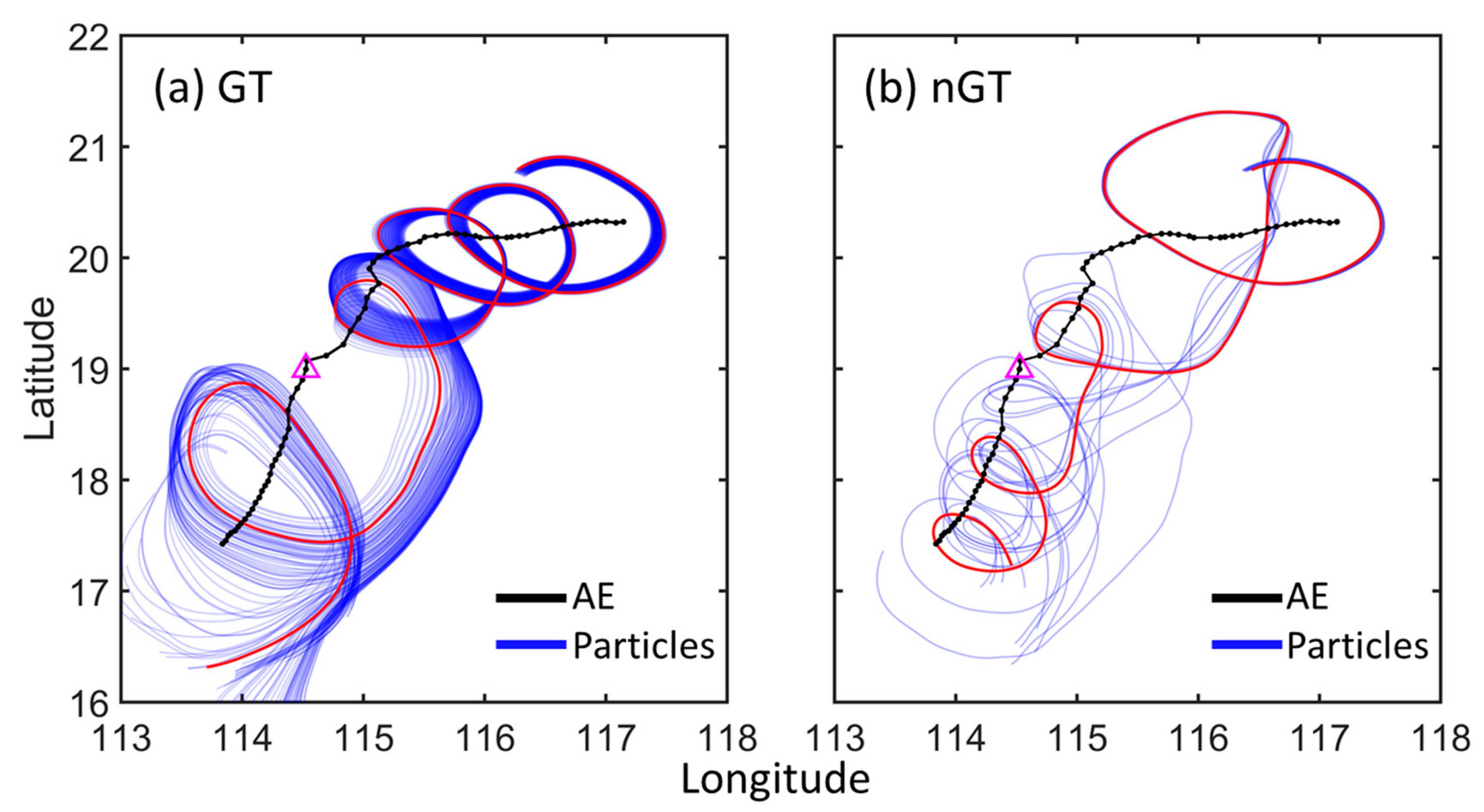
Figure 5.
The normalized drifters’ observational relative position (a,e) calibrated absolute velocity (b,f), geostrophic velocity (c,g), and ageostrophic velocity (d,h) in the anticyclonic eddy. The top panels (a–d) show the drifter observation period before 8 May 2021, and the bottom panels (e–h) show the drifter observation period after 8 May 2021. The vectors and contours represent the direction and amplitude of the velocity, respectively. The eddy center is marked with black dots.

Figure 6.
Same as Figure 4, but for the (a) geostrophic experiment and (b) non-geostrophic experiment, wherein we linearly combined the non-Ekman ageostrophic currents () derived from the drifters into the eddy interior.
Figure 6.
Same as Figure 4, but for the (a) geostrophic experiment and (b) non-geostrophic experiment, wherein we linearly combined the non-Ekman ageostrophic currents () derived from the drifters into the eddy interior.

Figure 7.
The daily trend of the Chl-a concentration in the eddy interior (Units ).

Table 1.
Identification number of drifters and trapped days at various capture positions by the anticyclonic mesoscale eddy in the northern SCS.
Table 1.
Identification number of drifters and trapped days at various capture positions by the anticyclonic mesoscale eddy in the northern SCS.
| Drifter No. | Date of Capture | Date of the End | Trapped Days | Capture Position |
| D510 | 28 April 2021 | 18 May 2021 | 20 | 114.9°E, 17.8°N |
| D512 | 31 March 2021 | 29 April 2021 | 29 | 116.1°E, 19.3°N |
| D514 | 30 March 2021 | 23 May 2021 | 54 | 116.0°E, 20.5°N |
| D515 | 15 April 2021 | 18 May 2021 | 33 | 116.1°E, 19.8°N |
| D517 | 15 April 2021 | 2 May 2021 | 17 | 116.4°E, 19.8°N |
| D615 | 29 March 2021 | 19 May 2021 | 51 | 115.8°E, 20.8°N |
Disclaimer/Publisher’s Note: The statements, opinions and data contained in all publications are solely those of the individual author(s) and contributor(s) and not of MDPI and/or the editor(s). MDPI and/or the editor(s) disclaim responsibility for any injury to people or property resulting from any ideas, methods, instructions or products referred to in the content. |
© 2023 by the authors. Licensee MDPI, Basel, Switzerland. This article is an open access article distributed under the terms and conditions of the Creative Commons Attribution (CC BY) license (https://creativecommons.org/licenses/by/4.0/).
Share and Cite
MDPI and ACS Style
Tuo, P.; Hu, Z.; Chen, S.; Hu, J.; Yu, P. Asymmetric Drifter Trajectories in an Anticyclonic Mesoscale Eddy. Remote Sens. 2023, 15, 3806. https://doi.org/10.3390/rs15153806
AMA Style
Tuo P, Hu Z, Chen S, Hu J, Yu P. Asymmetric Drifter Trajectories in an Anticyclonic Mesoscale Eddy. Remote Sensing. 2023; 15(15):3806. https://doi.org/10.3390/rs15153806
Chicago/Turabian StyleTuo, Pengfei, Zhiyuan Hu, Shengli Chen, Jianyu Hu, and Peining Yu. 2023. "Asymmetric Drifter Trajectories in an Anticyclonic Mesoscale Eddy" Remote Sensing 15, no. 15: 3806. https://doi.org/10.3390/rs15153806
Note that from the first issue of 2016, this journal uses article numbers instead of page numbers. See further details here.