

Retrieving Sub-Canopy Terrain from ICESat-2 Data Based on the RNR-DCM Filtering and Erroneous Ground Photons Correction Approach

1
The School of Civil Engineering, Central South University of Forestry and Technology, Changsha 410004, China
2
Hunan Key Laboratory of Remote Sensing Monitoring of Ecological Environment in Dongting Lake Area, Hunan Natural Resources Affairs Center, Changsha 410004, China
*
Author to whom correspondence should be addressed.
Remote Sens. 2023, 15(15), 3904; https://doi.org/10.3390/rs15153904
Submission received: 4 June 2023
/
Revised: 28 July 2023
/
Accepted: 4 August 2023
/
Published: 7 August 2023
(This article belongs to the Special Issue Remote Sensing and Smart Forestry II)
Abstract
:Currently, the new space-based laser altimetry mission, Ice, Cloud, and Land Elevation Satellite-2 (ICESat-2), is widely used to obtain terrain information. Photon cloud filtering is a crucial step toward retrieving sub-canopy terrain. However, an unsuccessful photon cloud filtering performance weakens the retrieval of sub-canopy terrain. In addition, sub-canopy terrain retrieval would not be accurate in densely forested areas due to existing sparse ground photons. This paper proposes a photon cloud filtering method and a ground photon extraction method to accurately retrieve sub-canopy terrain from ICESat-2 data. First, signal photon cloud data were derived from ICESat-2 data using the proposed photon cloud filtering method. Second, ground photons were extracted based on a specific percentile range of elevation. Third, erroneous ground photons were identified and corrected to obtain accurate sub-canopy terrain results, assuming that the terrain in the local area with accurate ground photons was continuous and therefore could be fitted appropriately through a straight line. Then, the signal photon cloud data obtained by the proposed method were compared with the reference signal photon cloud data. The results demonstrate that the overall accuracy of the signal photon identification achieved by the proposed filtering method exceeded 96.1% in the study areas. The sub-canopy terrain retrieved by the proposed sub-canopy terrain retrieval method was compared with the airborne LiDAR terrain measurements. The root-mean-squared error (RMSE) values in the two study areas were 1.28 m and 1.19 m, while the corresponding (coefficient of determination) values were 0.999 and 0.999, respectively. We also identified and corrected erroneous ground photons with an RMSE lower than 2.079 m in densely forested areas. Therefore, the results of this study can be used to improve the accuracy of sub-canopy terrain retrieval, thus pioneering the application of ICESat-2 data, such as the generation of global sub-canopy terrain products.
1. Introduction
Surveying the Earth’s surface can provide primary and useful geographic information concerning the planet evolution, terrestrial ecosystem changes, earthquake assessment, landslide dynamics, polar research, and the global climate [1,2,3,4,5]. As a digital expression of the Earth’s surface, the digital elevation model (DEM) can model, analyze, and display the topography or other surfaces [6]. However, high-precision DEMs, especially the sub-canopy terrain in forested areas, are always difficult to obtain due to the dense vegetation coverage [7,8]. Although previous studies have successfully improved the accuracy of sub-canopy terrain retrieval in small areas, it is still a challenge to obtain accurate and consecutive sub-canopy terrain in large-scale areas [9,10].
Light Detection And Ranging (LiDAR), which can measure simultaneously both vegetation structure and terrain morphology with high precision, has in recent decades been widely used to acquire sub-canopy terrain [11,12]. For example, airborne LiDAR has the advantage to retrieve terrain or sub-canopy terrain and, thus, is very helpful for detecting geo-hazards, such as landslides, in mountainous areas [13,14]. The main advantage of terrestrial and airborne LiDAR systems when performing forest inventories is fast, automatic, and millimeter-level detail documentation [15]. Nevertheless, due to high data acquisition costs, the DEM and sub-canopy terrain at large spatial scales measured by the terrestrial and airborne LiDAR systems remain largely impractical. Spaceborne LiDAR can perform inexpensive and effective topographic sampling measurements almost all over the world [16,17]. The new generation of spaceborne LiDAR, ICESat-2, is equipped with the Advanced Topographic Laser Altimeter System (ATLAS) instrument, which uses micro-pulse photon-counting technology with a high sampling rate and a small footprint [18]. Owing to the high-resolution and accurate elevation measurements, ICEsat-2 is considered a promising tool for retrieving sub-canopy terrain at a large scale [19]. However, during daytime data acquisition, a large number of noise photons are generated around the surface, greatly affecting the accuracy of sub-canopy terrain retrieval and even making the photon cloud data unavailable [19,20]. Hence, it is crucial to perform photon cloud filtering before retrieving sub-canopy terrain.
There exist many photon cloud filtering methods to derive pure signal photon cloud data from ICESat-2 data, and clustering-based methods are considered an effective category of filtering methods [21,22,23,24]. Popescu et al. applied a multilevel noise filtering approach to minimizing noise photons [23]. Wang et al. employed a Bayesian decision theory to propose a novel noise filter for signal photon data [24]. Furthermore, Zhang et al. designed a modified density-based spatial clustering of applications with noise (mDBSCAN) method to filter out noise photons and extract ground surface [22]. Based on the particle swarm optimization (PSO) algorithm, Huang et al. presented an automatic photon cloud filtering algorithm [21]. The methods mentioned above can obtain accurate signal photons in their study areas. Recently, Peng et al. established the high effectiveness of the direction centrality metric (DCM) to distinguish internal and boundary points into clusters, which might further improve the accuracy of the existing filtering methods [25]. However, the DCM uses the different directional distribution of internal and boundary points to effectively separate them, but mainly in the noise-free environment. We aim to filter photon cloud data by using the DCM-based cluster approach. To achieve a nearly noise-free environment, we use the relative neighboring relationship (RNR) filter to distinguish the majority of signal photons from noise photons at first.
The sub-canopy terrain is retrieved from precise signal photon cloud data. To date, many sub-canopy terrain retrieval methods with high accuracy have been proposed [23,26,27,28]. Gwenzi et al. proposed an algorithm that can automatically identify cutoff points, which indicates that cumulative density at the lowest elevation is equal to that at the mean terrain elevation [26]. Nie et al. separated ground reflection from canopy reflection using an iterative photon classification algorithm and then determined the ground surface [27]. Popescu et al. used an overlapping moving window method, combined with the cubic spline interpolation method, to identify ground photons from the filtered photons. He et al. also proposed an improved local outlier factor algorithm with a rotating search area (LOFR) to classify the ground photons obtained from filtered photons [28]. All of these methods can obtain dependable sub-canopy terrain in the specific study areas. However, due to the dense vegetation cover, the ground photons in densely forested areas are sparse, which might block the laser pulses from ATLAS to the ground and then lead to misclassification of erroneous ground photons that should be canopy photons [29]. Sub-canopy terrain retrieval methods do not fully consider that the ground photons are sparse and that the retrieved sub-canopy terrain might not be as accurate in densely forested areas. There is no criteria or assumption that has been proposed to solve the erroneous ground photons over densely forested areas. To achieve this goal, we propose an assumption to identify those erroneous ground photons and then correct them.
To summarize, the objective of this study is to generate reliable sub-canopy terrain in densely forested areas. To fulfill the objective, we propose a cluster-based filtering method to obtain the complete signal photons. Then the ground photons can be generated from signal photons for retrieving sub-canopy terrain. To achieve high-accuracy sub-canopy terrain generation, we identify and correct the erroneous ground photons in densely forested areas.
2. Materials
2.1. Study Area
Four study areas, namely, the Central African Republic (CA), Loudon Town (LD), BOW Town (BOW), and Harvard Forest (HARV), were used to verify the proposed method. Figure 1 displays the geographical locations of the four study areas and the distribution of the spaceborne LiDAR (ICESat-2) data and the airborne LiDAR digital terrain model (DTM) data.
The CA region in Figure 1a is located in the tropical rainforests of the Central African Republic and has an enormous vegetation cover. Both the LD region in Figure 1b and the BOW region in Figure 1c are located in New Hampshire, USA, and are covered by seasonal deciduous forests dominated by mixed forest stands. The terrain of the two sites is primarily flat, and the vegetation coverage in some local areas is high. The HARV region in Figure 1d, which is in Massachusetts, USA, displays an undulating terrain and a high vegetation cover comprising seasonal deciduous and mixed forests. Specifically, two study areas (namely, BOW and HARV) were used to assess the sub-canopy terrain results obtained by the proposed retrieving method. Therefore, these study areas offered opportunities to assess the performance of the proposed method in challenging forested areas.
2.2. ICESat-2 Data
Although ICESat was successful, the scientific community identified the limitations of spatial resolution, spatial sampling internals, and footprint size, which prevented the full utilization of the dataset for scientific purposes. In response, NASA launched the Ice, Cloud, and Ground Elevation Satellite 2 (ICESat-2), which was considered a new space-based laser altimetry approach [18]. The ICESat-2 mission is equipped with the Advanced Topographic Laser Altimeter System (ATLAS), which enables high-resolution and accurate elevation measurements [30]. It is well known that ATLAS is a state-of-the-art LiDAR system that makes use of micro-pulse photon-counting technology to operate at a precise wavelength of 532 nm [31]. With an impressive repetition rate of 10,000 laser pulses per second on each of its six beams, ATLAS can capture intricate details about the Earth’s surface [32]. To obtain surface elevation profiles, ATLAS uses three pairs of beams separated by a distance of 3.3 km across the track, with each pair consisting of a strong and a weak beam in an approximate energy ratio of 4:1 [20]. The ground footprint diameter of ATLAS is 17 m, and the distance between adjacent footprints in the along-track direction is 0.7 m [33]. The present study utilized ICESat-2/ATL03 data for testing the proposed method, which was obtained from the National Snow and Ice Data Center (NSIDC) website at https://nsidc.org/data/atl03/versions/5 (accessed on 10 January 2023). Details about the ICESat-2 data used in the study are provided in Table 1. From Table 1, it can be observed that three of the study areas are located close to each other, while the fourth one is situated far away. However, the geographical proximity of the study areas was not a primary consideration in our research. Our main focus was on ensuring the data’s verifiability and the convenience of accessing reference data. Due to the substantial size of photon point cloud data, manual visual marking is time-consuming and labor-intensive. To address this issue, we utilized data that were pre-labeled by other researchers, containing reliable labels for signal and noise photons. Therefore, we selected these four areas as our experimental regions.
2.3. Reference Signal Photon Cloud Data
We obtained ICESat-2 reference signal photon cloud data for the four study areas, and these data were visually interpreted to identify signal areas and noise areas based on the ICESat-2/ATL03 data product [34]. The reference signal photons were used to calculate the accuracy indexes of the filtering results.
2.4. Airborne LiDAR Data
Airborne LiDAR datasets were acquired using Goddard’s LiDAR, Hyperspectral and Thermal Airborne Imager (G-LiHT) and were collected from the National Ecological Observatory Network (NEON) platform [35]. The G-LiHT system can simultaneously measures vegetation structure, foliar spectra, and surface temperatures at a high spatial resolution of approximately 1 m. With advantages such as relative inexpensiveness, robustness, portability, and high resolution, the G-LiHT is an ideal tool for evaluating the benefits of data fusion when studying terrestrial ecosystems [36]. Various types of data at three levels acquired by G-LiHT are publicly available, and Figure 1c shows the DTM of BOW collected in 2014, which belongs to Level 3 and was derived from the point cloud data in Level 1 [16]. In addition, the NEON platform offers a highly precise DTM derived from airborne LiDAR, with a reported horizontal and vertical accuracy of less than 0.4 m and 0.36 m, respectively, as specified in the Algorithm Theoretical Basis Document (ATBD) of airborne LiDAR [37]. This makes the NEON platform an ideal resource for generating high-accuracy DTMs to validate the sub-canopy terrain results. Figure 1d displays the DTM of HARV collected in 2019.
3. Methodologies
3.1. Overview of the Proposed Method
As shown in Figure 2, the flowchart of the proposed method includes three primary steps: (1) Photon Cloud Filtering, (2) Sub-canopy Terrain Retrieval, and (3) Assessment.
3.2. Photon Cloud Filtering
As the performance of sub-canopy terrain retrieval is always affected by the accuracy of signal photon cloud data, it is essential to employ a series of steps to filter out noise photons before the retrieval. Two photon cloud filtering steps, namely, Grid filtering and RNR-DCM filtering, were performed to obtain accurate signal photon cloud data. The following sections describe these filtering steps in further detail.
3.2.1. Grid Filtering
As it is not influenced by auxiliary data, the Grid filtering method was employed to eliminate noise photons far away from signal photons. The fundamental assumption of the Grid filtering method is that signal photons tend to cluster around targets such as the ground and a canopy with high density, while noise photons are likely to be randomly distributed with low density [23]. Based on this assumption, we first divided the entire photon cloud into several grids with a fixed size of 18 m for the vertical axis and 40 m for the horizontal axis, and this was determined by a trial-and-error approach that yielded optimal results for all datasets. Then, the grid with the highest photon density along the vertical and horizontal directions was found and determined to be the central signal grid. Finally, one grid below and two grids above the central signal grid were defined to be the potential signal grids, while photons outside the potential signal grids were regarded as noise photons. Thus, we removed the noise photons far away from the signal photons.
3.2.2. RNR-DCM Filtering
Despite the fact that noise photons far away from signal photons were removed by the Grid filter in Section 3.2.1, there were still noise photons adjacent to the signal photons. Thus, we employed the advanced RNR-DCM filter to remove the noise photons adjacent to the signal photons. Specifically, the RNR filter can well identify noise photons adjacent to signal photons, while the DCM filter is capable of identifying sparse clusters with low density in the noise-free environment [25,38]. The detailed procedure is outlined in the following subsections.
- (1)
- RNR Filtering
First, the RNR filter was used to remove most of the noise photons adjacent to the signal photons to provide a nearly noise-free environment. The RNR filter is based on the principle that the density of the neighbors of a noise photon adjacent to the signal photon will be slightly different from the density of the neighbors of a signal photon, as the noise photon’s neighbors will include more signal photons than pure noise photons [38]. The above phenomenon is called the RNR. We quantitatively calculated the RNR value using Equation (1) for each photon to describe the difference between signal photons and noise photons adjacent to signal photons.
where is the RNR between photon i and its jth neighbor; j is the jth neighbor photon of photon i; i is the th neighbor of photon j; and K is the number of photon neighbors.
The magnitude of the RNR illustrates the density difference between neighbor photons around photon i and photon j. The larger the value of RNR is, the greater the difference in density will be. To further quantify the RNR value of each photon in comparison to its neighboring photons, the sum of the RNR values of the K-nearest neighbor photons is calculated with Equation (2).
Since the RNR values varied in the sparse and dense photon cloud regions, we divided the photon cloud with a window of a specific size. In each window, photons whose RNR value exceeded a certain percentile value were filtered out. In this study, we empirically chose that the number of neighbors should be 30, a window size of 50 m along the horizontal direction, and a percentile range of 0.95–0.97 for removing most of the noise photons adjacent to signal photons through the RNR filter, sequentially providing a nearly noise-free environment for the DCM filter.
- (2)
- DCM Filtering
After the nearly noise-free environment was constructed (Figure 3a), the DCM filter was used to separate the remaining photons into signal photon clusters and noise photons adjacent to the signal photon clusters, and thus the noise photons adjacent to signal photons were removed. The core idea of the DCM filter is that the internal points (signal photons) are surrounded by neighboring points in all directions (Figure 3c), while the boundary points (noise photons adjacent to signal photons) only include neighboring points within a particular directional range (Figure 3b). The variance of the angles formed by a photon with its neighbors (Figure 3b,c) was defined as the DCM to describe the difference in directional distribution [25]. The value of the DCM would significantly vary between signal photons and noise photons adjacent to the signal photons, which allowed us to separate them into two clusters, so as to remove the noise photons adjacent to signal photons subsequently.
To quantify the difference between internal and boundary points, the DCM of each photon should be calculated according to Equation (3):
where K is the number of photon neighbors.
When all the angles of a photon with its neighbors are equal, the DCM reaches the minimum value of 0, indicating that the neighboring points are evenly distributed in all directions. When the neighboring points are distributed in the same direction, one of the angles of the photon is 2 and the others are 0, and thus the DCM reaches the maximum value of . As illustrated in Figure 3b,c, the DCM value of the noise photon adjacent to signal photons Q is considerably larger than that of the signal photon P, a fact that enables us to distinguish and separate the P and Q. In this study, we normalized the DCM to the range of 0–1 as follows:
To account for the varying DCM values in different types of regions, we applied a window-based filtering approach to the photon cloud. Specifically, we partitioned the photon cloud with a specific size window and considered photons with DCM values greater than the given threshold as noise photons adjacent to the cluster of signal photons in each window. We then removed the noise photons adjacent to the signal photons. In this study, we set the number of neighbors to 30, the window size to 30 m in the horizontal direction, and the percentile range to 0.95–0.96 by a trial-and-error approach.
3.3. Sub-Canopy Terrain Retrieval
After applying the two steps of photon cloud filtering, we obtained the signal photons (Figure 4a) and employed a two-step method to retrieve the sub-canopy terrain. First, we used a percentile-based method to extract the ground photons, considering that ground photons showed the lowest elevation in a given region. In this process, a horizontal sliding window with a fixed size of 50 m and a sliding step size of 10 m were used to retrieve the sub-canopy terrain, considering that the terrain in our study area was undulating and the elevation of ground photons in different areas varied. Within each window, photons with elevation values ranging from 8% to 12% of all photons were selected as ground photons. For areas that overlapped in the sliding window, we selected photons with the smallest average elevation as true ground photons.
In fact, after extracting ground photons using sliding windows, erroneous ground photons still existed in densely forested areas (Figure 4b), which should be identified and corrected. Based on the assumption that the terrain in the local area with accurate ground photons was continuous and therefore could be fitted appropriately via a straight line, the erroneous ground photons could be identified and corrected. In contrast, in the local areas with erroneous ground photons, the linear fitting effect was poor, which could be identified based on the mean error and quantitatively assessed. We therefore adopted a window with a fixed number of photons to fit the local terrain via a straight line with Equation (5) (Figure 4c).
where is the along-track distance of the photons; is the elevation of the photons; and are the coefficients of the linear equation, which are derived based on the least squares method with Equation (6).
where is the elevation of photon i, and is the fitted elevation of photon i. Thus, the fitted elevation of the photons can be derived with Equation (7).
Finally, we can calculate the mean error based on real elevation and fitted elevation with Equation (8).
where n is the number of photons. The mean error of linear fitting could be smaller for areas with accurate ground photons but larger for areas with inaccurate ground photons. We empirically set the mean error threshold to identify the erroneous ground photons. When the mean error of elevation is greater than the given threshold of erroneous ground photons, the erroneous ground photons are subsequently corrected (Figure 4d).
For the identified erroneous ground photons in the study regions, we employed a percentile-based ground photon extraction window method that regards all photons of each window, with elevation in the range of 0–10%, as true ground photons, thus removing erroneous ground photons and improving the accuracy of the sub-canopy terrain.
3.4. Assessment
For the signal photon cloud data obtained by the proposed filtering method, we assessed data accuracy based on visually interpreted reference signal photon cloud data. For the ground photons obtained by the proposed retrieving method, we first employed the Hermite interpolation method to fit them into the terrain line [39]. Thereafter, we extracted each terrain photon at 20 m intervals along the horizontal direction and quantitatively compared these terrain photons with those derived from airborne LiDAR data.
3.4.1. Assessment of Filtering Results
Four indicators, namely, the Recall Rate (R), Precision (P), F-Value (F), and Overall Accuracy (OA), were used to quantitatively assess the accuracy of the signal photon cloud obtained from ICESat-2 raw data [19]. The indicators can be calculated as follows:
where represents photons correctly classified as signal photons; represents photons correctly recognized as noise photons; represents signal photons misclassified as noise photons; and represents noise photons misclassified as signal photons.
3.4.2. Assessment of Sub-Canopy Terrain Results
Three indicators—the coefficient of determination (), standard deviation (STD), and root-mean-squared error (RMSE)—were used to quantitatively assess the accuracy of the sub-canopy terrain retrieved from ICESat-2 data.
4. Results and Discussion
4.1. Photon Cloud Filtering Results
In this study, we qualitatively and quantitatively evaluated the effectiveness of photon cloud filtering results for ICESat-2 data. First, we evaluated the performance of the proposed photon cloud filtering method by qualitative analysis, which was performed by visually comparing the filtered photon cloud data with the reference signal photon cloud data in the study areas. The results of the proposed photon cloud filtering method for the four study areas are displayed in Figure 5, Figure 6, Figure 7 and Figure 8. As shown in Figure 5, Figure 6, Figure 7 and Figure 8, there is reliable consistency between the filtered signal photon cloud data and the reference signal photon cloud data. Especially in the partially enlarged regions, the filtered photon cloud data have a significantly high consistency with the reference signal photon cloud data, a fact that confirms the reliability of the proposed photon cloud filtering method. To further evaluate the effectiveness of the proposed photon cloud filtering method, we quantitatively assessed the accuracy of the filtered signal photon cloud data chiefly based on four indicators, namely, the Recall Rate (R), Precision (P), F-Value (F), and Overall Accuracy (OA), and compared the filtered signal photon cloud data with visual-interpretation-derived reference signal photon cloud data. R indicates the proportion of the number of correctly extracted signal photons to the total number of original signal photons. P is the proportion of the number of correctly extracted signal photons to the total number of extracted signal photons. F signifies the harmonic average of the recall rate and precision, which can reflect the filtering performance by the one-signal measure [22]. OA represents the overall accuracy of the proposed filtering method in the given study areas. The assessment indicators of the proposed photon cloud filtering method are summarized in Table 2. The proposed photon cloud filtering method has a reliable accuracy in each study area. For example, in the CA study area, the number of TP photons is 18,376 and the number of TN photons is 11,984. Moreover, it can be observed that the proposed photon cloud filtering method performs well on the whole, as indicated by F and OA, which respectively exceed 0.97 and 0.96 in the given study areas. The above quantitative indicators illustrate that the proposed photon cloud filtering method is reliable and ensures the effective removal of noise photons adjacent to signal photons via the RNR-DCM filter.
4.2. Results of Sub-Canopy Terrain Retrieval
4.2.1. Ground Photon Extraction
Figure 9 and Figure 10 illustrate the overall ground photon extraction performance of study areas BOW and HARV, respectively. Subplots (b) and (c) in Figure 9 and Figure 10 provide the representative examples of parts with unqualified and qualified performance of ground photon extraction, respectively. According to Figure 9 and Figure 10, the proposed ground photon extraction method demonstrates an overall good performance in both study areas. However, despite the effective extraction, some unqualified photons still remain, especially in densely forested areas. This is primarily due to the sparsity of the ground photons in these areas and because the current extraction method is based only on the elevation percentile, without considering the number of photons. Therefore, we performed an additional step to identify and correct the erroneous ground photons.
4.2.2. Identification and Correction of Erroneous Ground Photons
To evaluate the performance of the erroneous ground photon identification and correction method, we displayed the representative identification results of the unqualified areas in BOW and HARV in Figure 11a,c, respectively, whereupon the representative identification results were compared with the corrected result in both study areas, as shown in Figure 11b,d. According to the results of erroneous ground photon correction in Figure 11, the proposed identification and correction method for erroneous ground photons demonstrates reliability in accurately identifying and effectively correcting erroneous ground photons, and the proposed method is based on the assumption that the terrain in the local areas with accurate ground photons was continuous and therefore could be fitted appropriately via a straight line. On the contrary, in the local areas with erroneous ground photons, the linear fitting effect was poor, which could be identified by the mean error and quantitatively assessed. Based on the assumption, we conducted the linear fitting and calculated the mean error to identify the erroneous ground photons and subsequently correct them by removing the erroneous ground photons.
4.2.3. Sub-Canopy Terrain Results
To assess the accuracy of sub-canopy terrain retrieval, three accuracy indicators were calculated for the terrain points, and the scatterplots of these indicators with point density are displayed in Figure 12. Figure 12a,c shows the scatterplot of ground photons before correction, while Figure 12b,d shows the scatterplot of ground photons after correction. Figure 12 shows a reliable consistency between the retrieved sub-canopy terrains and the airborne LiDAR-derived DTM, with high values, namely, 0.99 and 0.99, in BOW and HARV, respectively, and low RMSE values, namely, 1.28 m and 1.19 m, respectively. Moreover, the proposed ground photon identification and correction method improved the accuracy of sub-canopy terrain retrieval, as indicated by the high , low STD, and low RMSE of the corrected ground photons, compared to uncorrected ground photons. To be precise, the RMSE decreased from 1.56 m to 1.28 m, representing an improvement of 18.0% in BOW, whereas the RMSE decreased from 1.76 m to 1.19 m, marking an improvement of 32.3% in HARV. Furthermore, the scatterplots reveal a reduction in the number of outliers after the correction, suggesting an improvement in the accuracy of the ground photons and the effectiveness of the proposed method in the identification and correction of erroneous ground photons.
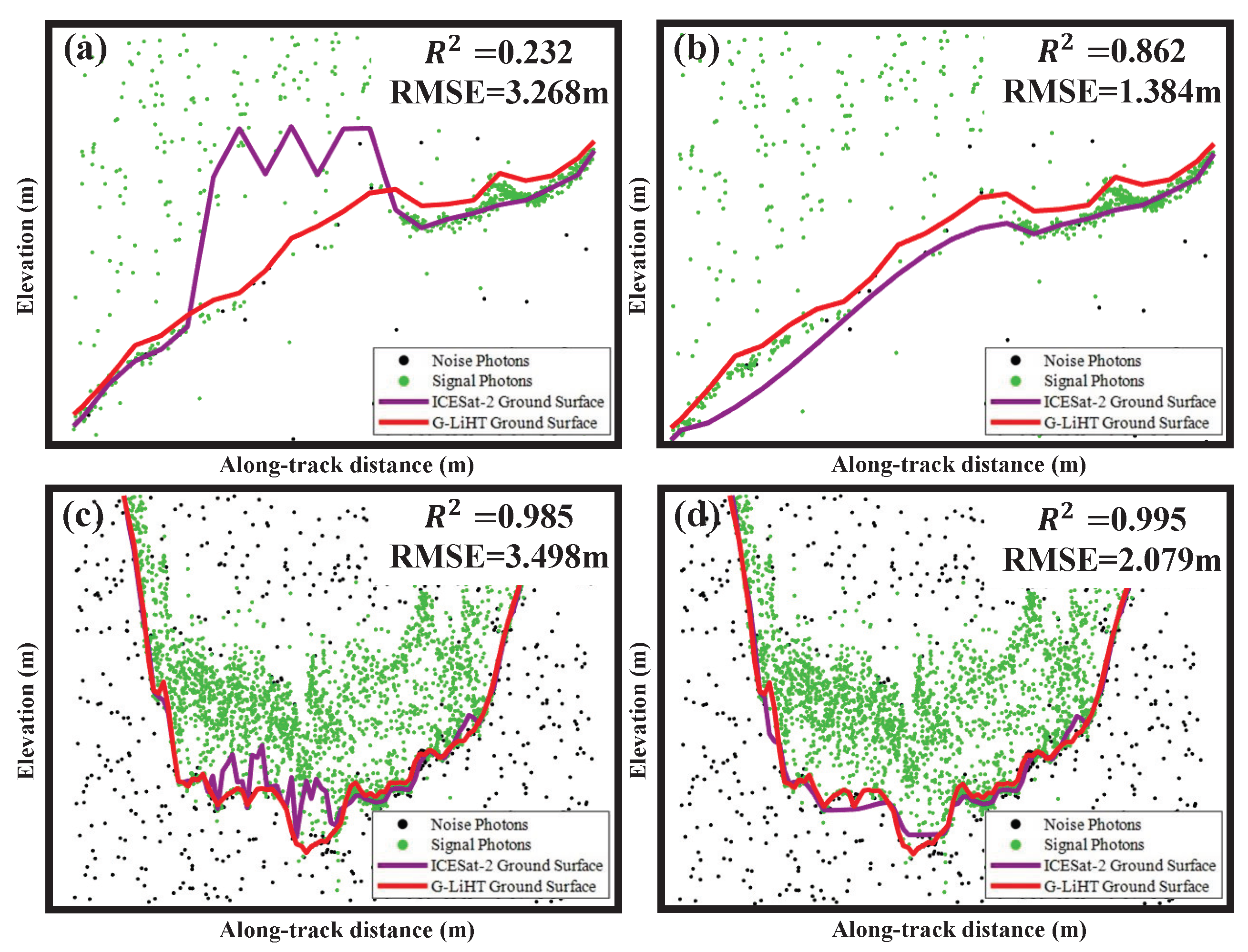
To further evaluate the effectiveness of the proposed erroneous ground photon identification and correction method, we calculated the RMSE of the erroneous terrain line interpolated by erroneous ground photons in the representative unqualified areas of BOW and HARV, which are shown in Figure 13a,c. We compared the erroneous terrain line with the corrected terrain line in both study areas, and the results are shown in Figure 13b,d. Therefore, the proposed method is reliable and can accurately identify and effectively correct the erroneous terrain line, as indicated by the high and low RMSE values of the corrected terrain line, compared to the erroneous terrain line. Specifically, in BOW, the RMSE decreased from 3.26 m to 1.38 m, indicating an improvement of 57.6%; in HARV, on the other hand, the RMSE decreased from 3.49 m to 2.07 m, signifying an improvement of 40.6%. In addition, increased from 0.232 to 0.862 in BOW, and from 0.985 to 0.995 in HARV. Moreover, Figure 13 shows that the corrected terrain lines are highly consistent with the reference terrain line, indicating the high accuracy of the terrain lines and the effectiveness of the proposed erroneous ground photon identification and correction method. Furthermore, Figure 11 demonstrates that, during the correction process, certain accurate ground photons are removed. Nonetheless, as evident from the terrain line and accuracy indicators presented in Figure 13, the precision of the retrieved terrain line remains trustworthy, even after the removal of these specific accurate ground photons. This is attributed to the primary utilization of these ground photons for fitting the terrain line. Consequently, despite the removal of some accurate ground photons under specific conditions, such as slopes, the remaining ground photons retain sufficient accuracy, enabling the retrieval of precise terrain lines.
5. Conclusions
In this study, we developed a two-stage method to filter photon cloud data and retrieve the sub-canopy terrain in forested areas. First, using the proposed photon cloud filtering method, we derived signal photon cloud data from ICESat-2 data. Second, we extracted ground photons based on a specific percentile elevation range. Third, we identified and corrected erroneous ground photons to obtain a more accurate sub-canopy terrain, based on the assumption that the terrain in the local area with accurate ground photons was continuous and therefore could be fitted appropriately through a straight line. Finally, we assessed the accuracy of the signal photon cloud data and the sub-canopy terrain based on the visual interpretation–derived signal photon cloud data and the airborne LiDAR data, respectively. To summarize, the present study leads to the following conclusions: (1) A good consistency between the filtered signal photon cloud data and the reference signal photon cloud data suggests that the proposed filtering method can remove noise photons in forested areas. (2) The results of correcting erroneous ground photons in densely forested areas indicate that the proposed method to identify and correct erroneous ground photons is suitable for sub-canopy terrain retrieval. (3) Due to the sparsity of the ground photons, the ground photons derived from densely forested areas have a large number of errors and may be misclassified as canopy photons, compared to those derived from moderately densely forested areas.
Overall, the above conclusions provide insights into the retrieval of the sub-canopy terrain in forested areas from ICESat-2 data. Because precise sub-canopy terrain retrieval is affected by the accuracy of signal photons and the density of the forest, it is necessary to further explore an effective way to obtain superior signal photons in study areas with different forest densities. Furthermore, erroneous ground photons can manifest themselves in different forms in areas with different forest densities, requiring varying levels of identification and correction intensity. Therefore, our next work will focus on the adaptive method of identifying and correcting erroneous ground photons based on the forest density.
Author Contributions
Conceptualization, Y.W. and R.Z.; methodology, Y.W. and R.Z.; software, K.Z.; validation, Y.W., R.Z. and Q.H.; formal analysis, Y.Z.; investigation, K.Z.; resources, R.Z.; data curation, K.Z.; writing—original draft preparation, Y.W.; writing—review and editing, Y.W. and Z.R.; visualization, Q.H. and Y.Z.; supervision, Q.H.; project administration, Q.H. and K.Z.; funding acquisition, R.Z. All authors have read and agreed to the published version of the manuscript.
Funding
This research was supported in part by the National Natural Science Foundation of China, grant numbers 42104016 and 41820104005, the introduction of talent research start-up fund of Central South University of Forestry and Technology, grant number 2021YJ010, and the Fundamental Research Funds for the Central Universities of Central South University, grant number 506021729. This research was also supported in part by the Open Topic Foundation of Hunan Key Laboratory of Remote Sensing Monitoring of Ecological Environment in Dongting Lake area, Grant No. DTH Key Lab.2021-012.
Data Availability Statement
The ICESat-2 data utilized in this study can be accessed freely at https://nsidc.org/data/atl03/versions/5 (accessed on 10 January 2023). Additionally, the Goddard’s LiDAR, Hyperspectral and Thermal Airborne Imager (G-LiHT) DTM data, and the National Ecological Observatory Network (NEON) DTM data, both employed in this research, are also freely available at https://glihtdata.gsfc.nasa.gov/ (accessed on 13 February 2023) and https://www.neonscience.org/ (accessed on 13 February 2023), respectively.
Acknowledgments
We would like to express our sincere appreciation to LetPub at www.letpub.com (accessed on 28 May 2023) for their invaluable linguistic assistance during the preparation of this manuscript. Additionally, we extend our heartfelt thanks to the National Aeronautics and Space Administration (NASA) for granting us access to the ICESat-2 data, and to the Goddard’s LiDAR, Hyperspectral and Thermal Airborne Imager (G-LiHT) and the National Ecological Observatory Network (NEON) for making the DTM data accessible for our research. Furthermore, we would like to extend our deep gratitude to Yi Li from Central South University for his wholehearted dedication and invaluable contributions throughout our research journey. His unwavering enthusiasm, responsiveness, and selfless provision of code have been instrumental in the success of our study. Additionally, his willingness to share knowledge without reservation has been of immense help in our endeavors. We are truly grateful for Yi Li’s outstanding support and collaborative spirit, which have significantly enriched the quality of our work.
Conflicts of Interest
The authors declare no conflict of interest.
References
- Arora, V.K. Simulating energy and carbon fluxes over winter wheat using coupled land surface and terrestrial ecosystem models. Agric. For. Meteorol. 2003, 118, 21–47. [Google Scholar] [CrossRef]
- Passalacqua, P.; Belmont, P.; Staley, D.M.; Simley, J.D.; Arrowsmith, J.R.; Bode, C.A.; Crosby, C.; DeLong, S.B.; Glenn, N.F.; Kelly, S.A.; et al. Analyzing high resolution topography for advancing the understanding of mass and energy transfer through landscapes: A review. Earth Sci. Rev. 2015, 148, 174–193. [Google Scholar] [CrossRef] [Green Version]
- Shean, D.E.; Alexandrov, O.; Moratto, Z.M.; Smith, B.E.; Joughin, I.R.; Porter, C.; Morin, P. An automated, open-source pipeline for mass production of digital elevation models (DEMs) from very-high-resolution commercial stereo satellite imagery. ISPRS J. Photogramm. Remote Sens. 2016, 116, 101–117. [Google Scholar] [CrossRef]
- Tarolli, P. High-resolution topography for understanding Earth surface processes: Opportunities and challenges. Geomorphology 2014, 216, 295–312. [Google Scholar] [CrossRef]
- Yang, X.; Wang, C.; Nie, S.; Xi, X.; Hu, Z.; Qin, H. Application and Validation of a Model for Terrain Slope Estimation Using Space-Borne LiDAR Waveform Data. Remote Sens. 2018, 10, 1691. [Google Scholar] [CrossRef] [Green Version]
- Ai, T.; Li, J. A DEM generalization by minor valley branch detection and grid filling. ISPRS J. Photogramm. Remote Sens. 2010, 65, 198–207. [Google Scholar] [CrossRef]
- Wang, S.; Ren, Z.; Wu, C.; Lei, Q.; Gong, W.; Ou, Q.; Zhang, H.; Ren, G.; Li, C. DEM generation from Worldview-2 stereo imagery and vertical accuracy assessment for its application in active tectonics. Geomorphology 2019, 336, 107–118. [Google Scholar] [CrossRef]
- White, J.; Wulder, M.; Vastaranta, M.; Coops, N.; Pitt, D.; Woods, M. The Utility of Image-Based Point Clouds for Forest Inventory: A Comparison with Airborne Laser Scanning. Forests 2013, 4, 518–536. [Google Scholar] [CrossRef] [Green Version]
- Polat, N.; Uysal, M. Investigating performance of Airborne LiDAR data filtering algorithms for DTM generation. Measurement 2015, 63, 61–68. [Google Scholar] [CrossRef]
- Liu, X.; Hu, H.; Hu, P. Accuracy Assessment of LiDAR-Derived Digital Elevation Models Based on Approximation Theory. Remote Sens. 2015, 7, 7062–7079. [Google Scholar] [CrossRef] [Green Version]
- Wulder, M.A.; White, J.C.; Nelson, R.F.; Næsset, E.; Ørka, H.O.; Coops, N.C.; Hilker, T.; Bater, C.W.; Gobakken, T. Lidar sampling for large-area forest characterization: A review. Remote Sens. Environ. 2012, 121, 196–209. [Google Scholar] [CrossRef] [Green Version]
- Zhang, W.; Qi, J.; Wan, P.; Wang, H.; Xie, D.; Wang, X.; Yan, G. An Easy-to-Use Airborne LiDAR Data Filtering Method Based on Cloth Simulation. Remote Sens. 2016, 8, 501. [Google Scholar] [CrossRef]
- Zhong, C.; Liu, Y.; Gao, P.; Chen, W.; Li, H.; Hou, Y.; Nuremanguli, T.; Ma, H. Landslide mapping with remote sensing: Challenges and opportunities. Int. J. Remote Sens. 2020, 41, 1555–1581. [Google Scholar] [CrossRef]
- Gaidzik, K.; Ramírez-Herrera, M.T.; Bunn, M.; Leshchinsky, B.A.; Olsen, M.; Regmi, N.R. Landslide manual and automated inventories, and susceptibility mapping using LIDAR in the forested mountains of Guerrero, Mexico. Geomat. Nat. Hazards Risk 2017, 8, 1054–1079. [Google Scholar] [CrossRef] [Green Version]
- Liang, X.; Kankare, V.; Hyyppä, J.; Wang, Y.; Kukko, A.; Haggrén, H.; Yu, X.; Kaartinen, H.; Jaakkola, A.; Guan, F.; et al. Terrestrial laser scanning in forest inventories. ISPRS J. Photogramm. Remote Sens. 2016, 115, 63–77. [Google Scholar] [CrossRef]
- Xing, Y.; Huang, J.; Gruen, A.; Qin, L. Assessing the Performance of ICESat-2/ATLAS Multi-Channel Photon Data for Estimating Ground Topography in Forested Terrain. Remote Sens. 2020, 12, 2084. [Google Scholar] [CrossRef]
- Zhu, X.; Nie, S.; Wang, C.; Xi, X.; Li, D.; Li, G.; Wang, P.; Cao, D.; Yang, X. Estimating Terrain Slope from ICESat-2 Data in Forest Environments. Remote Sens. 2020, 12, 3300. [Google Scholar] [CrossRef]
- Markus, T.; Neumann, T.; Martino, A.; Abdalati, W.; Brunt, K.; Csatho, B.; Farrell, S.; Fricker, H.; Gardner, A.; Harding, D.; et al. The Ice, Cloud, and land Elevation Satellite-2 (ICESat-2): Science requirements, concept, and implementation. Remote Sens. Environ. 2017, 190, 260–273. [Google Scholar] [CrossRef]
- Li, Y.; Fu, H.; Zhu, J.; Wang, L.; Zhao, R.; Wang, C. A Photon Cloud Filtering Method in Forested Areas Considering the Density Difference between Canopy Photons and Ground Photons. IEEE Trans. Geosci. Remote. Sens. 2023, 61, 1. [Google Scholar] [CrossRef]
- Neuenschwander, A.L.; Magruder, L.A. Canopy and Terrain Height Retrievals with ICESat-2: A First Look. Remote Sens. 2019, 11, 1721. [Google Scholar] [CrossRef] [Green Version]
- Huang, J.; Xing, Y.; You, H.; Qin, L.; Tian, J.; Ma, J. Particle Swarm Optimization-Based Noise Filtering Algorithm for Photon Cloud Data in Forest Area. Remote Sens. 2019, 11, 980. [Google Scholar] [CrossRef] [Green Version]
- Zhang, J.; Kerekes, J. An Adaptive Density-Based Model for Extracting Surface Returns From Photon-Counting Laser Altimeter Data. IEEE Geosci. Remote Sens. Lett. 2015, 12, 726–730. [Google Scholar] [CrossRef]
- Popescu, S.C.; Zhou, T.; Nelson, R.; Neuenschwander, A.; Sheridan, R.; Narine, L.; Walsh, K.M. Photon counting LiDAR: An adaptive ground and canopy height retrieval algorithm for ICESat-2 data. Remote Sens. Environ. 2018, 208, 154–170. [Google Scholar] [CrossRef]
- Wang, X.; Pan, Z.; Glennie, C. A Novel Noise Filtering Model for Photon-Counting Laser Altimeter Data. IEEE Geosci. Remote Sens. Lett. 2016, 13, 947–951. [Google Scholar] [CrossRef]
- Peng, D.; Gui, Z.; Wang, D.; Ma, Y.; Huang, Z.; Zhou, Y.; Wu, H. Clustering by measuring local direction centrality for data with heterogeneous density and weak connectivity. Nat. Commun. 2022, 13, 5455. [Google Scholar] [CrossRef] [PubMed]
- Gwenzi, D.; Lefsky, M.A.; Suchdeo, V.P.; Harding, D.J. Prospects of the ICESat-2 laser altimetry mission for savanna ecosystem structural studies based on airborne simulation data. ISPRS J. Photogramm. Remote Sens. 2016, 118, 68–82. [Google Scholar] [CrossRef]
- Nie, S.; Wang, C.; Xi, X.; Luo, S.; Li, G.; Tian, J.; Wang, H. Estimating the vegetation canopy height using micro-pulse photon-counting LiDAR data. Opt. Express 2018, 26, A520–A540. [Google Scholar] [CrossRef]
- He, L.; Pang, Y.; Zhang, Z.; Liang, X.; Chen, B. ICESat-2 data classification and estimation of terrain height and canopy height. Int. J. Appl. Earth Obs. Geoinf. 2023, 118, 103233. [Google Scholar] [CrossRef]
- Gao, S.; Li, Y.; Zhu, J.; Fu, H.; Zhou, C. Retrieving Forest Canopy Height From ICESat-2 Data by an Improved DRAGANN Filtering Method and Canopy Top Photons Classification. IEEE Geosci. Remote Sens. Lett. 2022, 19, 1–5. [Google Scholar] [CrossRef]
- Brown, M.E.; Delgodo Arias, S.; Neumann, T.; Jasinski, M.F.; Posey, P.; Babonis, G.; Glenn, N.F.; Birkett, C.M.; Escobar, V.M.; Markus, T. Applications for ICESat-2 Data: From NASA’s Early Adopter Program. IEEE Geosci. Remote Sens. Mag. 2016, 4, 24–37. [Google Scholar] [CrossRef]
- Magruder, L.A.; Brunt, K.M. Performance Analysis of Airborne Photon- Counting Lidar Data in Preparation for the ICESat-2 Mission. IEEE Trans. Geosci. Remote Sens. 2018, 56, 2911–2918. [Google Scholar] [CrossRef]
- Neumann, T.A.; Martino, A.J.; Markus, T.; Bae, S.; Bock, M.R.; Brenner, A.C.; Brunt, K.M.; Cavanaugh, J.; Fernandes, S.T.; Hancock, D.W.; et al. The Ice, Cloud, and Land Elevation Satellite-2 Mission: A Global Geolocated Photon Product Derived From the Advanced Topographic Laser Altimeter System. Remote Sens. Environ. 2019, 233, 111325. [Google Scholar] [CrossRef] [PubMed]
- Neumann, T.A.; Brenner, A.; Hancock, D.; Robbins, J.; Saba, J.; Harbeck, K.; Gibbons, A.; Lee, J.; Luthcke, S.B.; Rebold, T. ATLAS/ICESat-2 L2A Global Geolocated Photon Data; Version 5; National Snow and Ice Data Center: Boulder, CO, USA, 2021. [Google Scholar] [CrossRef]
- Li, Y. Research on Extracting Understory Terrain and Canopy Height in Forested Area from ICESat-2 Photon-Counting LiDAR Data. Master’s Thesis, Central South University, Changsha, China, 2021. [Google Scholar]
- Carrasco, L.; Giam, X.; Papeş, M.; Sheldon, K. Metrics of Lidar-Derived 3D Vegetation Structure Reveal Contrasting Effects of Horizontal and Vertical Forest Heterogeneity on Bird Species Richness. Remote Sens. 2019, 11, 743. [Google Scholar] [CrossRef] [Green Version]
- Cook, B.; Corp, L.; Nelson, R.; Middleton, E.; Morton, D.; McCorkel, J.; Masek, J.; Ranson, K.; Ly, V.; Montesano, P. NASA Goddard’s LiDAR, Hyperspectral and Thermal (G-LiHT) Airborne Imager. Remote Sens. 2013, 5, 4045–4066. [Google Scholar] [CrossRef] [Green Version]
- Kampe, T.U. NEON: The first continental-scale ecological observatory with airborne remote sensing of vegetation canopy biochemistry and structure. J. Appl. Remote Sens. 2010, 4, 043510. [Google Scholar] [CrossRef] [Green Version]
- Li, Y.; Fu, H.; Zhu, J.; Wang, C. A Filtering Method for ICESat-2 Photon Point Cloud Data Based on Relative Neighboring Relationship and Local Weighted Distance Statistics. IEEE Geosci. Remote Sens. Lett. 2021, 18, 1891–1895. [Google Scholar] [CrossRef]
- Zheng, J.; Hu, G.; Ji, X.; Qin, X. Quintic generalized Hermite interpolation curves: Construction and shape optimization using an improved GWO algorithm. Comput. Appl. Math. 2022, 41, 115. [Google Scholar] [CrossRef]
Figure 1.
Location of the four study areas and the distribution of the ICESat-2 and airborne LiDAR DTM data. (a) CA; (b) LD; (c) BOW; (d) HARV.
Figure 1.
Location of the four study areas and the distribution of the ICESat-2 and airborne LiDAR DTM data. (a) CA; (b) LD; (c) BOW; (d) HARV.

Figure 2.
Flowchart of the proposed method.
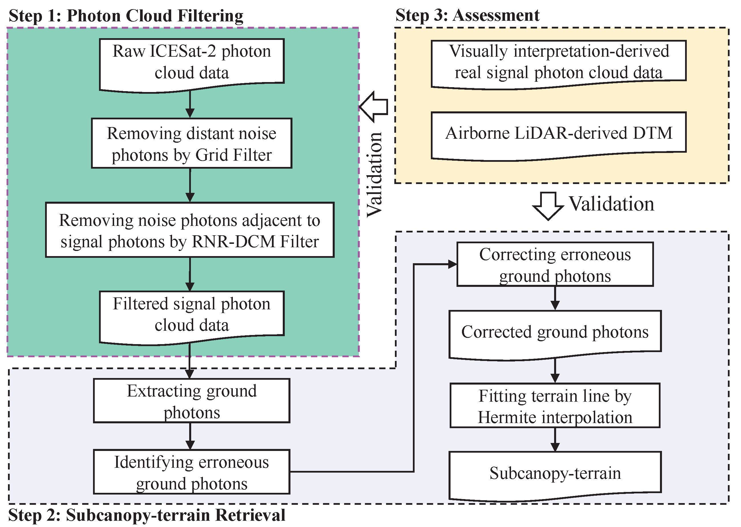
Figure 3.
Schematic diagram of DCM. (a) Photon cloud data; (b) sample of noise photons adjacent to signal photons; (c) sample of signal photons.
Figure 3.
Schematic diagram of DCM. (a) Photon cloud data; (b) sample of noise photons adjacent to signal photons; (c) sample of signal photons.
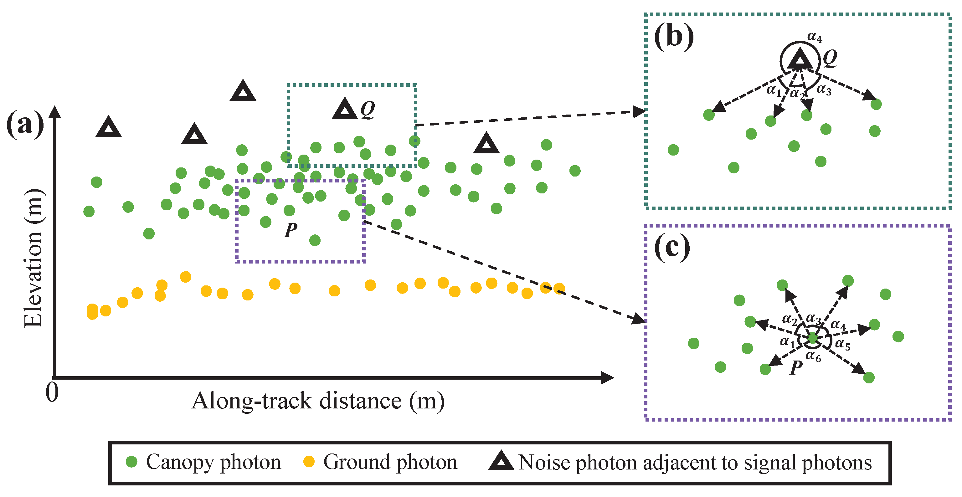
Figure 4.
Schematic diagram of sub-canopy terrain retrieval. (a) Signal photon cloud data, (b) erroneous ground photons, (c) erroneous ground photons identified by least squares fitting, and (d) erroneous ground photons corrected by percentile extraction.
Figure 4.
Schematic diagram of sub-canopy terrain retrieval. (a) Signal photon cloud data, (b) erroneous ground photons, (c) erroneous ground photons identified by least squares fitting, and (d) erroneous ground photons corrected by percentile extraction.
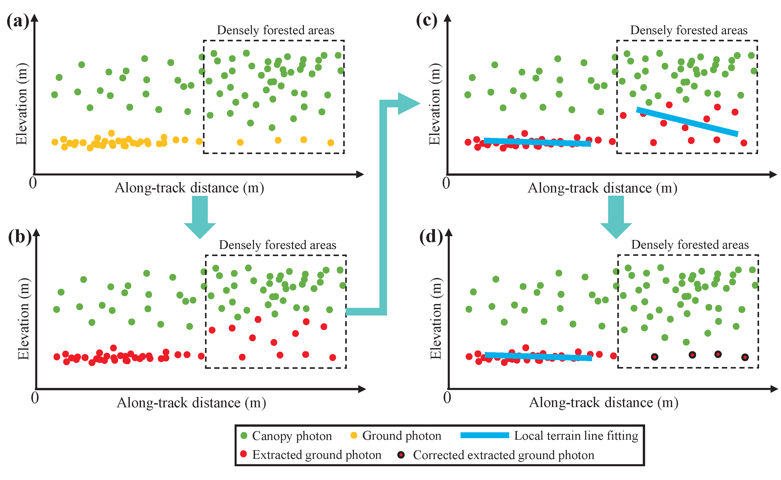
Figure 5.
Photon cloud filtering results in CA. (a,b) display the filtering result and the reference signal photons, respectively; (c,d) display the partially enlarged detail of the filtering result and the reference signal photons, respectively.
Figure 5.
Photon cloud filtering results in CA. (a,b) display the filtering result and the reference signal photons, respectively; (c,d) display the partially enlarged detail of the filtering result and the reference signal photons, respectively.
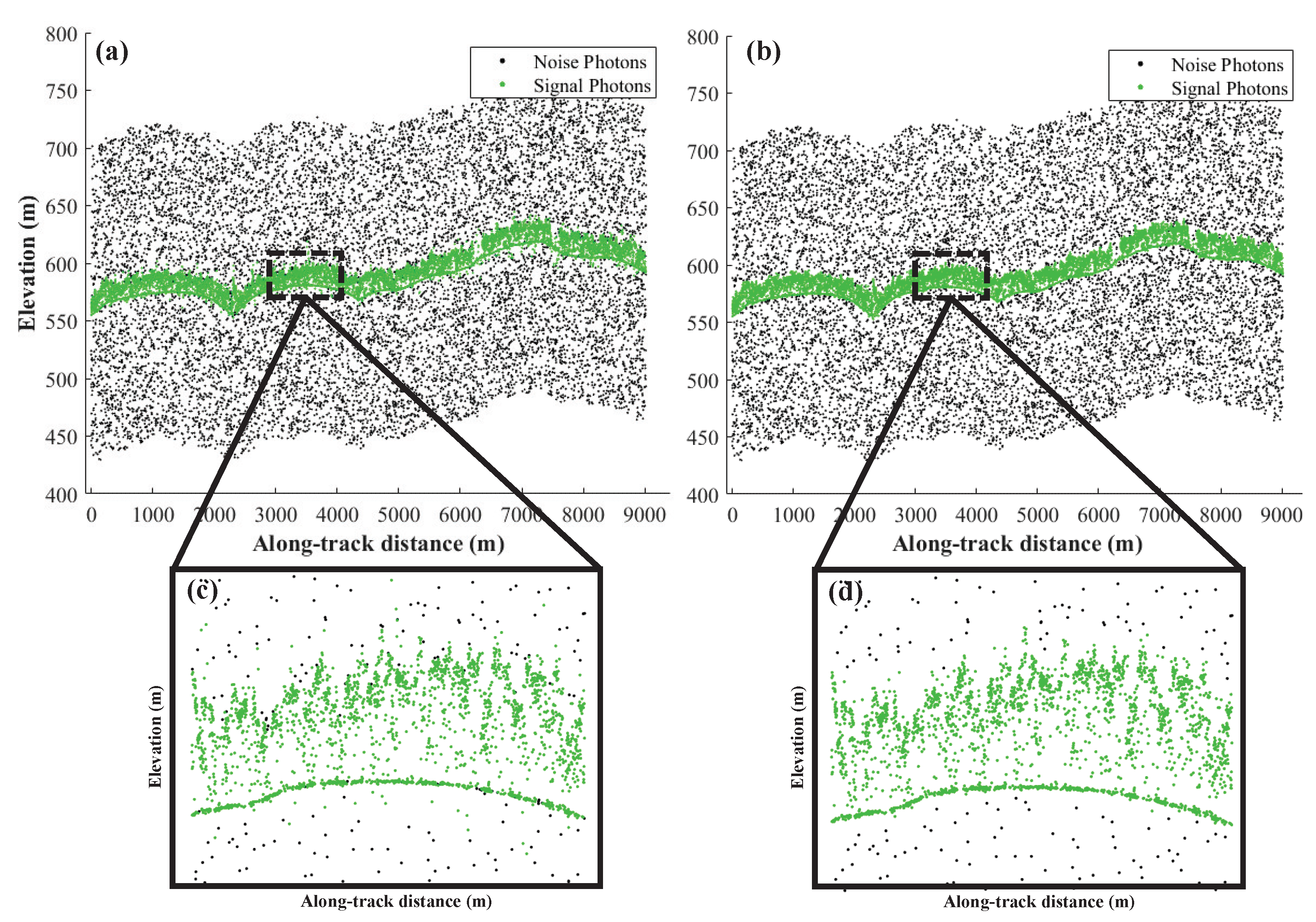
Figure 6.
Photon cloud filtering results in LD. (a,b) display the filtering result and the reference signal photons, respectively; (c,d) display the partially enlarged detail of the filtering result and the reference signal photons, respectively.
Figure 6.
Photon cloud filtering results in LD. (a,b) display the filtering result and the reference signal photons, respectively; (c,d) display the partially enlarged detail of the filtering result and the reference signal photons, respectively.
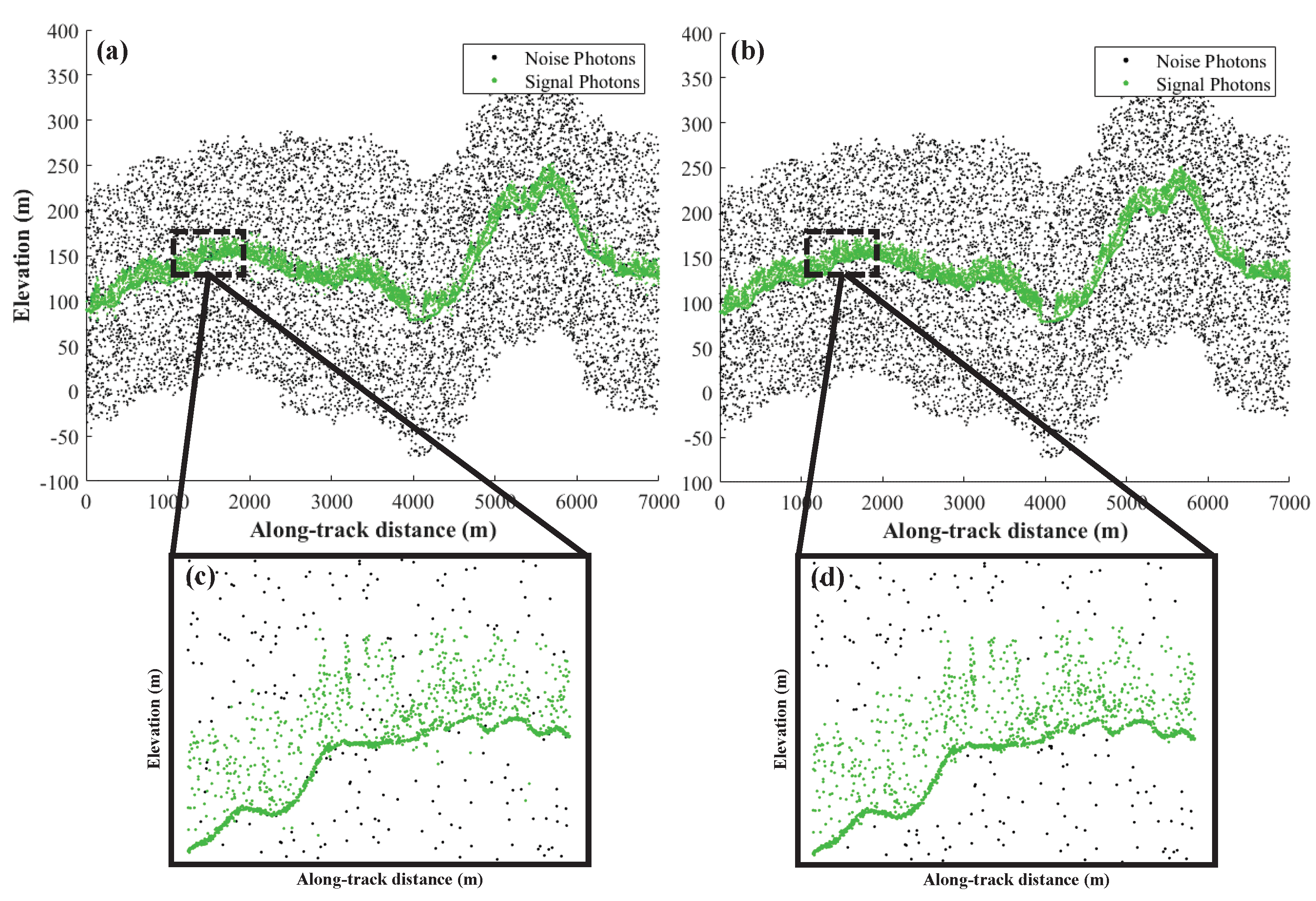
Figure 7.
Photon cloud filtering results in BOW. (a,b) display the filtering result and the reference signal photons, respectively; (c,d) display the partially enlarged detail of the filtering result and the reference signal photons, respectively.
Figure 7.
Photon cloud filtering results in BOW. (a,b) display the filtering result and the reference signal photons, respectively; (c,d) display the partially enlarged detail of the filtering result and the reference signal photons, respectively.
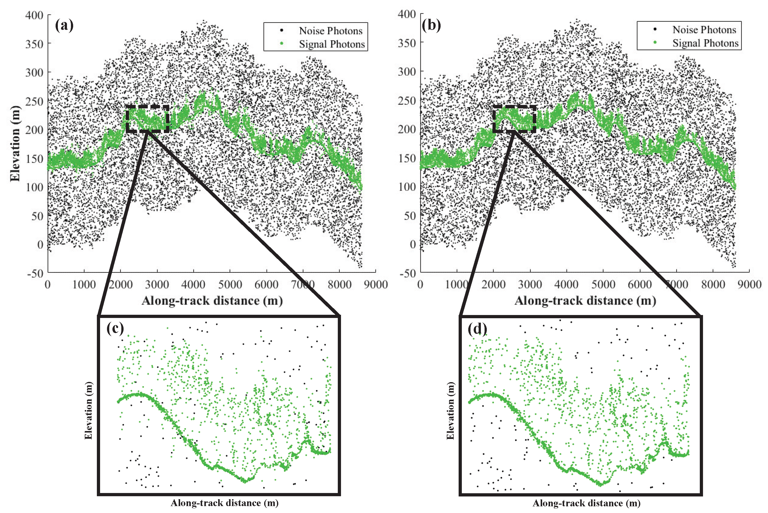
Figure 8.
Photon cloud filtering results in HARV. (a,b) display the filtering result and the reference signal photons, respectively; (c,d) display the partially enlarged detail of the filtering result and the reference signal photons, respectively.
Figure 8.
Photon cloud filtering results in HARV. (a,b) display the filtering result and the reference signal photons, respectively; (c,d) display the partially enlarged detail of the filtering result and the reference signal photons, respectively.

Figure 9.
Ground photon extraction result in BOW. (a) Extraction result, (b) unqualified partially enlarged detail of the extraction result, (c) qualified partially enlarged detail of the extraction result.
Figure 9.
Ground photon extraction result in BOW. (a) Extraction result, (b) unqualified partially enlarged detail of the extraction result, (c) qualified partially enlarged detail of the extraction result.
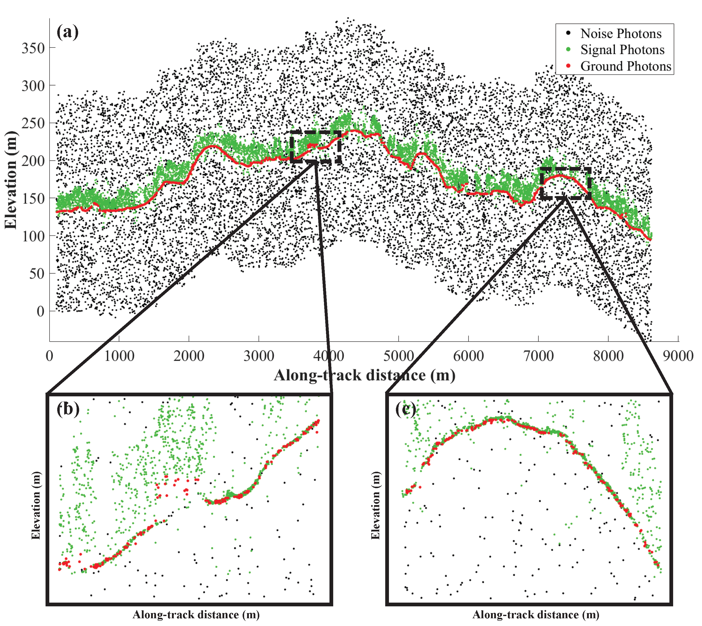
Figure 10.
Ground photon extraction result in HARV. (a) Extraction result, (b) unqualified partially enlarged detail of the extraction result, (c) qualified partially enlarged detail of the extraction result.
Figure 10.
Ground photon extraction result in HARV. (a) Extraction result, (b) unqualified partially enlarged detail of the extraction result, (c) qualified partially enlarged detail of the extraction result.

Figure 11.
Comparison between uncorrected and corrected ground photons. (a,c) display the enlarged part of uncorrected ground photons in BOW and HARV, respectively; (b,d) display the enlarged part of corrected ground photons in BOW and HARV, respectively.
Figure 11.
Comparison between uncorrected and corrected ground photons. (a,c) display the enlarged part of uncorrected ground photons in BOW and HARV, respectively; (b,d) display the enlarged part of corrected ground photons in BOW and HARV, respectively.
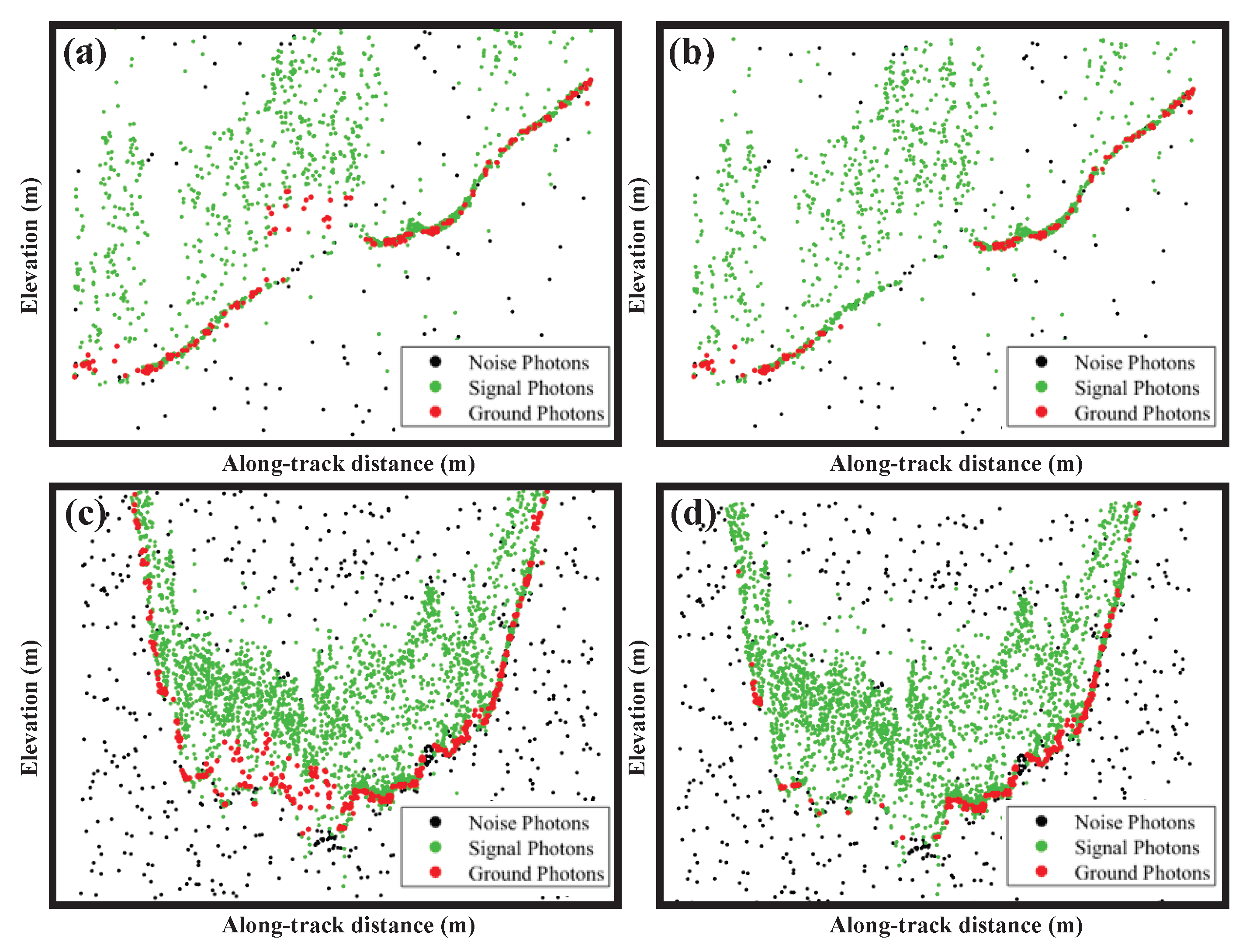
Figure 12.
Scatterplots of corrected versus uncorrected ground photons. (a,c) display the scatterplots of uncorrected ground photons in BOW and HARV, respectively; (b,d) display the scatterplots of corrected ground photons in BOW and HARV, respectively.
Figure 12.
Scatterplots of corrected versus uncorrected ground photons. (a,c) display the scatterplots of uncorrected ground photons in BOW and HARV, respectively; (b,d) display the scatterplots of corrected ground photons in BOW and HARV, respectively.

Figure 13.
Comparison between uncorrected and corrected terrain lines. (a,c) display the uncorrected terrain lines in BOW and HARV, respectively; (b,d) display the corrected terrain lines in BOW and HARV, respectively.
Figure 13.
Comparison between uncorrected and corrected terrain lines. (a,c) display the uncorrected terrain lines in BOW and HARV, respectively; (b,d) display the corrected terrain lines in BOW and HARV, respectively.

Table 1.
Detailed information about ICESat-2 data in the study areas.
| Study Area | Region | Granule ID | Latitude |
|---|---|---|---|
| CA | CAR | ATL03_20190414053207_02440301_001_01/gt3l | 6.38N–6.46N |
| LD | USA | ATL03_20190407114719_01410302_002_01/gt1l | 43.23N–43.32N |
| BOW | USA | ATL03_20190407114719_01410302_002_01/gt3l | 43.07N–43.15N |
| HARV | USA | ATL03_20190411113900_02020302_003_01/gt2l | 42.43N–42.52N |
Table 2.
Overall quantitative statistics of the proposed filtering method.
| Region | R | P | F | OA | TP | FP | FN | TN |
|---|---|---|---|---|---|---|---|---|
| CA | 0.973 | 0.985 | 0.979 | 0.975 | 18,376 | 280 | 511 | 11,984 |
| LD | 0.962 | 0.985 | 0.974 | 0.967 | 15,955 | 242 | 626 | 9124 |
| BOW | 0.963 | 0.983 | 0.973 | 0.965 | 22,118 | 390 | 846 | 11,887 |
| HARV | 0.959 | 0.985 | 0.972 | 0.961 | 26,018 | 385 | 1115 | 10,605 |
Disclaimer/Publisher’s Note: The statements, opinions and data contained in all publications are solely those of the individual author(s) and contributor(s) and not of MDPI and/or the editor(s). MDPI and/or the editor(s) disclaim responsibility for any injury to people or property resulting from any ideas, methods, instructions or products referred to in the content. |
© 2023 by the authors. Licensee MDPI, Basel, Switzerland. This article is an open access article distributed under the terms and conditions of the Creative Commons Attribution (CC BY) license (https://creativecommons.org/licenses/by/4.0/).
Share and Cite
MDPI and ACS Style
Wu, Y.; Zhao, R.; Hu, Q.; Zhang, Y.; Zhang, K. Retrieving Sub-Canopy Terrain from ICESat-2 Data Based on the RNR-DCM Filtering and Erroneous Ground Photons Correction Approach. Remote Sens. 2023, 15, 3904. https://doi.org/10.3390/rs15153904
AMA Style
Wu Y, Zhao R, Hu Q, Zhang Y, Zhang K. Retrieving Sub-Canopy Terrain from ICESat-2 Data Based on the RNR-DCM Filtering and Erroneous Ground Photons Correction Approach. Remote Sensing. 2023; 15(15):3904. https://doi.org/10.3390/rs15153904
Chicago/Turabian StyleWu, Yang, Rong Zhao, Qing Hu, Yujia Zhang, and Kun Zhang. 2023. "Retrieving Sub-Canopy Terrain from ICESat-2 Data Based on the RNR-DCM Filtering and Erroneous Ground Photons Correction Approach" Remote Sensing 15, no. 15: 3904. https://doi.org/10.3390/rs15153904
Note that from the first issue of 2016, this journal uses article numbers instead of page numbers. See further details here.