


Satellite-Based Identification and Characterization of Extreme Ice Features: Hummocks and Ice Islands

1
C-CORE, Ottawa, ON K2K 2A4, Canada
2
C-CORE, St. John’s, NL A1B 3X5, Canada
*
Author to whom correspondence should be addressed.
Remote Sens. 2023, 15(16), 4065; https://doi.org/10.3390/rs15164065
Submission received: 30 June 2023
/
Revised: 3 August 2023
/
Accepted: 7 August 2023
/
Published: 17 August 2023
(This article belongs to the Special Issue Recent Advances in Sea Ice Research Using Satellite Data)
Abstract
:The satellite-based techniques for the monitoring of extreme ice features (EIFs) in the Canadian Arctic were investigated and demonstrated using synthetic aperture radar (SAR) and electro-optical data sources. The main EIF types include large ice islands and ice-island fragments, multiyear hummock fields (MYHF) and other EIFs, such as fragments of MYHF and large, newly formed hummock fields. The main objectives for the paper included demonstration of various satellite capabilities over specific regions in the Canadian Arctic to assess their utility to detect and characterize EIFs. Stereo pairs of very-high-resolution (VHR) imagery provided detailed measurements of sea ice topography and were used as validation information for evaluation of the applied techniques. Single-pass interferometric SAR (InSAR) data were used to extract ice topography including hummocks and ice islands. Shape from shading and height from shadow techniques enable us to extract ice topography relying on a single image. A new method for identification of EIFs in sea ice based on the thermal infrared band of Landsat 8 was introduced. The performance of the methods for ice feature height estimation was evaluated by comparing with a stereo or InSAR digital elevation models (DEMs). Full polarimetric RADARSAT-2 data were demonstrated to be useful for identification of ice islands.
1. Introduction
An extreme ice feature (EIF) is an ice feature that could cause an extreme design load on an offshore platform from a fixed-structure point of view, ice scouring seafloor facilities or significant ship damage. EIFs include rubble fields, ridges, hummocks, stamukhi, icebergs, ice islands and multiyear (MY) floes. An ice ridge is a line or wall of broken ice forced up by pressure [1]. A rubble field is an area of many ridges with similar characteristics. Multiyear ice floes (pieces of ice 20 m or more across) are old ice floes that have survived at least two summers’ melt and are much thicker (up to 4 m and more [2]) than younger ice. Stamukhi are pileups of deformed sea ice that are grounded to the sea floor and are found in shallow water. A hummock is defined [1] as a hill of broken ice that has been forced upward by pressure. The hummock field can produce significant seabed gouging (up to 3.5 m in depth), fragmented during the grounding process [3]. The presence of EIFs in the Canadian Arctic has been a topic area of interest for many years with records available starting from 1946 [4]. EIFs in the Beaufort are most likely to occur along the northwest edge of the Queen Elizabeth Islands and in the pack ice of the Arctic Ocean [5]. More recently, the warming Arctic appears to have affected both the occurrence and characteristics of these ice features. With the increasing impact of climate change, the hazardous ice features remain a threat to stationary and mobile infrastructure in the southern Beaufort Sea [6] because of the increased frequency and relative velocities of certain ice hazards [7].
Ice islands are generated as a result of calving from glaciers and ice shelves that are present along the east coast of Canada and the Beaufort Sea. The size of the ice islands may be up to 1000 or more square miles and their thicknesses up to 75 m. In the Beaufort Sea, ice islands are large tabular icebergs that calve from the ice shelves located along the northern coasts of Ellesmere and Axel Heiberg islands and drift into the Arctic Ocean where they circulate in a clockwise direction for many years [5]. Although definitions vary, ice islands can also be described as any tabular icebergs whose waterline lengths range from hundreds of meters to many kilometers, generally have freeboards under 20 m and an overall thickness of up to 55 m [8]. However, Beaufort Sea ice islands generally have maximum dimensions of tens of meters or smaller. Beaufort Sea ice islands predominantly come from Ellesmere Island ice shelves, which are a combination of fresh and salt water ice formed from snowfall and sea-ice accretion. The low freeboards of ice islands make them challenging to detect and their low drafts allow them to pass over continental shelf areas.
For decades, upward-looking sonar have been used to study ice in the Beaufort Sea, and for the last 30 years, satellite imagery have been used to report on surface ice conditions. One of the first remote sensing studies to detect EIFs was conducted by Pilkington et al. [5], who used satellite imagery and concluded that a spatial resolution of at least 15 m on both radar and optical is required for detecting EIFs with 500 m diameters. By comparing RADARSAT-1 and Quickbird images [9], it was concluded that RADARSAT-1 Extended High images were best at detecting ice features. Fine-mode images provided more details, but it was difficult to identify new features in the data. Quickbird images provided exceptional detail, but clouds and darkness were severe limitations. Rubble fields were difficult to detect during freeze-up and in land-fast ice, but they could be characterized using satellite SAR. During break-up, grounded rubble fields would persist after other ice had melted and it was possible to detect them even with RADARSAT-1 ScanSAR imagery. Work by [9] indicated that RADARSAT-1 fine-mode data with 8 m resolution were good at characterizing but not identifying many ice features of interest. The best resolution to detect EIFs was RADARSAT-1 Extended High with 18 to 27 m resolution. Studies have been carried out with multiple SAR acquisition frequencies, but other differences in imaging parameters make it difficult to make definitive conclusions regarding the preferred frequency band. Comparisons between C-band and L-band data [10] indicated that L-band data had better contrast between deformed and level ice and tended to image the full extent of deformation, whereas only select parts of the deformation were visible in C-band. There are many operational SAR sensors at various frequencies and polarizations. The systems reviewed in paper [10] are suitable for EIF monitoring, but there are trade-offs for their use. The current trends of increasing air temperature at northern high latitudes have been at more than twice the rate of the global average since the middle of the 20th century. Climate warming has significant impacts on northern infrastructure, hydrology and ecosystems, precipitation and snow depth and the global climate [11]. Radar backscattering properties can be extremely sensitive to the freeze/thaw states of the surface [12]. Snow cover, especially wet snow, may influence SAR backscatter, including polarimetric scattering mechanisms [13,14]. Therefore, the interpretation of SAR signals from targets with variable dielectric properties can be limited without understanding the actual scattering processes.
In a study conducted by Canatec [15], ENVISAT 30 m data were utilized along with RADARSAT-2 fine-mode data (8 m) for distinguishing small features. Only some of the data sources were of sufficient resolution to detect such targets. ENVISAT and RADARSAT-2 Wide (both 30 m resolution) were suitable for targets that covered 2–3 pixels. RADARSAT-2 ScanSAR Wide (100 m resolution) and MODIS (240 m resolution) were too coarse to detect targets of the minimum size. RADARSAT-2 ScanSAR Wide imagery could not clearly identify MY floes because of its resolution, despite several “bright returns” from locations known to contain MY ice.
Aerial and satellite SAR sensors are capable of collecting data with multiple polarizations. With full polarimetric data, it is possible to resolve the unique signatures associated with particular radar scattering mechanisms related to different surface features. Therefore, full polarimetry offers, in principle, a means of discriminating between different ice features in terms of physical properties that generate these unique scattering processes. Polarimetric decompositions have been used to identify three types of FY sea ice (i.e., deformed ice, rough ice and smooth ice) and wind-roughened open water [16]. Work by [17] demonstrated the capabilities of detecting icebergs in sea ice using polarimetric decompositions by relating the dominant volume scattering mechanism to glacial ice.
Ice ridges and icebergs pose a major threat to both ships and offshore facilities, and these features have to be considered for structural design loads on a ship hull [18]. Satellite observations can be used for sea ice ridge identification and characterization [19,20,21]. Icebergs in open water have been operationally monitored with SAR satellites over the last two decades [22,23].
In the past, various studies have been undertaken to address the presence of EIFs in the Beaufort Sea, including their impact frequencies, sizes and thicknesses. Ice features that fit into this category include large ice islands and ice-island fragments, rubble fields, multiyear hummock fields (MYHF) and other EIFs, such as fragments of MYHF and large, newly formed hummock fields.
Airborne electromagnetic surveys [24] enabled observations of the thickness of different sea ice types and EIFs in the Canadian Beaufort Sea. In the seasonal ice zone, there are regions with heavily deformed ice thicker than 10 m, and occasional multiyear hummock fields of similar thicknesses occur. Satellite data cannot directly measure EIF thickness, although it is possible to measure the freeboard (height above water surface) of ice floes [25] and icebergs in open water [26] using radar altimetry. Single, very-high-resolution (VHR) electro-optical satellite images can be used to estimate the height of ice features from shadows [27]. The usage of stereo VHR electro-optical images enable extraction of sea-ice and iceberg topography, which can potentially serve as an indicator of ice feature thickness. The advanced single-pass interferometric capability of TerraSAR-X/TanDEM-X (TDM) satellites can also be used to extract sea-ice local surface topography [28] and iceberg topography [29]. A comparison of a digital elevation model (DEM) extracted from stereo VHR electro-optical images with a DEM based on TDM InSAR [30] demonstrated also the possibility to detect icebergs in sea ice with high accuracy, which is an important practical task.
The goal of this paper is to investigate and demonstrate possibilities of identification and characterization of EIFs in the Canadian Arctic using satellite data. The focus will be on hummocks and ice islands because they pose significant risks for offshore infrastructure. We will use VHR electro-optical, Landsat-8, RADARSAT-2 and TDM data to demonstrate the feasibility of achieving this goal. Portions of the Canadian Arctic are ice covered for much of the year and EIFs can persist for several years. Developing tools that automate the process of identifying EIFs can be used to develop an inventory of hazardous features that can be used for risk management for transportation or other marine operations in the area.
2. Study Area and Data
2.1. Study Areas
The main study areas were in the Canadian Arctic, specifically the Beaufort Sea and Baffin Bay. Based on many years of C-CORE monitoring experience, these areas were selected as having high probability for EIF locations. Also, the Beaufort Sea is largely a closed sea and extreme ice features in the area tend to persist for several years. There is an interest in developing an inventory of this region, to assess the risk they pose for transportation and resource exploration. VHR, medium- and low-resolution electro-optical and infrared data including Landsat 8 and moderate-resolution imaging spectroradiometer (MODIS) were used for research. VHR and medium-resolution SAR and VHR electro-optical and infrared satellites were tasked over areas of the Lincoln Sea, Meighen Island, Baffin Bay, Axel Heiberg, Prince Patrick and Borden Islands. Figure 1 shows all sub-areas that were monitored.
2.2. Satellite Data
In 2013–2014, 84 RADARSAT-2 (RS-2), 10 TerraSAR-X (TSX) and 8 COSMO-SkyMed (CSK) images were acquired. One GeoEye-1 image (Copyright of DigitalGlobe, presently it is MAXAR Technologies) was acquired over Meighen Island in September 2013, one SPOT-6 (Copyright of Airbus Defence an dSpace) mono image over Prince Patrick Island and three SPOT-6 stereo pairs over Borden Island in April of 2014. During the analysis, 40+ Landsat 8 and MODIS images were also analyzed. In addition, 32 TDM single-pass InSAR pairs and one Pléiades stereo pair were acquired over Baffin Bay in 2016. One stereopair of WorldView-2 (Copyright of DigitalGlobe, presently it is MAXAR Technologies) and 17 TDM InSAR pairs (Copyright of DLR) over sea ice near the Axel Heiberg Island in 2014. For the images used in the following figures, the specific image acquisition dates are provided.
2.3. Validation Information
The collection of field measurements in the Arctic was not performed under our project. However, the validation of the DEM extraction methods are often performed by inter-comparison with DEMs extracted by other techniques, for example, airborne stereo photo or lidar [31,32]. The results of single-pass TDM InSAR DEM validation with ICESat data show that the absolute height errors of the TDM DEM are small, mostly on the order of 1–2 m [33]. A comparison of TDM InSAR DEM for various landcover classes with airborne lidar shows relative accuracy between 1.9 and 5.9 m [34]. A similar relative height error of 2 m was reported [35] for the production of global TDM DEM based on the comparison with laser scanning DEMs, SRTM data and ICESat points. The method of height from shadow was used to measure the great pyramid in Giza by observing the length of the shadow in the 6th century B.C. [36]. It was used with optical satellite data for ridge height estimation [27,37] and for building height estimation with validation showing the absolute error within 1.24 m–3.76 m [38]. The problem of building height extraction from VHR and high-resolution SAR images was extensively investigated and several solutions have been proposed [39,40,41,42,43]. The height retrieval accuracy was evaluated using ground data and lidar digital surface model and was dependent on SAR resolution [40]. For spotlight (1 m resolution) TerraSAR-X images, the mean absolute height errors varied between 1 and 3.4 m, and the standard deviation of height errors were between 1.3 and 5.8 m depending on type of the buildings (primarily, roof shape).
3. Methods and Results
3.1. Electro-Optical and Infrared
3.1.1. VHR Data
Very-high-resolution (VHR) satellite imagery is now approaching the quality of airborne observations, which were used for many decades for sea-ice reconnaissance [1,44]. Imagery acquired by VHR optical satellites can be used for qualitative image interpretation to identify various sea-ice features and is especially valuable when detailed ground validation is not available. Optical imagery has been used to map pressure ridges to verify bright features in SAR images [45], and imagery acquired by a VHR airborne camera were used for the operational planning of navigation through drifting ice [46]. An overview of the retrieval from VHR satellite imagery of five sea-ice parameters including melt pond coverage, open water fraction, ridge height, floe size and openings and closings [37]. Thus, an expert can easily identify EIFs in a VHR image. Brian Wright, who had many years of expertise with EIFs in the Beaufort Sea and other areas, was consulted to assist in interpreting VHR satellite data and detecting EIFs.
Ice islands in the Beaufort Sea appear “striped” in optical imagery and are more visible in winter when the snow is dry. One defining characteristic, along with their enormous size and tabular shape, is the rolling terrain of almost parallel hills and troughs of similar size and depth. Hills are typically parallel to prevailing wind direction and shore. The ridges of multiyear land-fast sea ice also give a striped appearance, but of a smaller scale than those of ice islands/ice shelves [47]. A typical ice island has a convex, wavy surface and is usually smoother than the surrounding ridged sea ice (Figure 2). Ice-island fragments are similar to ice islands but have two main differences. First, ice-island fragments have smaller sizes (we considered their size to be less than 100 m). Second, they very often appear as small features with sharp edges.
The appearance of hummocks, including MYHFs, in VHR electro-optical and infrared images is provided in the following sections.
3.1.2. Stereo-Photogrammetry
Ice islands and their fragments rise up to 10 m above the ocean surface, and this freeboard may be captured by any remote sensing technology capable of extracting 3D information (topography) at high resolution. The most common satellite-based method of extracting a digital elevation model (DEM) (a 3D representation of a terrain’s surface elevations) is the stereo-photogrammetric method. In addition, the method called height from shadow [48] can be useful to validate the DEM height of ice features [27].
Stereo datasets acquired by VHR optical and SAR satellites were analyzed. Stereo SPOT 6 imagery was acquired over Axel Heiberg Island. Stereo images allow sea-ice topography to be estimated after extracting DEM. For a sea-ice environment that also includes a snow layer, the DEM includes the snow surface and may also be referred to as a digital surface model (DSM). PCI Geomatica Orthoengine (now called CATALYST Professional) and the ERDAS photogrammetric module were used to generate the DEM.
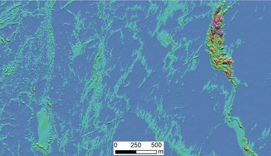
Testing different software parameters on SPOT 6 stereo images demonstrated that a DEM of sea ice and large icebergs can be extracted. DEM generation over ice fields in the Canadian Arctic with along-track SPOT5 HRS stereo data has previously been described in [31]. The results demonstrated that stereoscopy can perform well over ice and snow-covered surfaces. The DEM accuracy is acceptable for estimating the relative elevation of extreme ice features with respect to each other or the surrounding ice, but to estimate absolute elevation with respect to sea surface height, ground control points (GCPs) must be collected. Figure 3a shows SPOT 6 imagery (acquired on 27 April 2014) over EIFs including ice islands, ice-island fragments, ridges, new forming hummocks and MYHFs. Figure 3b shows an example DEM corresponding to an area in the SPOT 6 imagery. It can be seen that the height over the ice surface (including snow) of hummocks varies from 3 to 4 m for MYHF and up to 25m for forming hummocks. The height of ice islands is about 5 to 7 m, which is consistent with the freeboard of Ward Hunt Island, where many of the ice islands are expected to originate from. The DEM is a valuable source of ground-truth information for EIF analysis.
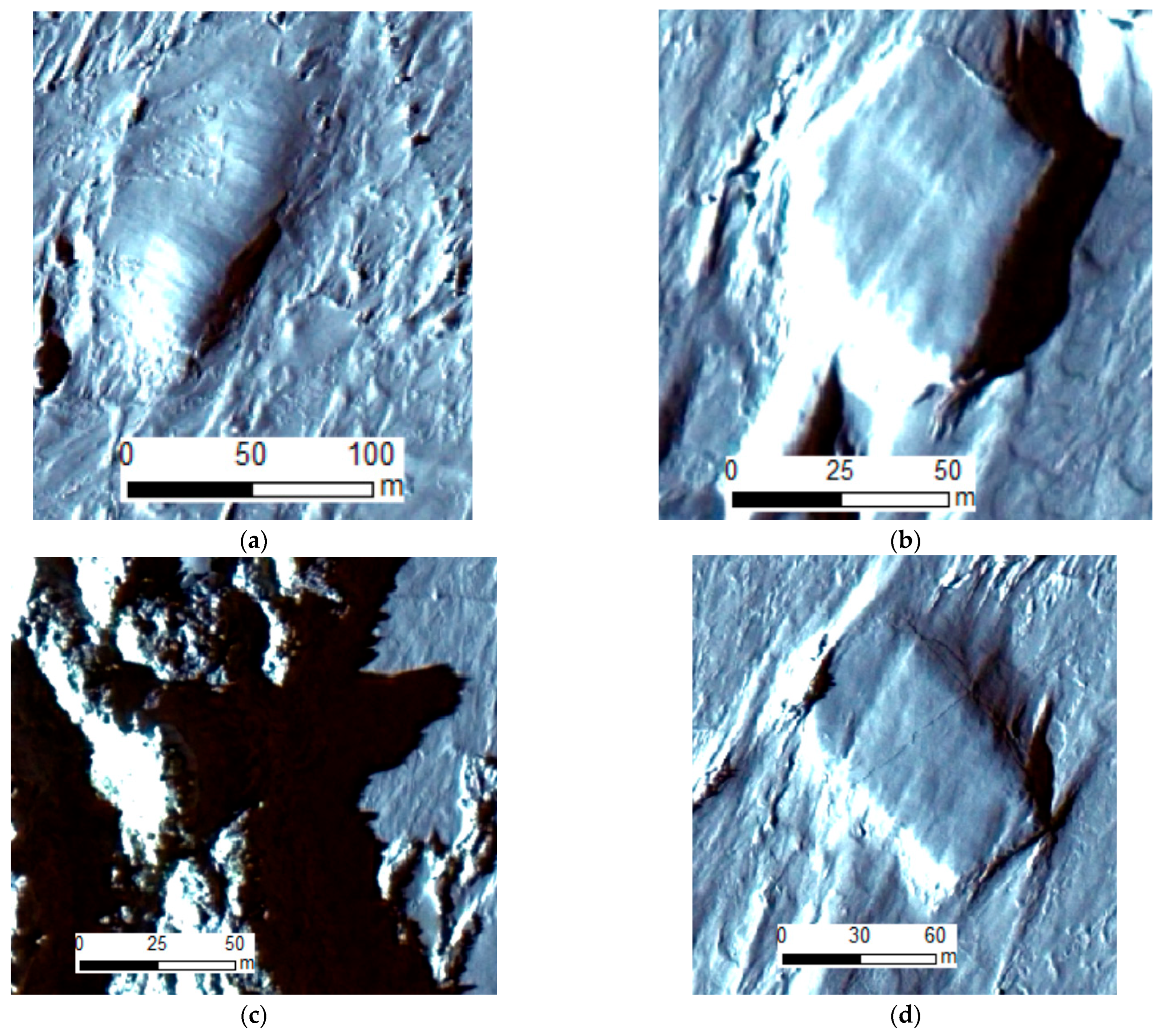
Stereo imagery and the produced DEM were analyzed to understand the maximum height and possible thickness of EIFs, which allows for better EIF identification and quantitative characterization. The height information provided by a DEM is useful for identifying smaller EIFs. For example, the small MYHF in Figure 4 appears to be similar to the rubble field of Figure 4c in the WorldView-2 image (acquired on 29 April 2014). However, using the DEM, these features can be clearly distinguished because MYHFs have higher freeboard than rubble fields (compare Figure 4b with Figure 4d). The height of MYHF above the sea surface (including snow) spans from 2 m to 4 m (Figure 4b), whereas a rubble-field elevation (Figure 4d) varies from 0 m to a maximum of 1.6 m (the mean is below 1 m).
A DEM is used as an additional source of ground-truth (verification) information for EIF identification and can also be used to generate a topographic map of sea ice and snow surface.
3.1.3. Height from Shadow
In sunny and cloud-free conditions, all features protruding from the level ice surface produce shadow. The method for height estimation using a single high-resolution image is to analyze the ice-feature shadow, which is dependent on the orientation of the feature. The developed algorithm [27] facilitates the extraction of ice-feature height from shadow and the deriving of statistical information on ice deformation parameters.
In the work [49], a vertically downward-looking camera mounted on a helicopter was used to collect photographs with ground resolutions of 0.5–0.8 m. The ice-feature height H was calculated from the measured shadow length (Figure 5) and from knowing the sun elevation angle as
However, the approach described by Equation (1) cannot be applied to satellite imagery, which is collected from different angles (e.g., elevation angle for our GeoEye-1 image is 74.57°).
The height can be derived from the shadow considering image-acquisition geometry without utilizing the rational polynomial coefficient (RPC) and the sensor (camera) model [50]. In this method, the height, H, was calculated as
where is the azimuth angle of the sun; is the elevation angle of the sun; and are the azimuth and the elevation angles of the satellite, respectively (Figure 5a); and is the measured distance between the image of the top of the ridge and the shadow (Figure 5b).
Equation (2) was applied to analyze the height of different ice features using height-from-shadow techniques and to compare the height to DEM. Figure 6 shows a WorldView-2 image containing ice-island fragments. The red line over the edge of the fragment was used for height estimation. The stereo DEM of these ice-island fragments was compared to the height profile in Figure 6 (bottom) extracted using Equation (2) along the shadow base. It can be seen that the height from shadow provides a height estimate of about 3.5 to 4 m. Similar height values can be found in the DEM for this ice-island fragment. The quantitative comparison between these two techniques can be found in paper [27].
More EIF (ice-island fragments and forming hummocks) shown in Figure 7 were also investigated with the height-from-shadow method, and the results were compared to stereo DEM (Table 1). The comparison shows good agreement between the two methods. The error of height estimation for ice-island fragments is about 5–10% but about 15% for the hummock peak.
3.1.4. Landsat 8
Pansharpened Image
Landsat 8 measures different ranges of frequencies (bands) along the electromagnetic spectrum. Among 11 bands, we used the panchromatic band (0.500–0.680 µm) with 15 m resolution to pansharpen the 30 m resolution RGB color composite image.
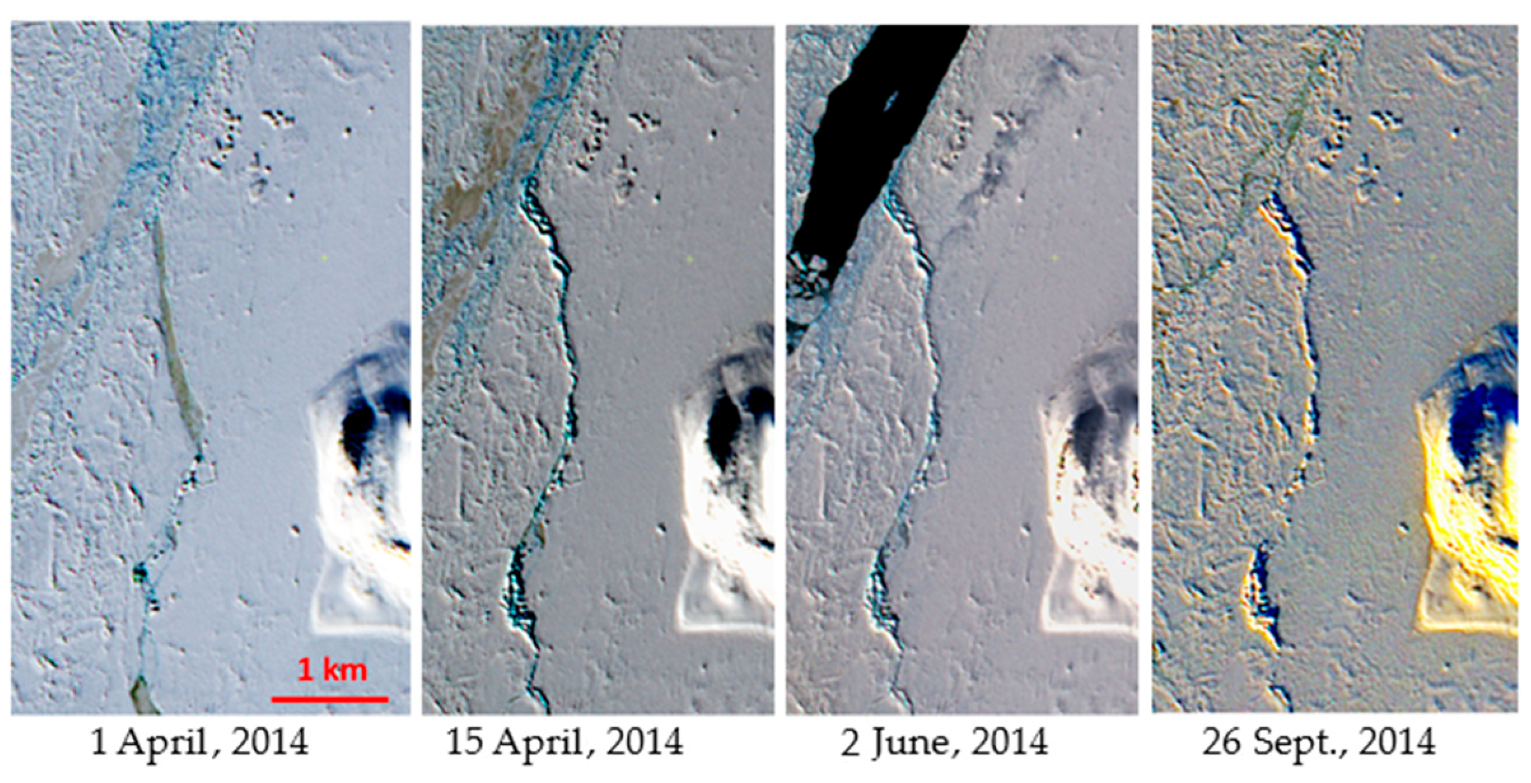
Figure 8 shows the forming process of hummocks near Axel Heiberg Island. A fragment of one stereo SPOT 6 image and DEM over the same area is shown in Figure 3.
EIFs have certain properties that allow each feature to be detected and identified in optical imagery. First of all, MYHF and ice islands are much thicker than the surrounding sea ice. When a feature protrudes from the ice surface it creates brightness (intensity) variation in the image because of shadow and its bright pattern generated from the feature side oriented toward the sun. Another reason for brightness variation is that very often the EIF surface may have different roughness from other sea ice. The intensity variation in optical satellite imagery appears as texture, which is very often a specific property for certain EIFs. However, multiyear floes and rubble fields may have similar textures resulting in an ambiguity in feature identification when only the visible bands of optical images are used. A stereo DEM was used as an additional source of ground-truth information, which is a good indicator of EIF thickness.
Thermal Infrared
Landsat 8 has two thermal infrared (TIR) bands of 100 m resolution: Band 10 with the range of 10.6 to 11.2 µm and Band 11 with the range of 11.5 to 12.5 µm.
For detecting EIFs in Landsat 8 imagery, a new method can be introduced that utilizes the TIR band for improving the identification of thicker ice features. The improvement is possible because thicker features have colder temperatures than the surrounding sea ice and appear dark and have the contrast from other ice features in the thermal image. The Landsat 8 thermal band has the following main limitations for identifying EIFs:
- A coarse resolution (100 m);
- Sensitivity to the presence of even small amounts of cloud;
- Missing thermal contrast variation for the ice area at the edge of sea ice and open water;
- Thermal contrast may be caused by other features; in some cases thermal contrast was observed from multiyear floes and land-fast ice features;
- In the summer months, when snow is wet or ice is covered by melt pounds, the thermal band may not generate sufficient contrast for automated detection of thicker features.
The following Figure 9 shows the typical appearance of EIFs in VHR imagery, a stereo DEM, and visible and thermal bands of Landsat 8.
In optical-imagery ice islands have brighter and darker sides (Figure 9a,c) because of variation of the local sun-incidence angle. Ice-island thickness, as shown in Figure 9b, is a major factor that facilitates its identification. The same ice island can be identified in Landsat 8 using the visible (Figure 9c) and thermal (Figure 9d) bands.
Ice-island fragments are similar to ice islands, but they are much smaller. The thermal signature in Landsat 8 can be visible only when there is a cluster of fragments shown as dark areas because the resolution (100 m) of the thermal band in many cases is coarser than the size of an individual fragment. Absence of thermal contrast may lead to missing individual fragments with automated detection.
MYHFs can be identified based on textural information in combination with thermal contrast (Figure 10). As shown in Figure 10b, MYHFs are thicker than ice floes. Figure 10a–d show two MYHFs, with the larger one in the middle and the smaller one (the same as shown in Figure 4) in the top right corner. Greater thicknesses of MYHFs generate temperature difference between the MYHF and adjacent ice resulting in thermal contrast, as is shown in Figure 10d.
3.2. SAR
3.2.1. Single-Pass InSAR
The advantages of using an interferometric SAR (InSAR) method for detecting and characterizing icebergs in sea ice have been demonstrated [30]. Single-pass TanDEM-X InSAR data enable analysis of iceberg topography and detect icebergs in sea ice with a high probability of detection. The same single-pass TDM InSAR technique was applied to extract the topography of forming hummocks (Figure 11a). The TDM pair of the StripMap mode, incidence angle 43°, HH polarization and high resolution (slant range 1.2 m, azimuth 3.3 m), was acquired on December 12, 2014. The values of stereo DEM (29 April 2014), extracted from VHR WorldView-2 images, show that the height of the hummock peaks approached 25–29 m. However, the values of InSAR DEM over peaks of the same hummock is only about 18–21 m. The difference between VHR optical and InSAR DEMs of about 28% can be explained by the time difference between the SAR and optical images of more than seven months, including summer when the hummock peaks melted. Another reason for the lower values of InSAR DEM over peaks can be justified by a coarser resolution (3.3 m for TDM data vs. 0.5 m for WorldView-2 data), which makes the InSAR method less sensitive for sharp height variations.
3.2.2. Polarimetry
The polarization of a radar wave is the orientation of the electric field, and signals can be transmitted and received with multiple polarizations. Four possible linear polarizations are HH, VV, HV and VH, where the first letter refers to the transmit polarization, and the second letter refers to the receive polarization (H refers to horizontal and V to vertical).
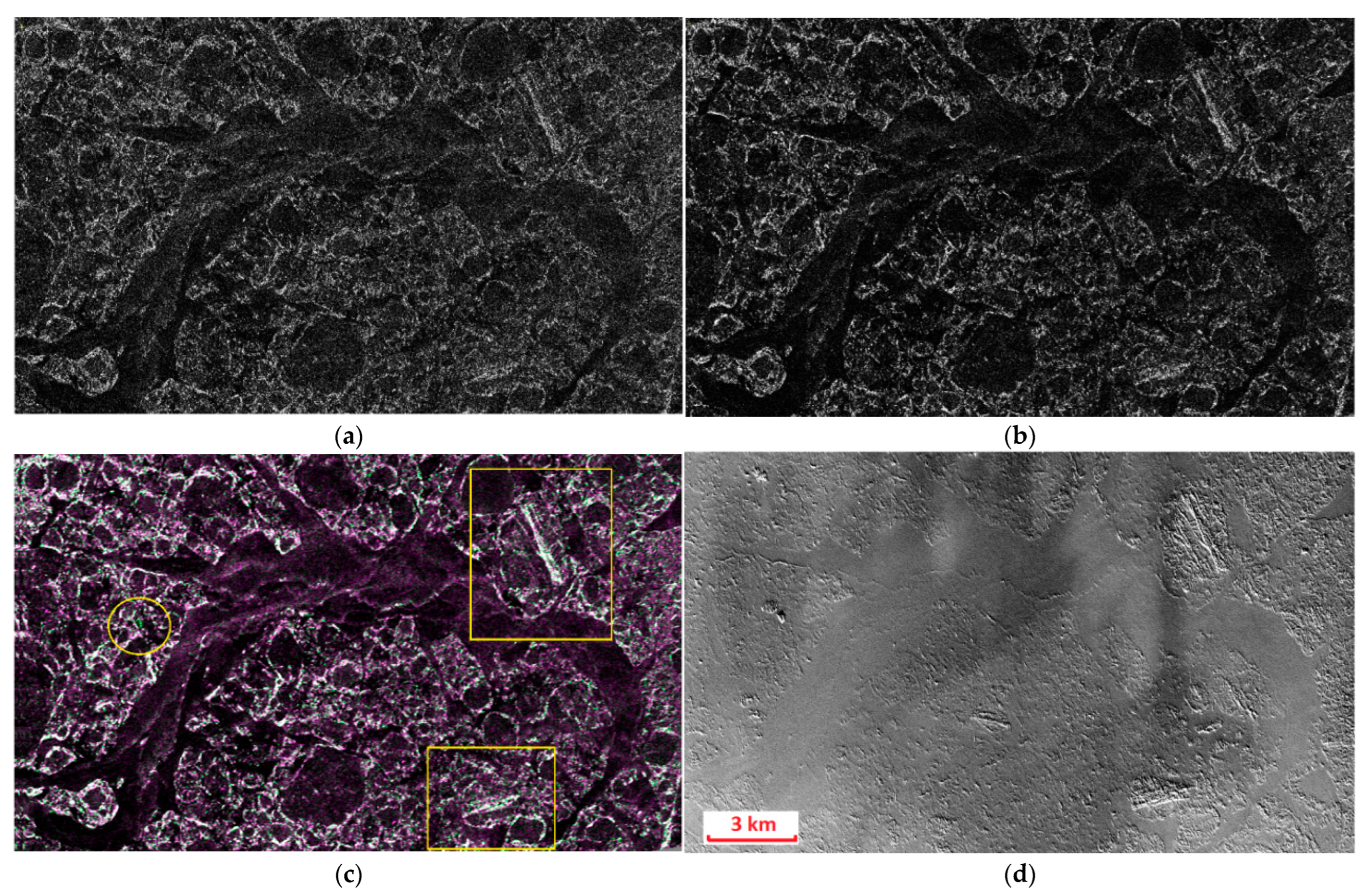
Full polarimetric data allow analysis of different scattering mechanisms through polarimetric decompositions [51]. The Pauli polarimetric decomposition, which represents three major scattering mechanisms (surface (shown in blue), volume (green) and double bounce (red)), was applied on RADARSAT-2 (RS-2) FQ data and found to be useful for indicating glacial ice (icebergs and ice islands). Icebergs were detected in a color composite image (FQ27, 26 September 2013) as green features (representing volume scattering) and highlighted by blue circles in Figure 12. It is interesting to note that glacial ice features were more readily distinguished with full polarimetric data than with single- and dual-pol data.
In addition to an FQ mode, RS-2 has an FQ Wide mode that covers 50 km by 25 km with the same resolution. Pauli decomposition was applied to an FQ20W image acquired on 7 March 2014. Since that time (September 2013), the ice has dispersed, but it can be seen that one ice island (highlighted by red circle) frozen into sea ice is still in the same place (Figure 12 (bottom)). This experiment confirms that an FQW image can also be used for the detection of glacier ice features.
Another combination of dual-pol channels of the RS-2 standard mode improved the possibilities of glacial-ice identification. Color composites of standard beams S1, S4 and S8 (incidence angles are 20, 34 and 49 degrees, respectively) were analyzed. It was found that S8 was better at identifying glacial ice than imagery acquired with lower incidence angles.
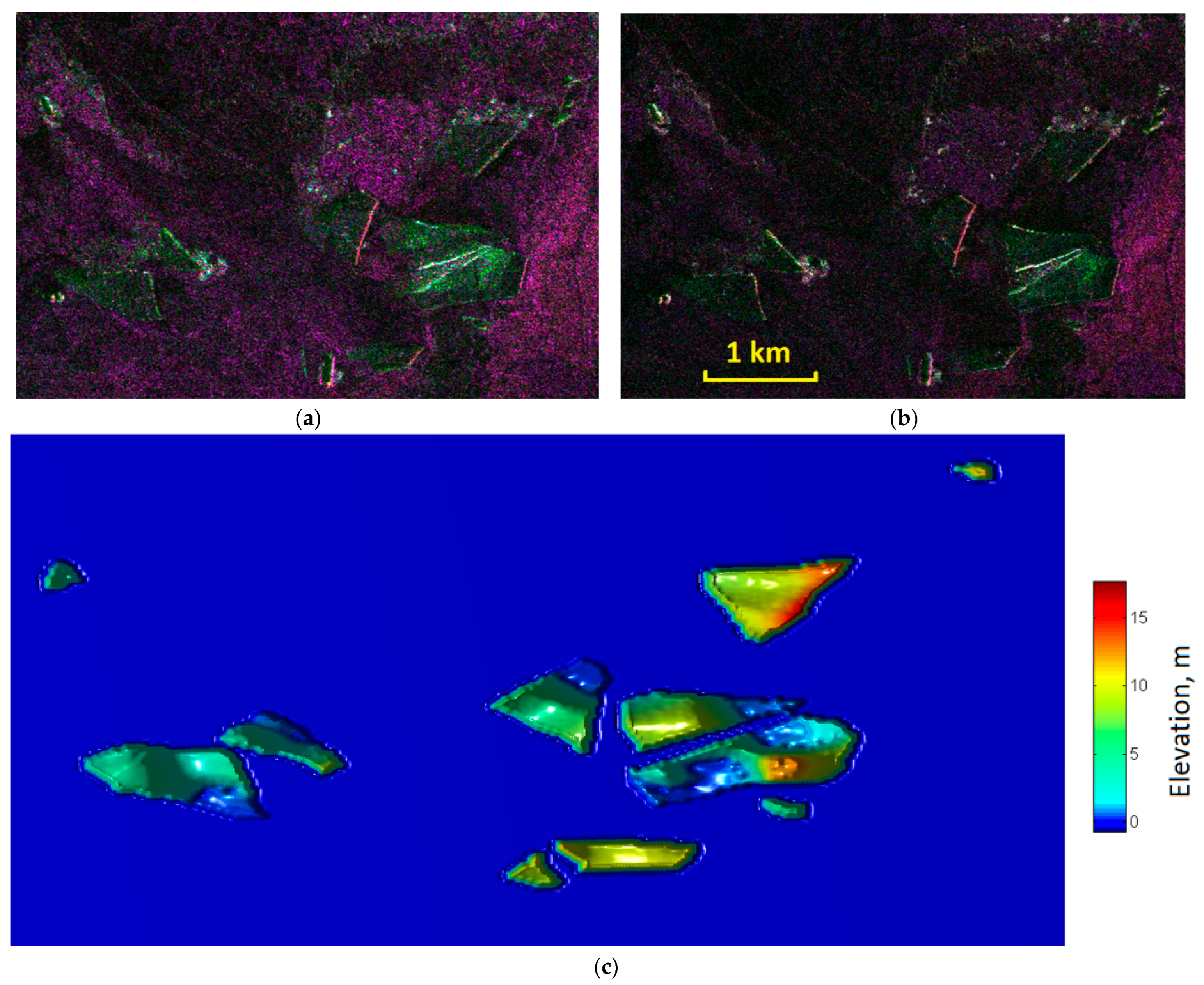
Several dual-polarized RS-2 and TSX datasets have been acquired. Various combinations of dual-polarized imagery, as well as color composites generated from both satellites, were analyzed. Color composites of dual-polarized RS-2 standard beam mode S8 imagery (acquired on 3 March 2014) are shown in Figure 13. Original radar images are HH (a) and HV (b). An RGB color composite (c) was generated from an RS-2 image as HH—red, HV—green and HH—blue. The Landsat 8 image used as verification is shown in Figure 13d. It can be seen from the Landsat 8 image that an ice island and multiyear hummock fields were present. The ice island, with a waterline length of about 370 m, can be identified in the color composite image (Figure 13). The ice island is circled in Figure 13c and is shown also on (e) and (f). Large hummocks are identified in the HV channel of the SAR image and even better in the color composite image and demonstrate how these features can be detected over large areas, as RS-2 standard images have swath coverage of 100 km. Color composites are useful for identifying band combinations and can be used in the future as the basis for automated algorithms.
3.2.3. Height from Shadow
In addition to the interferometric technique, there are also techniques that make it possible to estimate elevation parameters by analyzing a single SAR image. The freeboards of icebergs and ice islands can be reconstructed using height from shadow.
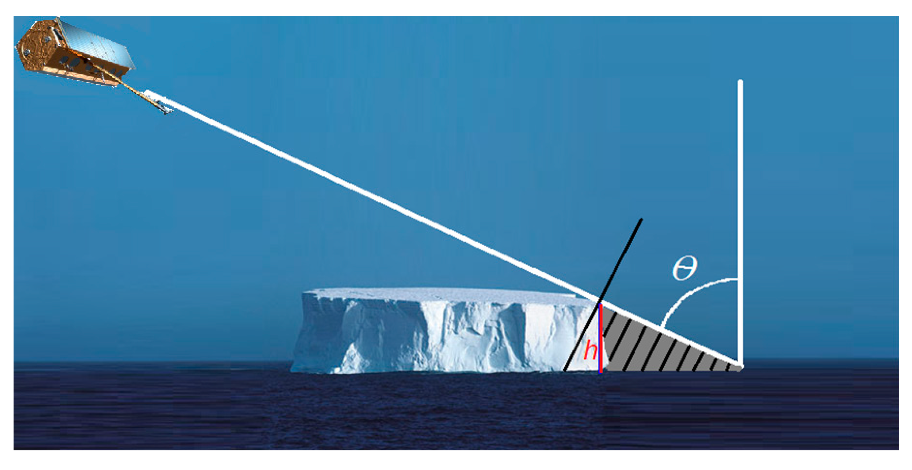
Discontinuous objects, such as icebergs, produce shadows in a SAR image (Figure 14). In this case, we can use shadows to determine the iceberg height from the shadow dimensions using Equation (3).
where s is length of the shadow in the slant range direction, and θ is the incidence angle.
h = s cos(θ)
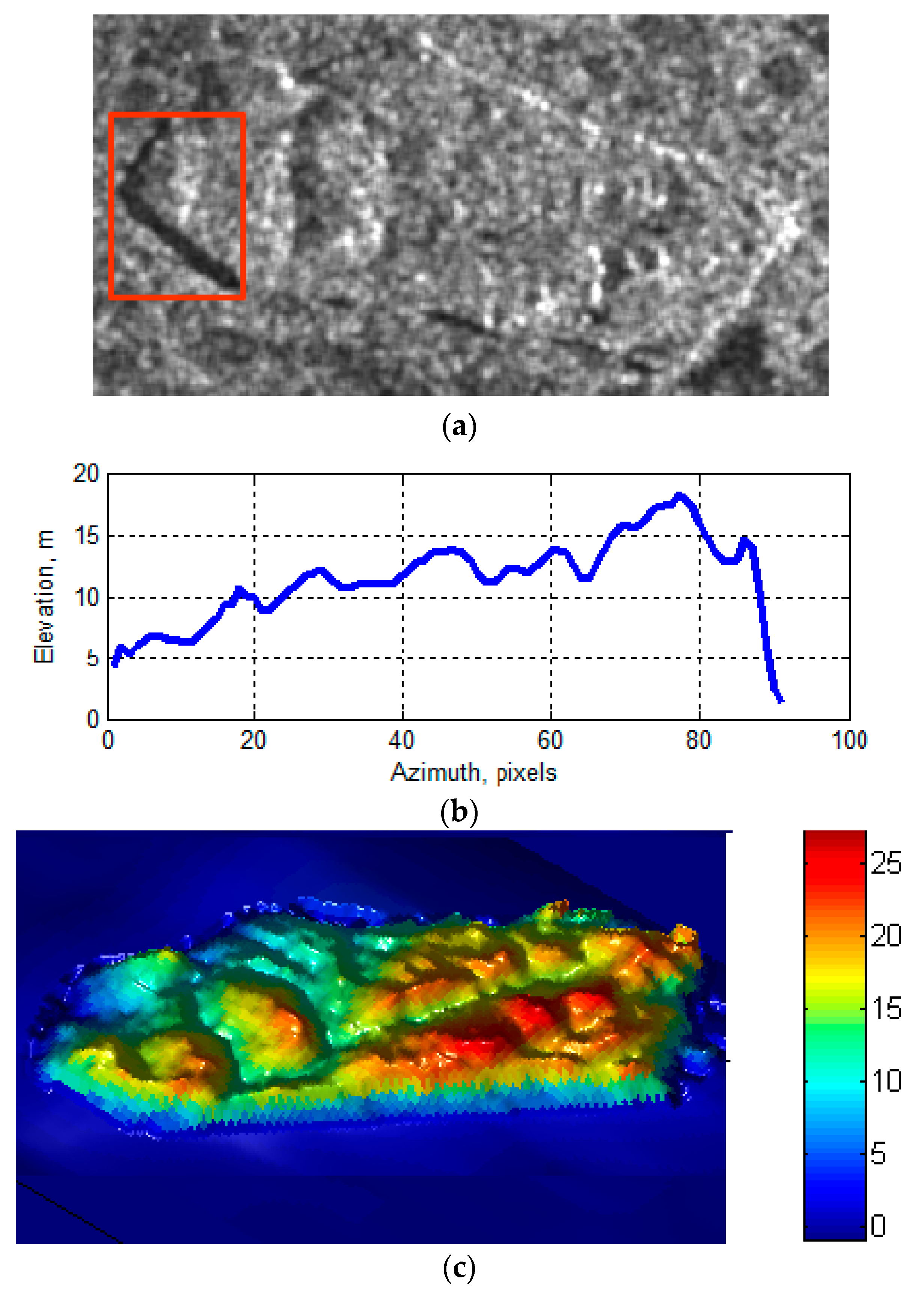
Figure 15 shows an iceberg shadow and the extracted elevation profile. The DEM generated using single-pass TDM InSAR can be used for verification of the extracted elevation. We can see that extracted elevation values range from 5 to 18 m, which corresponds to the InSAR DEM values.
3.2.4. Shape from Shading
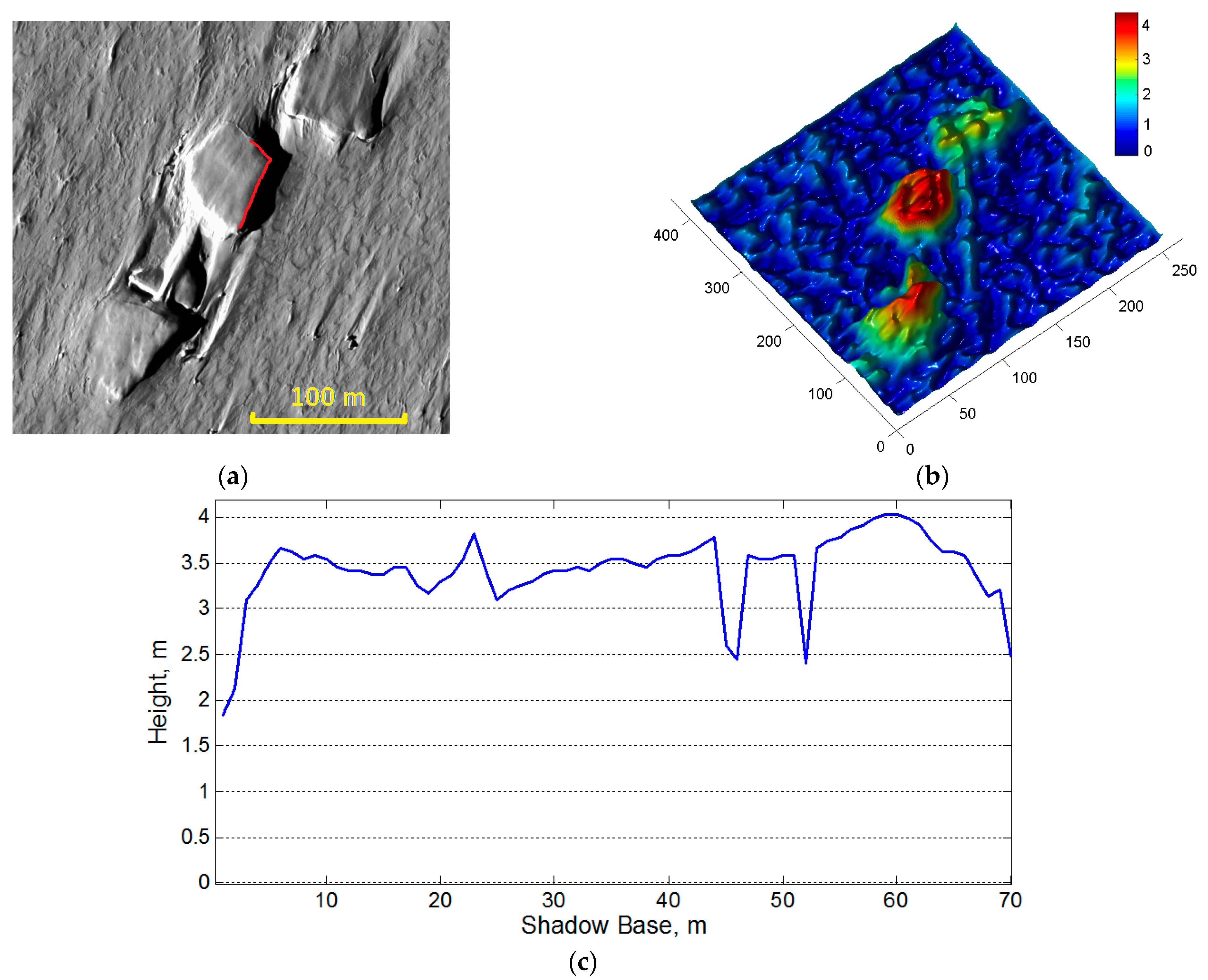
Iceberg surface topography can be extracted from the shape-from-shading technique [52,53]. In this technique, the relationship between the backscatter coefficient is linked to the local incidence angle (governed by the slope angle) used to reconstruct elevation information (topography) of a smooth surface based on its initial height. This method is feasible to measure topography from only one SAR intensity image, but it also requires information of coarse scale elevation. In our case, we used the freeboard estimated using the height-from-shadow technique described above.
This method considers that the SAR intensity is a function of the backscatter coefficient, resolution, incidence angle and slope. The ice backscattered coefficient is assumed to be constant, and it is known for X-band. Using an intensity image, we can estimate and consequently calculate an elevation increment (dH) for every resolution cell. The overall shape is calculated by integrating dH over the entire image. The results are strongly affected by speckle noise, and using speckle filtering is required to make this method robust.
The resulting DEM (Figure 16, top), generated using the shape-from-shading method applied to a single TerraSAR-X image, was compared with the interferometric TDM DEM (shown in Figure 15) by calculating the statistics of DEM differences (Figure 16, bottom). The comparison on a large iceberg (length greater than 120 m) demonstrated a good correlation between DEMs. The bias of DEM difference was 0.6 m, and the standard deviation was 2.7 m. It can be observed that the highest values of DEM difference (Figure 16, bottom) correspond to the edge of the iceberg, caused by a layover phenomenon.
3.2.5. Stereo-Radargrammetry
The stereo-radargrammetric method for DEM generation requires the collection of a stereo pair of images acquired from different incidence angles. Ultra-fine and fine-quad RS-2 images were acquired with different incidence angles to extract the DEMs of sea-ice and iceberg topography. Features common to both images are matched to estimate the stereo parallax, which can be used to calculate an elevation model of the area; therefore, this method is sensitive to dynamic environments such as sea ice. PCI Geomatica (CATALYST) Orthoengine was used to generate the DEMs of the RS-2 data of sea ice around areas near Meighen Island and in Baffin Bay with the technique described in [32].
Stereo pairs of images were tested in OrthoEngine, with varying parameters with or without applying speckle filters for separate test cases. Tests of stereo images show that a DEM of sea ice and large icebergs can be extracted; however, image matching quality is low for rubble fields, the smooth surfaces of multiyear (MY) ice and young level ice. Dynamic features, such as ice islands in Baffin Bay, can be displaced during the time difference for stereo data acquisition.
For the Baffin Bay data, RS-2 fine-quad FQ11 and FQ26 (Figure 17a,b) datasets were acquired with one day of time difference, and ice islands were not expected to move during that time period. After analyzing the DEMs extracted from the fine-quad data (Figure 17c), a number of icebergs could be found, which corresponded with the images.
4. Discussion
This study demonstrated the feasibility of existing satellite-based techniques for identifying and characterizing EIFs with a focus on hummocks and ice islands. The use of VHR electro-optical images enables identification of EIFs, relying on analyst experience. In addition, the VHR data can be applied to extract EIFs with the height-from-shadow technique. Height from shadow for ice ridge characterization is limited in the case when the ridge is aligned with the Sun’s illumination direction because, in this case, the shadow is broken into smaller patches and the ridge height cannot be accurately extracted.
The most accurate method for topography characterization and identification of EIFs is to apply the VHR electro-optical stereo DEM. This method demonstrated good agreement with other techniques including height from shadow. There are two main obstacles for wide application of VHR electro-optical data including stereo datasets for monitoring large Arctic areas: (i) high cost of imagery and (ii) small size of scene. With the current trends in the rapid development of new satellite constellations (e.g., Planet), the availability of VHR and high-resolution data is expected to improve in the future. In addition, the electro-optical and infrared imagery (VHR and medium resolution) are affected by visibility conditions because of the presence of clouds and fog, as well as the polar night phenomenon when the Sun remains below the horizon in winter months.
Medium-resolution Landsat-8 data are an important source of information for detection and identification of EIFs. As was demonstrated, the TIR band provides thermal contrast helpful to identify and detect thicker EIFs (hummocks and ice islands). The usage of the TIR band was limited for summer months when the ice surface warms up and starts melting. Also, TIR band resolution (120 m) is too coarse to observe small ice features. The main advantages of Landsat 8/9 are free data availability for all users, systematic coverage of the Canadian Arctic and the large image swath (185 km) allowing the monitoring of extended AOIs. Therefore, this data source is currently preferred in studying extreme ice features in the Canadian Arctic or the Arctic Ocean.
The single-pass InSAR technique using TDM data demonstrated excellent performance in the 3D mapping of hummocks and ice islands. The advantages of this technique are the all-weather and at-night capabilities that allow high confidence in operational data tasking. With an upcoming single-pass SAR mission such as Harmony, the usage of the InSAR method for sea-ice applications will become a commodity [54]. Potentially, this method can become operational for EIF monitoring.
The interesting results were achieved with the use of a single high-resolution SAR image for extracting height information from height from shadow and topography from shape using shading techniques. Results comparison with InSAR DEM demonstrated good performance. The main limitation of the shape-from-shading technique is the requirement of low or moderate topography of EIF. It is suitable for ice-island topography characterization but may not be so helpful for hummocks with high peaks. The high peaks problem can be addressed with the height-from-shadow method. These techniques, based on a single image, require VHR or high resolution, which are available with current and upcoming NewSpace constellations (e.g., ICEYE and Capella) and have the potential to become cost-efficient tools for EIF surveillance. However, both height from shadow and topography from shape using shading techniques require additional implementation for fully automated performance.
Full- and dual-polarimetric data are proven sources of information for sea-ice typing for many years. A volume-scattering component (HV) can be used to distinguish ice islands from sea ice, which has lower salinity and a lower volume component. The main limitation of full-polarimetric RS-2 data is its small image size compared to the ScanSAR images widely used for sea-ice monitoring. In addition, the polarimetric scattering mechanism may be influenced as temperature increases [12].
The new results on DEM extraction from an RS-2 stereo pair demonstrated the possibilities of the stereo radargrammetric technique for EIF applications. However, the stereo SAR data acquisition may require a substantial time difference in acquisition for a stereo pair (one day or more) and, therefore, will be limited for monitoring moving EIFs. In addition, the validation of stereo SAR results over sea ice require validation with more accurate data, such as VHR electro-optical stereo DEM.
5. Conclusions
The investigated techniques potentially can be used to detect and monitor EIFs in the Arctic. The proven methods can be based on single and/or stereo VHR electro-optical and infrared (EOIR) data, multispectral Landsat 8/9 imagery and VHR and high-resolution SAR data, including single-pass InSAR. The demonstrated single-image-based technique such as height from shadow can provide useful elevation information for EIF identification and characterization. These results are very important for multiple practical applications but especially in the offshore industry. Future work will be focused on automating these satellite-based techniques with machine learning, including deep learning algorithms. The data fusion of different bands can be investigated to improve detection confidence.
Author Contributions
Conceptualization, I.Z., P.B. and D.P.; methodology, I.Z.; software, I.Z. and M.H.; validation, I.Z. and M.H.; writing—original draft preparation, I.Z. and P.B.; writing—review and editing, I.Z., P.B. and D.P.; project administration, S.W.; funding acquisition, D.P. and P.B. All authors have read and agreed to the published version of the manuscript.
Funding
This research was funded by the Canadian Space Agency (CSA) under Earth Observation Application Development Program (EOADP) and LOOKNorth (C-CORE’s Center of Excellence).
Acknowledgments
The authors thank the German Aerospace Center (DLR) for the TerraSAR-X/TanDEM-X scientific data.
Conflicts of Interest
The authors declare no conflict of interest.
References
- Canadian Ice Service Manual of Ice (MANICE). Available online: https://www.canada.ca/en/environment-climate-change/services/weather-manuals-documentation/manice-manual-of-ice.html (accessed on 31 July 2023).
- Melling, H. Thickness of Multi-Year Sea Ice on the Northern Canadian Polar Shelf: A Second Look after 40 Years. Cryosphere 2022, 16, 3181–3197. [Google Scholar] [CrossRef]
- McGonigal, D.; Barrette, P.D. A Field Study of Grounded Ice Features and Associated Seabed Gouging in the Canadian Beaufort Sea. Cold Reg. Sci. Technol. 2018, 146, 142–154. [Google Scholar] [CrossRef]
- McGonigal, D.; Hagen, D.; Guzman, L. Extreme Ice Features Distribution in the Canadian Arctic. In Proceedings of the International Conference on Port and Ocean Engineering Under Arctic Conditions, Montreal, QC, Canada, 10–14 July 2011. [Google Scholar]
- Pilkington, G.; Hill, M.; Metge, M.; McGonigal, D. Beaufort Sea Ice Design Criteria: Acquisition of Data on EIFs [Extreme Ice Features]; Canatec Consultants Ltd.: Calgary, AB, Canada, 1992; p. 154. [Google Scholar]
- Barber, D.G.; McCullough, G.; Babb, D.; Komarov, A.S.; Candlish, L.M.; Lukovich, J.V.; Asplin, M.; Prinsenberg, S.; Dmitrenko, I.; Rysgaard, S. Climate Change and Ice Hazards in the Beaufort Sea. Elem. Sci. Anthr. 2014, 2, 25. [Google Scholar] [CrossRef]
- Galley, R.J.; Else, B.G.T.; Prinsenberg, S.J.; Babb, D.; Barber, D.G. Summer Sea Ice Concentration, Motion, and Thickness Near Areas of Proposed Offshore Oil and Gas Development in the Canadian Beaufort Sea—2009. Arctic 2013, 66, 105–116. [Google Scholar] [CrossRef]
- Bowditch, N. American Practical Navigator, An Epitome of Navigation; Pub. No. 9; National Imaging and Mapping Agency: Bethesda, Maryland, 2002. [Google Scholar]
- Barker, A.; De Abreu, R.; Timco, G.W. Satellite Detection and Monitoring of Sea Ice Rubble Fields. In Proceedings of the 19th IAHR Symposium on Ice, Vancouver, BC, Canada, 6–11 July 2008; Volume 1, pp. 419–430. [Google Scholar]
- Dierking, W.; Dall, J. Sea-Ice Deformation State from Synthetic Aperture Radar Imagery—Part I: Comparison of C-and L-Band and Different Polarization. Geosci. Remote Sens. IEEE Trans. 2007, 45, 3610–3622. [Google Scholar] [CrossRef]
- Zhang, Y.; Touzi, R.; Feng, W.; Hong, G.; Lantz, T.C.; Kokelj, S.V. Landscape-scale Variations in Near-surface Soil Temperature and Active-layer Thickness: Implications for High-resolution Permafrost Mapping. Permafr. Periglac. Process 2021, 32, 627–640. [Google Scholar] [CrossRef]
- Park, S.-E. Variations of Microwave Scattering Properties by Seasonal Freeze/Thaw Transition in the Permafrost Active Layer Observed by ALOS PALSAR Polarimetric Data. Remote Sens. 2015, 7, 17135–17148. [Google Scholar] [CrossRef]
- Usami, N.; Muhuri, A.; Bhattacharya, A.; Hirose, A. Proposal of Wet Snowmapping with Focus on Incident Angle Influential to Depolarization of Surface Scattering. In Proceedings of the 2016 IEEE International Geoscience and Remote Sensing Symposium (IGARSS), Beijing, China, 10–15 July 2016; pp. 1544–1547. [Google Scholar]
- Tsai, Y.-L.S.; Dietz, A.; Oppelt, N.; Kuenzer, C. Remote Sensing of Snow Cover Using Spaceborne SAR: A Review. Remote Sens. 2019, 11, 1456. [Google Scholar] [CrossRef]
- Canatec. Beaufort and Chukchi Seas Design Criteria—Extreme Ice Features and Multi-Year Floe/Ridge Statistics; Canatec Associates International Ltd.: Calgary, AB, Canada, 2010. [Google Scholar]
- Gill, J.; Yackel, J. Evaluation of C-Band SAR Polarimetric Parameters for Discrimination of First-Year Sea Ice Types. Can. J. Remote Sens. 2012, 38, 306–323. [Google Scholar] [CrossRef]
- Zakharov, I.; Bobby, P.; Power, D.; Warren, S. Monitoring Extreme Ice Features Using Multi-Resolution RADARSAT-2 Data. In Proceedings of the Geoscience and Remote Sensing Symposium (IGARSS), 2014 IEEE International, Quebec City, QC, Canada, 13–18 July 2014; pp. 3972–3975. [Google Scholar]
- Leira, B.J.; Chai, W.; Radhakrishnan, G. On Characteristics of Ice Ridges and Icebergs for Design of Ship Hulls in Polar Regions Based on Environmental Design Contours. Appl. Sci. 2021, 11, 5749. [Google Scholar] [CrossRef]
- Mussells, O.; Dawson, J.; Howell, S. Using RADARSAT to Identify Sea Ice Ridges and Their Implications for Shipping in Canada’s Hudson Strait. Arctic 2016, 69, 421–433. [Google Scholar] [CrossRef]
- Duncan, K.; Farrell, S.L. Determining Variability in Arctic Sea Ice Pressure Ridge Topography with ICESat-2. Geophys. Res. Lett. 2022, 49, e2022GL100272. [Google Scholar] [CrossRef]
- Lensu, M.; Similä, M. Ice Ridge Density Signatures in High-Resolution SAR Images. Cryosphere 2022, 16, 4363–4377. [Google Scholar] [CrossRef]
- Power, D.; Youden, J.; Lane, K.; Randell, C.; Flett, D. Iceberg Detection Capabilities of RADARSAT Synthetic Aperture Radar. Can. J. Remote Sens. 2001, 27, 476–486. [Google Scholar] [CrossRef]
- Karvonen, J.; Gegiuc, A.; Niskanen, T.; Montonen, A.; Buus-Hinkler, J.; Rinne, E. Iceberg Detection in Dual-Polarized C-Band SAR Imagery by Segmentation and Nonparametric CFAR (SnP-CFAR). IEEE Trans. Geosci. Remote Sens. 2022, 60, 4300812. [Google Scholar] [CrossRef]
- Haas, C. Airborne Observations of the Distribution, Thickness, and Drift of Different Sea Ice Types and Extreme Ice Features in the Canadian Beaufort Sea. In The All Days; Paper Number OTC-23812; OTC: Houston, TX, USA, 2012. [Google Scholar]
- Dawson, G.; Landy, J.; Tsamados, M.; Komarov, A.S.; Howell, S.; Heorton, H.; Krumpen, T. A 10-Year Record of Arctic Summer Sea Ice Freeboard from CryoSat-2. Remote Sens. Environ. 2022, 268, 112744. [Google Scholar] [CrossRef]
- Tournadre, J.; Bouhier, N.; Girard-Ardhuin, F.; Rémy, F. Large Icebergs Characteristics from Altimeter Waveforms Analysis. J. Geophys. Res. Ocean. 2015, 120, 1954–1974. [Google Scholar] [CrossRef]
- Zakharov, I.; Bobby, P.; Power, D.; Warren, S.; Howell, M. Detection and Characterization of Extreme Ice Features in Single High Resolution Satellite Imagery. In Proceedings of the 2014 IEEE Geoscience and Remote Sensing Symposium, Quebec City, QC, Canada, 13–18 July 2014; pp. 3965–3968. [Google Scholar]
- Dierking, W.; Lang, O.; Busche, T. Sea Ice Local Surface Topography from Single-Pass Satellite InSAR Measurements: A Feasibility Study. Cryosphere 2017, 11, 1967–1985. [Google Scholar] [CrossRef]
- Dammann, D.O.; Eriksson, L.E.B.; Nghiem, S.V.; Pettit, E.C.; Kurtz, N.T.; Sonntag, J.G.; Busche, T.E.; Meyer, F.J.; Mahoney, A.R. Iceberg Topography and Volume Classification Using TanDEM-X Interferometry. Cryosphere 2019, 13, 1861–1875. [Google Scholar] [CrossRef]
- Zakharov, I.; Puestow, T.; Power, D.; Howell, M. Icebergs in Sea Ice with TanDEM-X Interferometry. IEEE Geosci. Remote Sens. Lett. 2019, 16, 1070–1074. [Google Scholar] [CrossRef]
- Toutin, T.; Schmitt, C.; Berthier, E.; Clavet, D. DEM Generation over Ice Fields in the Canadian Arctic with Along-Track SPOT5 HRS Stereo Data. Can. J. Remote Sens. 2011, 37, 429–438. [Google Scholar] [CrossRef]
- Zakharov, I.; Toutin, T. StereoPol Radarsat-2 Data Fusion in Radargrammetry. Can. J. Remote Sens. 2011, 37, 452–463. [Google Scholar] [CrossRef]
- Gruber, A.; Wessel, B.; Huber, M.; Roth, A. Operational TanDEM-X DEM Calibration and First Validation Results. ISPRS J. Photogramm. Remote Sens. 2012, 73, 39–49. [Google Scholar] [CrossRef]
- Sefercik, U.G.; Buyuksalih, G.; Atalay, C. DSM Generation with Bistatic TanDEM-X InSAR Pairs and Quality Validation in Inclined Topographies and Various Land Cover Classes. Arab. J. Geosci. 2020, 13, 560. [Google Scholar] [CrossRef]
- Huber, M.; Gruber, A.; Wendleder, A.; Wessel, B.; Roth, A.; Schmitt, A. The global tandem-x dem: Production status and first validation results. Int. Arch. Photogramm. Remote Sens. Spat. Inf. Sci. 2012, 39, 45–50. [Google Scholar] [CrossRef]
- Redlin, L.; Viet, N.; Watson, S. Thales’ Shadow. Math. Mag. 2000, 73, 347–353. [Google Scholar] [CrossRef]
- Kwok, R. Declassified High-Resolution Visible Imagery for Arctic Sea Ice Investigations: An Overview. Remote Sens. Environ. 2014, 142, 44–56. [Google Scholar] [CrossRef]
- Xie, Y.; Feng, D.; Xiong, S.; Zhu, J.; Liu, Y. Multi-Scene Building Height Estimation Method Based on Shadow in High Resolution Imagery. Remote Sens. 2021, 13, 2862. [Google Scholar] [CrossRef]
- Bennett, A.J.; Blacknell, D. The Extraction of Building Dimensions from High Resolution SAR Imagery. In Proceedings of the 2003 Proceedings of the International Conference on Radar (IEEE Cat. No.03EX695), Adelaide, SA, Australia, 3–5 September 2003; pp. 182–187. [Google Scholar]
- Brunner, D.; Lemoine, G.; Bruzzone, L.; Greidanus, H. Building Height Retrieval From VHR SAR Imagery Based on an Iterative Simulation and Matching Technique. IEEE Trans. Geosci. Remote Sens. 2010, 48, 1487–1504. [Google Scholar] [CrossRef]
- Guida, R.; Iodice, A.; Riccio, D. Height Retrieval of Isolated Buildings From Single High-Resolution SAR Images. IEEE Trans. Geosci. Remote Sens. 2010, 48, 2967–2979. [Google Scholar] [CrossRef]
- Sportouche, H.; Tupin, F.; Denise, L. Extraction and Three-Dimensional Reconstruction of Isolated Buildings in Urban Scenes From High-Resolution Optical and SAR Spaceborne Images. IEEE Trans. Geosci. Remote Sens. 2011, 49, 3932–3946. [Google Scholar] [CrossRef]
- Sun, Y.; Mou, L.; Wang, Y.; Montazeri, S.; Zhu, X.X. Large-Scale Building Height Retrieval from Single SAR Imagery Based on Bounding Box Regression Networks. ISPRS J. Photogramm. Remote Sens. 2022, 184, 79–95. [Google Scholar] [CrossRef]
- Christensen, E.; Luzader, J. From Sea to Air to Space: A Century of Iceberg Tracking Technology. Coast Guard. J. Saf. Secur. Sea Proc. Mar. Saf. Secur. Counc. 2012, 69, 17–22. [Google Scholar]
- Johannessen, O.; Alexandrov, V.; Frolov, I.Y.; Sandven, S.; Pettersson, L.; Bobylev, L.P.; Kloster, K.; Smirnov, V.; Mironov, Y.; Babich, N. Remote Sensing of Sea Ice in the Northern Sea Route: Studies and Applications; Springer Science & Business Media: New York, NY, USA, 2006. [Google Scholar]
- Hyun, C.-U.; Kim, J.-H.; Han, H.; Kim, H. Mosaicking Opportunistically Acquired Very High-Resolution Helicopter-Borne Images over Drifting Sea Ice Using COTS Sensors. Sensors 2019, 19, 1251. [Google Scholar] [CrossRef] [PubMed]
- Jeffries, M.O. Arctic Ice Shelves and Ice Islands: Origin, Growth and Disintegration, Physical Characteristics, Structural-Stratigraphic Variability, and Dynamics. Rev. Geophys. 1992, 30, 245. [Google Scholar] [CrossRef]
- Rajji, A.; Najine, A.; WAFIK, A.; Benmoussa, A. Building Height Estimation from High Resolution Satellite Images. Int. J. Innov. Appl. Stud. 2022, 35, 268–281. [Google Scholar]
- Lytle, V.I.; Worby, A.; Massom, R. Sea-Ice Pressure Ridges in East Antarctica. Ann. Glaciol. 1998, 27, 449–454. [Google Scholar] [CrossRef]
- Huang, X.; Keong, L. Kwoh 3D Building Reconstruction and Visualization for Single High Resolution Satellite Image. In Proceedings of the 2007 IEEE International Geoscience and Remote Sensing Symposium, Barcelona, Spain, 23–28 July 2007; pp. 5009–5012. [Google Scholar]
- Lee, J.-S.; Pottier, E. Polarimetric Radar Imaging: From Basics to Applications; CRC Press: Boca Raton, FL, USA, 2009. [Google Scholar]
- Frankot, R.T.; Chellappa, R. Estimation of Surface Topography from SAR Imagery Using Shape from Shading Techniques. Artif. Intell. 1990, 43, 271–310. [Google Scholar] [CrossRef]
- Hurt, N.E. Mathematical Methods in Shape-from-Shading: A Review of Recent Results. Acta Appl. Math. 1991, 23, 163–188. [Google Scholar] [CrossRef]
- Kleinherenbrink, M.; Korosov, A.; Newman, T.; Theodosiou, A.; Li, Y.; Mulder, G.; Rampal, P.; Stroeve, J.; Lopez-Dekker, P. Estimating Instantaneous Sea-Ice Dynamics from Space Using Thebi-Static Radar Measurements of Earth Explorer 10 Candidate Harmony. Cryosphere 2021, 15, 3101–3118. [Google Scholar] [CrossRef]
Figure 1.
Map of Study Areas.
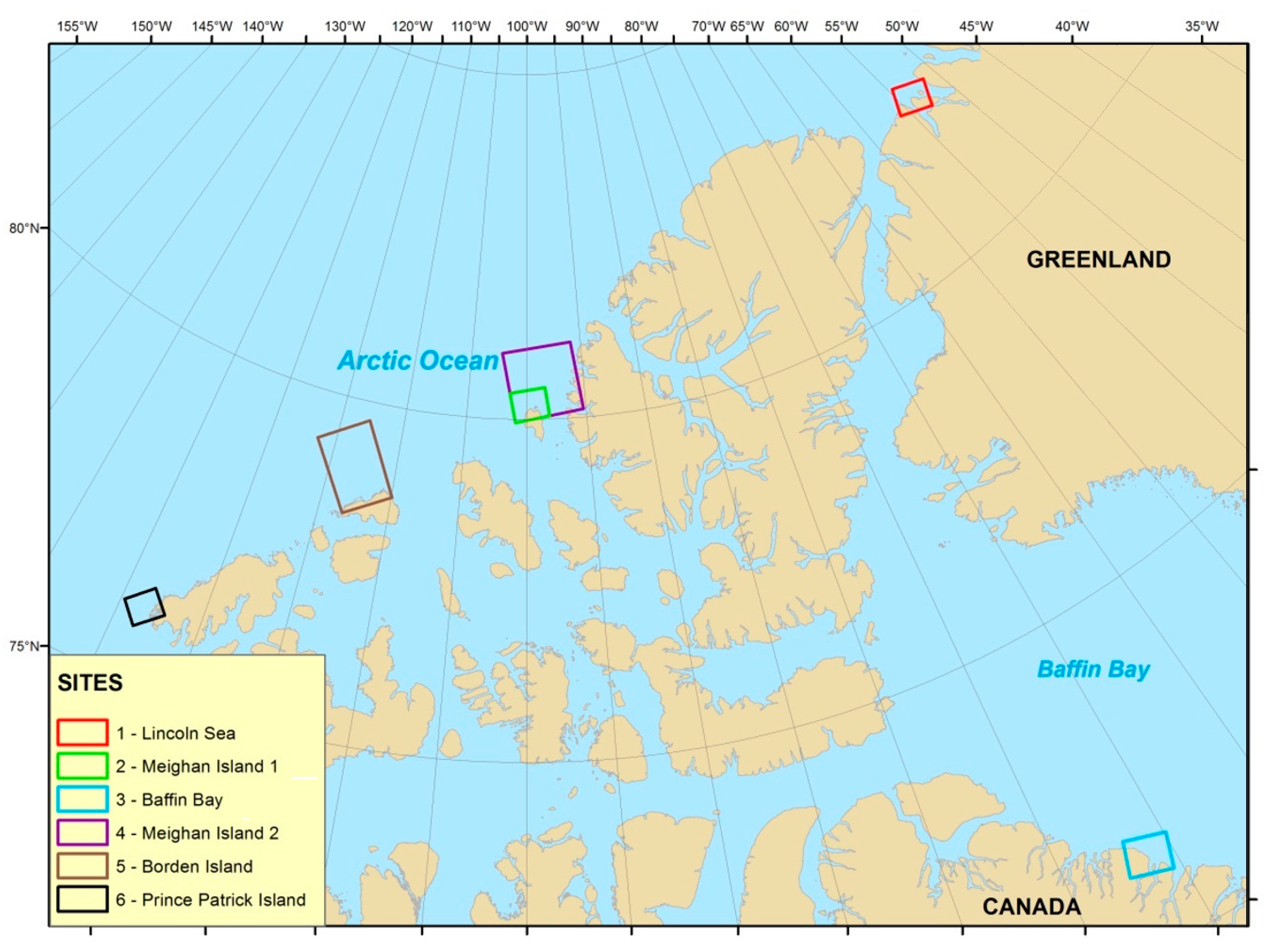
Figure 2.
Ice island (a) and ice-island fragments (b) in WorldView-2 image. Images © DigitalGlobe, 2014.
Figure 2.
Ice island (a) and ice-island fragments (b) in WorldView-2 image. Images © DigitalGlobe, 2014.
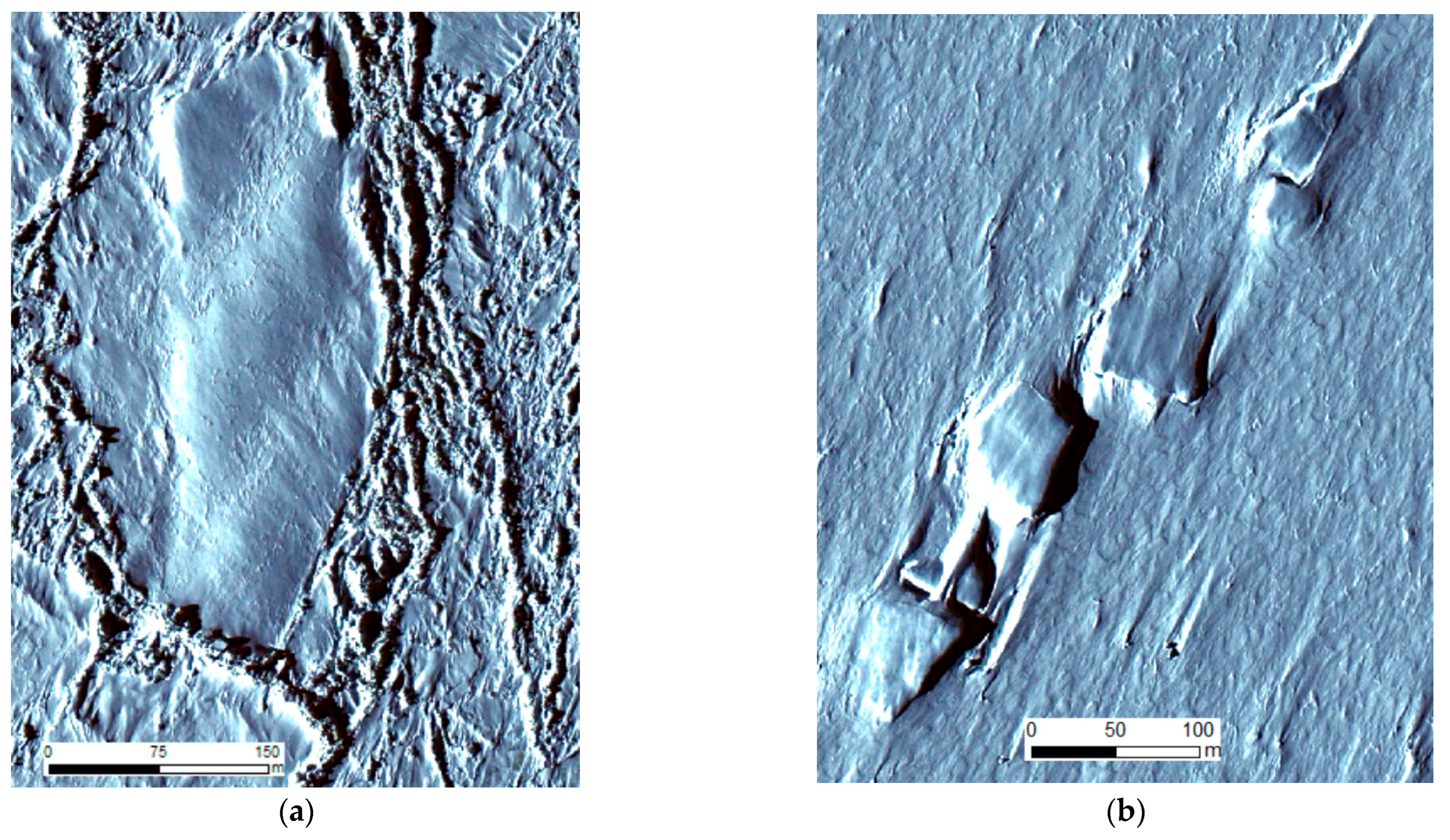
Figure 3.
A fragment of one of stereo SPOT 6 imagery (a) over Axel Heiberg Island used to generate DEM (b) over the corresponded area. SPOT 6 image © Airbus Defence and Space 2014.
Figure 3.
A fragment of one of stereo SPOT 6 imagery (a) over Axel Heiberg Island used to generate DEM (b) over the corresponded area. SPOT 6 image © Airbus Defence and Space 2014.

Figure 4.
MYHF on a WorldView-2 image (a) and DEM (b); rubble field shown in WorldView-2 image (c) and in DEM (d). Images © DigitalGlobe, 2014.
Figure 4.
MYHF on a WorldView-2 image (a) and DEM (b); rubble field shown in WorldView-2 image (c) and in DEM (d). Images © DigitalGlobe, 2014.

Figure 5.
Acquisition geometry for image of the ridge: (a) the azimuth and the elevation angles for the sun and the satellite, (b) explanatory diagram of the ridge and shadow.
Figure 5.
Acquisition geometry for image of the ridge: (a) the azimuth and the elevation angles for the sun and the satellite, (b) explanatory diagram of the ridge and shadow.
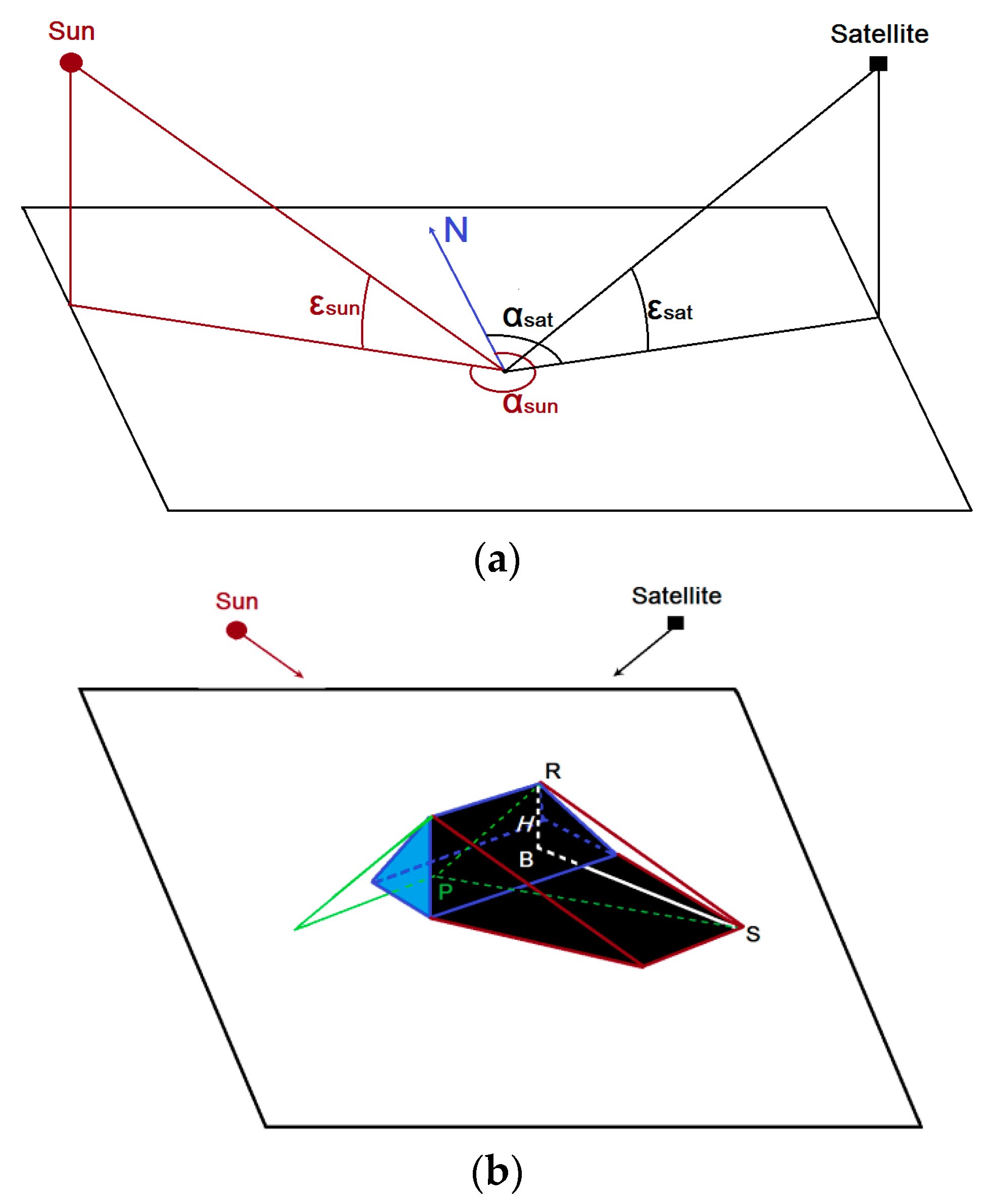
Figure 6.
WorldView-2 image with ice-island fragments with red line indicating edge used for height estimation (a); stereo DEM of these ice-island fragments (b); and height profile extracted using Equation (2) along the shadow base (c). Images © DigitalGlobe, 2014.
Figure 6.
WorldView-2 image with ice-island fragments with red line indicating edge used for height estimation (a); stereo DEM of these ice-island fragments (b); and height profile extracted using Equation (2) along the shadow base (c). Images © DigitalGlobe, 2014.

Figure 7.
WorldView-2 images of ice features used to estimate height from shadow. Images © DigitalGlobe, 2014. (a)—ice island, (c)—forming hummock, (b,d)—ice island fragments.
Figure 7.
WorldView-2 images of ice features used to estimate height from shadow. Images © DigitalGlobe, 2014. (a)—ice island, (c)—forming hummock, (b,d)—ice island fragments.

Figure 8.
Monitoring the hummock-forming process with pansharpened Landsat 8 images. Landsat 8 images courtesy of the U.S. Geological Survey.
Figure 8.
Monitoring the hummock-forming process with pansharpened Landsat 8 images. Landsat 8 images courtesy of the U.S. Geological Survey.

Figure 9.
Ice island: (a) WorldView-2 image; (b) perspective view of Stereo DEM; (c) Landsat 8 pansharpened RGB bands; (d) Landsat 8 thermal infrared band, shown as dark areas. WorldView-2 Images © DigitalGlobe, 2014. Landsat 8 images courtesy of the U.S. Geological Survey.
Figure 9.
Ice island: (a) WorldView-2 image; (b) perspective view of Stereo DEM; (c) Landsat 8 pansharpened RGB bands; (d) Landsat 8 thermal infrared band, shown as dark areas. WorldView-2 Images © DigitalGlobe, 2014. Landsat 8 images courtesy of the U.S. Geological Survey.

Figure 10.
Multiyear hummock fields: (a) WorldView-2 image; (b) perspective view of Stereo DEM; (c) Landsat 8 pansharpened RGB bands; (d) Landsat 8 thermal infrared band. WorldView-2 images © DigitalGlobe, 2014. Landsat 8 images courtesy of the U.S. Geological Survey.
Figure 10.
Multiyear hummock fields: (a) WorldView-2 image; (b) perspective view of Stereo DEM; (c) Landsat 8 pansharpened RGB bands; (d) Landsat 8 thermal infrared band. WorldView-2 images © DigitalGlobe, 2014. Landsat 8 images courtesy of the U.S. Geological Survey.

Figure 11.
Single-pass TDM InSAR DEM over hummock (a); WorldView-2 image (b) and stereo DEM over the same area (c). WorldView-2 images © DigitalGlobe, 2014.
Figure 11.
Single-pass TDM InSAR DEM over hummock (a); WorldView-2 image (b) and stereo DEM over the same area (c). WorldView-2 images © DigitalGlobe, 2014.
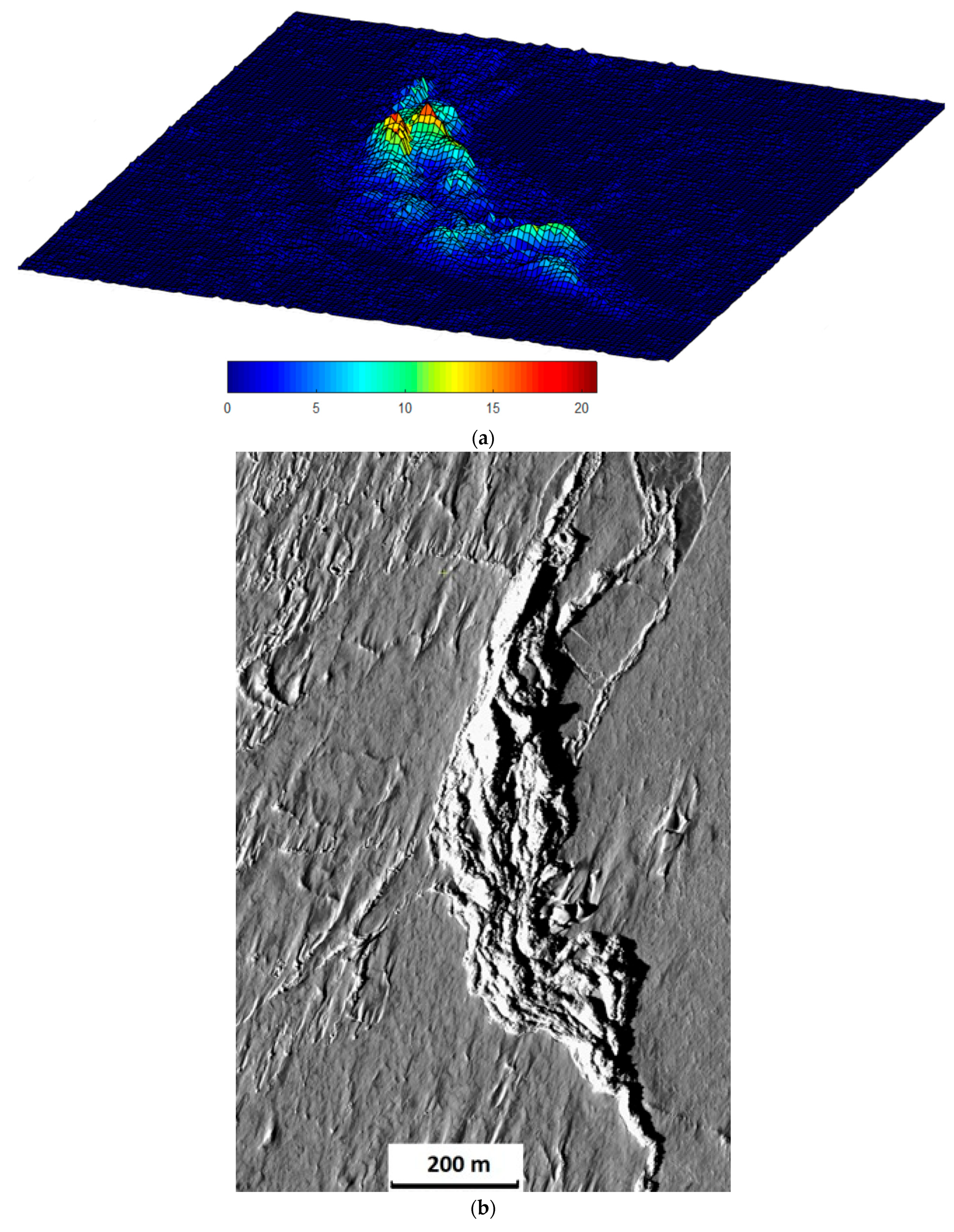
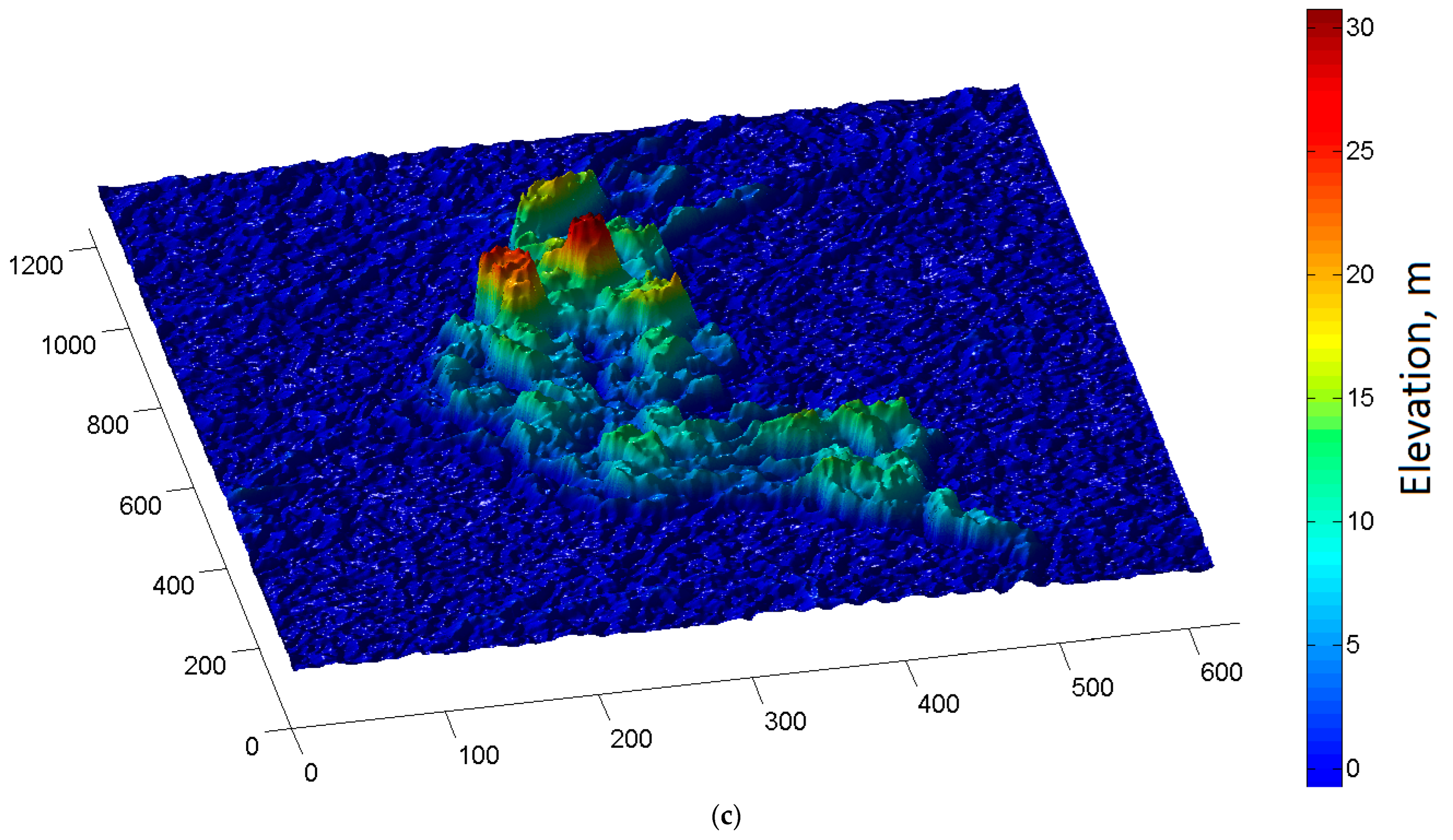
Figure 12.
Icebergs in sea ice shown in GeoEye-1 image, acquired on 22 September 2014 (top) and in RS-2 RGB image of Pauli decomposition ( blue, red and green) of FQ mode (26 September 2013) (middle) and FQW (7 March 2014) (bottom). GeoEye-1 satellite image courtesy of GeoEye-1 © DigitalGlobe (presently it is MAXAR Technologies). RADARSAT-2 Data and Products © MDA Ltd. (2013)—All Rights Reserved.
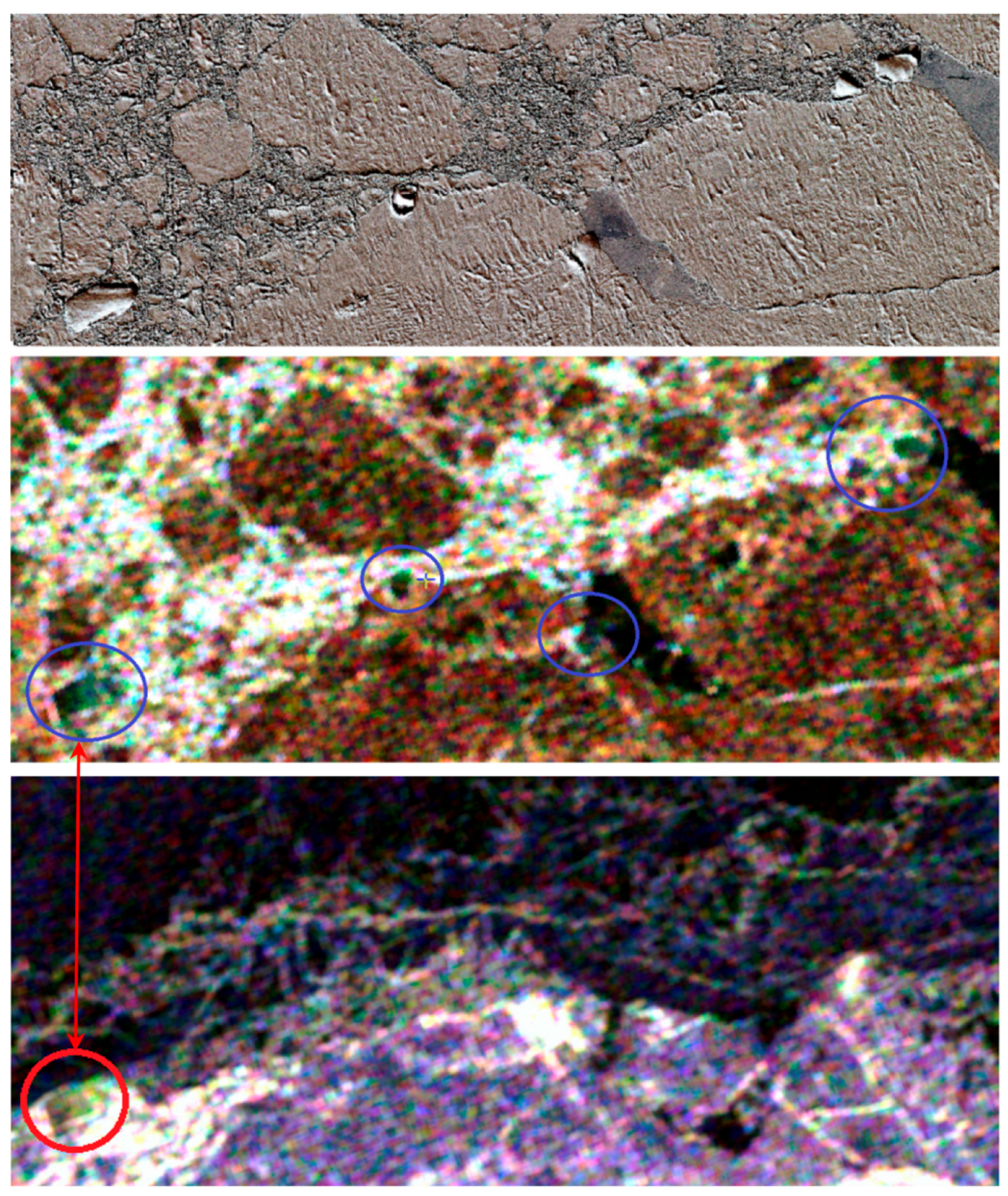
Figure 13.
Color composites of dual-polarized RS-2 imagery of standard beam mode S8 acquired on 3 March 2014: HH (a), HV (b), RGB color composite image (HH—red, HV—green, HH—blue) (c), and Landsat 8 image (d); (e) is the enlarged color composite, and (f) is Landsat 8 of ice island. Landsat 8 images courtesy of the U.S. Geological Survey. RADARSAT-2 data and products © MDA Ltd. (2014)—all rights reserved.

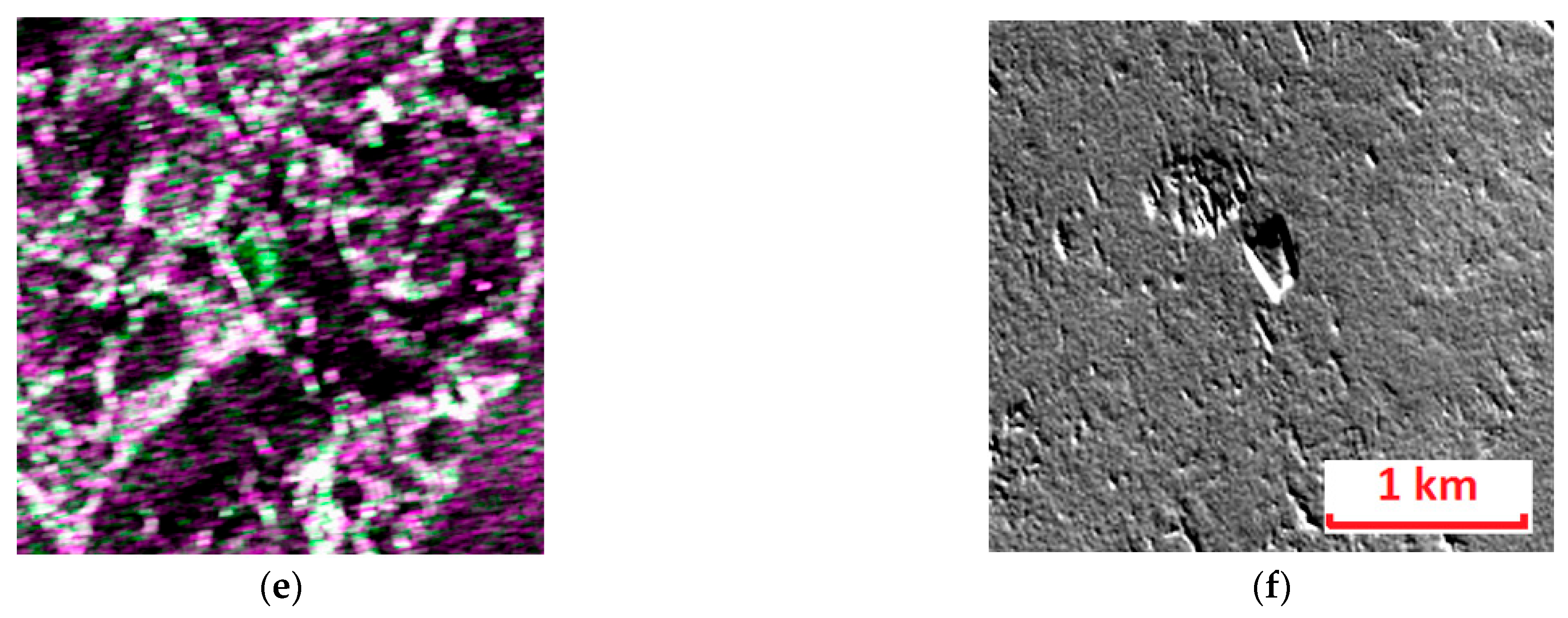
Figure 14.
Geometry of SAR data acquisition (θ—incidence angle) over ice island with freeboard (h).

Figure 15.
Shadow of iceberg highlighted in red rectangle in TerraSAR-X image (a); extracted elevation profile using Equation (3) (b); DEM generated using single-pass TDM InSAR pair (c). TerraSAR-X/TanDEM-X data © DLR.
Figure 15.
Shadow of iceberg highlighted in red rectangle in TerraSAR-X image (a); extracted elevation profile using Equation (3) (b); DEM generated using single-pass TDM InSAR pair (c). TerraSAR-X/TanDEM-X data © DLR.

Figure 16.
Ice-island topography extracted using shape-from-shading technique (a); difference of DEMs (in m) generated using a single-pass TDM InSAR pair (b).
Figure 16.
Ice-island topography extracted using shape-from-shading technique (a); difference of DEMs (in m) generated using a single-pass TDM InSAR pair (b).
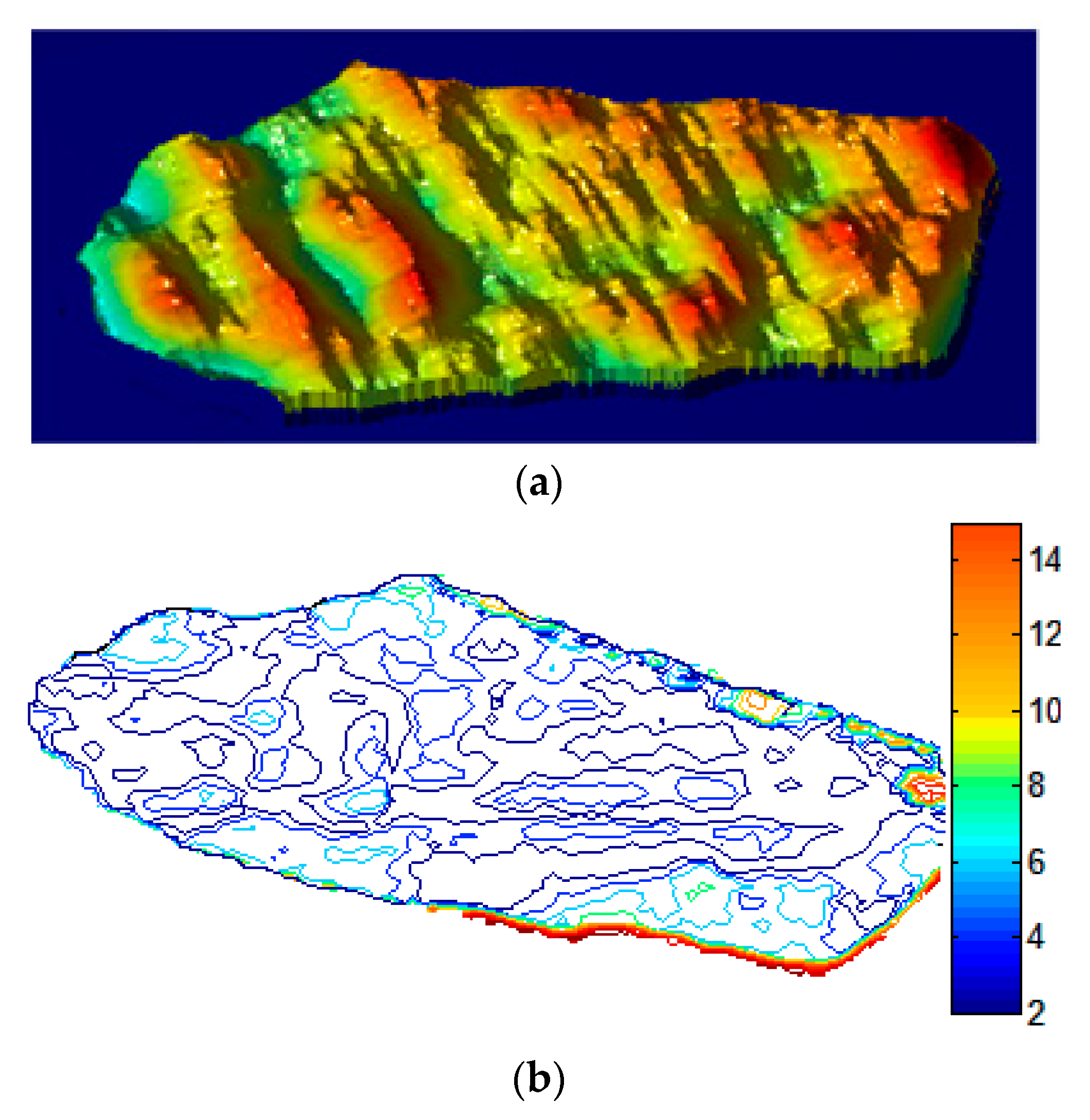
Figure 17.
Fine-quad data (FQ11 on (a)) and (FQ26 on (b)) represented as color composite R (HH)-G (HV)-B(VV) (a,b); DEM extracted over area shown in the previous figure (c). RADARSAT-2 data and products © MDA Ltd. (2013)—all rights reserved.
Figure 17.
Fine-quad data (FQ11 on (a)) and (FQ26 on (b)) represented as color composite R (HH)-G (HV)-B(VV) (a,b); DEM extracted over area shown in the previous figure (c). RADARSAT-2 data and products © MDA Ltd. (2013)—all rights reserved.

Disclaimer/Publisher’s Note: The statements, opinions and data contained in all publications are solely those of the individual author(s) and contributor(s) and not of MDPI and/or the editor(s). MDPI and/or the editor(s) disclaim responsibility for any injury to people or property resulting from any ideas, methods, instructions or products referred to in the content. |
© 2023 by the authors. Licensee MDPI, Basel, Switzerland. This article is an open access article distributed under the terms and conditions of the Creative Commons Attribution (CC BY) license (https://creativecommons.org/licenses/by/4.0/).
Share and Cite
MDPI and ACS Style
Zakharov, I.; Bobby, P.; Power, D.; Warren, S.; Howell, M. Satellite-Based Identification and Characterization of Extreme Ice Features: Hummocks and Ice Islands. Remote Sens. 2023, 15, 4065. https://doi.org/10.3390/rs15164065
AMA Style
Zakharov I, Bobby P, Power D, Warren S, Howell M. Satellite-Based Identification and Characterization of Extreme Ice Features: Hummocks and Ice Islands. Remote Sensing. 2023; 15(16):4065. https://doi.org/10.3390/rs15164065
Chicago/Turabian StyleZakharov, Igor, Pradeep Bobby, Desmond Power, Sherry Warren, and Mark Howell. 2023. "Satellite-Based Identification and Characterization of Extreme Ice Features: Hummocks and Ice Islands" Remote Sensing 15, no. 16: 4065. https://doi.org/10.3390/rs15164065
Note that from the first issue of 2016, this journal uses article numbers instead of page numbers. See further details here.