

Imitation Learning through Image Augmentation Using Enhanced Swin Transformer Model in Remote Sensing

1
Department of Autonomous Things Intelligence Graduate School, Dongguk University-Seoul, Seoul 04620, Republic of Korea
2
Division of AI Software Convergence, Dongguk University-Seoul, Seoul 04620, Republic of Korea
*
Author to whom correspondence should be addressed.
Remote Sens. 2023, 15(17), 4147; https://doi.org/10.3390/rs15174147
Submission received: 6 July 2023
/
Revised: 11 August 2023
/
Accepted: 21 August 2023
/
Published: 24 August 2023
(This article belongs to the Special Issue Advances in Deep Learning Approaches in Remote Sensing)
Abstract
:In unmanned systems, remote sensing is an approach that collects and analyzes data such as visual images, infrared thermal images, and LiDAR sensor data from a distance using a system that operates without human intervention. Recent advancements in deep learning enable the direct mapping of input images in remote sensing to desired outputs, making it possible to learn through imitation learning and for unmanned systems to learn by collecting and analyzing those images. In the case of autonomous cars, raw high-dimensional data are collected using sensors, which are mapped to the values of steering and throttle through a deep learning network to train imitation learning. Therefore, by imitation learning, the unmanned systems observe expert demonstrations and learn expert policies, even in complex environments. However, in imitation learning, collecting and analyzing a large number of images from the game environment incurs time and costs. Training with a limited dataset leads to a lack of understanding of the environment. There are some augmentation approaches that have the limitation of increasing the dataset because of considering only the locations of objects visited and estimated. Therefore, it is required to consider the diverse kinds of the location of objects not visited to solve the limitation. This paper proposes an enhanced model to augment the number of training images comprising a Preprocessor, an enhanced Swin Transformer model, and an Action model. Using the original network structure of the Swin Transformer model for image augmentation in imitation learning is challenging. Therefore, the internal structure of the Swin Transformer model is enhanced, and the Preprocessor and Action model are combined to augment training images. The proposed method was verified through an experimental process by learning from expert demonstrations and augmented images, which reduced the total loss from 1.24068 to 0.41616. Compared to expert demonstrations, the accuracy was approximately 86.4%, and the proposed method achieved 920 points and 1200 points more than the comparison model to verify generalization.
1. Introduction
Recently, with the development of deep learning [1,2,3], imitation learning has been applied in various unmanned system-related domains, such as robotics [4,5] and autonomous vehicles [6,7]. The combination of imitation learning and remote sensing leads to advanced controls based on real-time analysis of incoming sensor data. By learning the historical controls of an expert, the unmanned systems learn to navigate autonomously and adjust their controls based on environmental conditions. For instance, unmanned aerial vehicles (UAVs) equipped with image sensors can learn to mimic the flight patterns of experienced human operators using raw omnidirectional images as inputs, predicting flight commands that match the commands of the expert. Therefore, imitation learning is an approach where an agent learns to perform tasks by mimicking the control patterns of an expert. They are categorized as inverse reinforcement learning (IRL) and behavioral cloning (BC). IRL [8] is an algorithm that infers a reward function based on an agent’s observed actions. This is useful when it is difficult to define a reward function manually in a complex environment. However, IRL requires a large amount of training data, and identifying the correct reward function is computationally expensive, which makes it challenging for practical use. In contrast, the basic idea behind BC [9] is to learn a policy that maps states to actions by observing the actions of experts in similar states. Learning from examples of expert demonstrations reduces the training time and computational resources needed to achieve high performance because the agent does not have to rely on trial and error. However, learning using a limited dataset may only perform well if the state space is included in the expert dataset [10]. Therefore, obtaining datasets of various states for practical applications is important.
Data augmentation is used to generate additional training data that capture various images. Data augmentation is commonly used in behavior cloning and can be applied to various image types, which generates new training images by applying various transformations to collected images. Transformations include geometric transformations such as flipping, rotation, and cropping [11], random erasing [12], photometric transformations such as color space transformations [13] and deep learning-based approaches such as adversarial training [14], neural style transfer [15], and GAN [16]-based data augmentation [17]. The model enables learning various images from limited training images by introducing variations to collected images. However, data augmentation approaches do not augment images considering objects within the images. Understanding the arrangements of objects in the images helps the model outperform the model trained with a typical global representation of images.
Research has explored image augmentation by considering objects within images. Examples include augmentation approaches based on the contour of an object considering the shape of the object [18] or scene composition augmentation that replaces some objects in the data with other objects [19]. In imitation learning, the learning arrangements of objects are necessary because they capture their relative configurations, leading to an enhanced understanding of the state representation and to increased generalization capabilities [20]. An example is PlaceNet [21], which considers the arrangements of objects. It extracts objects and backgrounds from the image and inserts objects into the predicted background locations to generate new images. However, this approach fails to consider the diverse arrangements of objects because it assumes that objects with similar objects’ poses and backgrounds share those same locations. Therefore, an augmentation approach that considers diverse kinds of the location of objects not visited is necessary.
This paper proposes an imitation learning method for image augmentation to augment states by considering one of the multiple object arrangements within the state, which comprises a Preprocessor, an enhanced Swin Transformer model [22], and an Action model as below. First, the Preprocessor removes any background that hinders image augmentation and normalizes the image. The background refers to static objects that do not move, and the image, excluding static objects, is preprocessed by resizing and normalizing. Next, the pre-processed image is encoded and augmented using the Swin Transformer+ model. The preprocessed image is partitioned based on the size of dynamic objects, and subsequently encoded to represent the pixel values. The Swin Transformer+ model leverages the encoded values of objects to augment the image. The model uses a cyclic shift as a spatial transformation to rearrange the objects in the image. Finally, the actions were estimated and compared using supervised learning. The Action model classifies actions based on the features extracted from the Swin Transformer+ model and outputs probabilities of actions. The main contributions of this paper are as follows:
- Swin Transformer is a computer vision model that extracts local and global features of an image with cyclic shift and window-based self-attention. However, we find that applying Swin Transformer is a possibility for an imitation learning algorithm because it can be utilized to augment datasets. This is the first method using the Swin Transformer model for imitation learning by data augmentation.
- Traditional Swin Transformer does not support any functions of augmentation, but we revise the traditional Swin Transformer as an augmentation approach. We modify its inner structure to shuffle the features of dynamic objects and generate a new combination of the features of objects. It is possible to train with data that did not previously exist by augmenting existing data.
- The proposed method involves modifying the architecture of the Swin Transformer model by adding Preprocessor and Action model to augment images and train the model to predict actions as imitation learning.
The remainder of this paper is organized as follows. Section 2 describes traditional imitation learning models and research on data augmentation for imitation learning. Section 3 details the proposed method for imitation learning using the Swin Transformer+ model architecture. Section 4 explains the experimental process and results. Finally, Section 5 summarizes the proposed method and provides directions for future research.
2. Related Work
This section first explains imitation learning and related research. Next, the investigation of data augmentation approaches for solving problems arising from limited datasets in imitation learning is discussed. Finally, the differences between the proposed method and traditional data augmentation approaches are described in detail.
2.1. Imitation Learning
Imitation learning, which mimics human behavior, has received significant attention owing to its ability to address complex problems using expert knowledge. The model is trained to learn the behavioral patterns of experts by mapping the state and agent action. Sasaki et al. [23] introduced a generalized behavior cloning objective function by leveraging expert demonstrations as a pre-existing behavior cloning policy to generate an optimal policy. However, iterating over multiple expert demonstrations is computationally expensive and lacks robustness. Codevilla et al. [24] introduced imitation learning from observation, which involved observing human drivers and using their actions to train autonomous driving agents. Using ResNet [25] as the backbone model, adversarial training was applied to input the data to make the agent more resilient to disturbances. However, this approach has problems with biased training datasets that lack diversity and are difficult to generalize because it is difficult to capture the full range of behaviors. Dasari et al. [26] proposed Transformer-based one-shot imitation learning. The inductive bias helps the policy learn different tasks using the agent’s trajectory and demonstration of the task as Transformer inputs. However, because training data are limited, the training environment may differ from the actual environment. This can result in poor policy performance when applied to an actual environment in which situations are diverse, particularly if the task involves subtle visual cues that are not present in the training data. MGAIL [27] is a hierarchical structure for adversarial imitation learning. By training high-level tasks and low-level motion planners with long-sequence data, the model can be generalized to unseen expert observations. However, this requires an unbiased dataset, and collecting such a dataset is difficult in many situations. Decision Transformer (DT) [28] is a framework that combines behavior cloning with reinforcement learning. DT employs Transformer in its model architecture to exploit the generalization performance demonstrated by Transformer. Transformer trains the model to measure similarities between different parts of the input sequences, focusing on the relationships between data rather than being limited to specific dataset tasks. With a long sequence and attention mechanism, the DT showed improved results with a long sequence. However, several hyperparameter adjustments are required, and their performance is poor compared to that of existing BC approaches because they cannot receive additional exploration or feedback in unobserved situations.
Research on imitation learning often assumes having an unbiased or rich expert dataset. Therefore, additional processes are necessary for collecting datasets, increasing costs.
2.2. Data Augmentation
Data augmentation can be used to create different variations of demonstrations to train machine learning models to handle various situations and improve their generalization capabilities. New training data are created by applying various transformations, including geometric methods, such as flipping, rotation, and cropping [11], and photometric methods, such as manipulating pixel values [12], to existing data. Some approaches apply data augmentation to imitation learning. DART [29] injected noise into the observations of an expert demonstration as a data augmentation method. The noise serves as variations to the observation. In [29], a noise generator trains the Deep Q-Networks (DQN) [30] to maximize the reward signal. However, this relies on specific noise injection and may not be generalizable to all noise or environments. HG-Dagger [31] is a variant of Dagger [32] that incorporates demonstrations and feedback from human experts during the learning process. Whereas the current policy collects trajectories, an expert provides feedback to update the policy. This method uses random perturbations and an adversarial method on the demonstration data to create a diverse training set. However, this is time-consuming because it is designed for interactive imitation learning, which requires human expertise and feedback during the learning process. Safety-Enhanced Dagger [33] uses symmetrical data augmentation in imitation learning-based navigation learning. This approach generates a counterpart by replicating a copy of the original sample and flips the data left and right based on the prior knowledge of navigation. However, this data augmentation approach is limited to creating a maximum of two samples by flipping horizontally. Augmented policy cloning (APC) [34] is another approach for data augmentation that utilizes synthetic states from sampled trajectories. This approach samples perturbations to add to the original state and resamples a new action based on the synthetic state. However, it relies on the assumption that synthetic states are plausible and the ability to query expert policy from perturbed states. Visuomotor Imitation via Object-centric LeArning (VIOLA) [35] employs a pre-trained Region Proposal Network (RPN) to obtain object proposals and generate object-centric representations. The object-centric representations are then converted into discrete tokens and processed by Transformer encoder to learn about relevant areas for decision making. However, the generalization capacity of VIOLA is limited because it does not exclude the background from the visual data, making it sensitive to visual changes in the background. Corrected augmentation for trajectories and data-augmented generative imitation [36] use Generative Adversarial Imitation Learning (GAIL) [37] as the data augmentation framework. A synthetic expert trajectory was produced to train imitation learning by training a semi-supervised correction network. This method uses noise to generate distorted actions and Correction Network for comparison with expert actions. Subsequently, the Imitation Network was trained using the Correction Network as a guide, to match the expert distribution without supervision. However, the synthetic expert trajectory did not guarantee success, even though it went through the correction process and filtered out unsuccessful corrections. Taylor Series Imitation Learning (TaSIL) [38] uses the Taylor series as a policy expansion to compute higher-order derivatives. This method was designed to mitigate environmental noise by controlling the effects of higher-order dynamics and applying regularization to the second derivative to improve stability and robustness. However, they rely on the availability of expert demonstrations and perform poorly in complex and high-dimensional problems because it is evaluated on a limited set of tasks.
Traditional approaches require additional training for the data augmentation process or do not consider the arrangement of objects when augmenting the data. In this paper, an enhanced Swin Transformer model is proposed that considers the arrangements of objects and uses a cyclic shift to augment data. Furthermore, the proposed method reduces data distortion compared to traditional methods, leading to better generalization. Table 1 shows a comparison of related imitation learning research and the proposed method. A total of 6 research is compared based on the factor of deep learning architecture, augmentation method, and spatial relation. Spatial relation defines whether different arrangements of objects are considered when augmenting data. In contrast to Decision Transformer, DART, HG-Dagger, CAT and DAugGI, and TaSIL, the proposed method modifies the inner structure of Swin Transformer architecture and augments data by shuffling features of dynamic objects. The proposed method generates new data by considering diverse arrangements of objects not visited before, which leads to an enhanced understanding of the state representation.
3. Swin Transformer+ Model for Imitation Learning
This section introduces the proposed data augmentation method for imitation learning. First, an overview of the proposed method is presented. Next, the three phases of the method are described in detail.
3.1. Overview
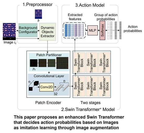
The proposed method comprises Preprocessor, a Swin Transformer+ model, and an Action model. In the first phase, the Preprocessor removes the background, including static objects such as walls, from the image and normalizes it. In this paper, “background image” refers to the image after removing dynamic objects. The module uses a Background Configurator to generate background images and Dynamic Object Extractor to preprocess the image.
Next, the Swin Transformer+ model augments the preprocessed image using Patch Encoder and two stages. The Patch Encoder partitions the preprocessed image into patches of tokens and then converts the raw pixel RGB values inside the tokens into features. The tokens are input to the first stage, which outputs features that are then transferred to the second stage and Action model. The output feature from the second stage is also transferred to the Action model.
Finally, the Action model uses a Multi-Layer Perceptron (MLP) to predict actions for a given image as a state. The features from the Swin Transformer+ model are converted into action distributions comprising multiple actions. The action with the highest probability is selected from the action distribution. The structure of the enhanced Swin Transformer model to augment the features by considering diverse arrangements of dynamic objects in each state is shown in Figure 1.
3.2. Preprocessor
The Preprocessor removes the background from the image to focus on dynamic objects, adjusts the preprocessed image size, and normalizes the raw pixel RGB values of the preprocessed image, as shown in Figure 2. The Preprocessor input is an image from an expert demonstration; the image at time step is denoted by . The input and background image are input into the Dynamic Object Extractor. The Background Configurator generates background image by leaving only static objects and removing dynamic objects one time. In this paper, objects are divided into static and dynamic objects and non-moving objects are treated as static objects. Consequently, the method generates a background image by preserving only the static objects and filling the area where dynamic objects are occupied with a background color. Dynamic Object Extractor subtracts background image from image , resulting in an image containing the entire dynamic objects. The image without the background is then resized and normalized to raw pixel RGB values. Finally, the Preprocessor outputs the preprocessed image , with only dynamic objects, as input into the Swin Transformer+ model.
The output is expressed in Equation (1):
where and denote the pixel value of the input image and background image, respectively, represents the resizing and normalization process, and H and W denote the height and width of the corresponding image, respectively.
3.3. Swin Transformer+ Model
The Patch Encoder consists of a Patch Partitioner that partitions the preprocessed image into patches and a convolutional layer that extracts features. The differences between the Swin Transformer model [22] and the proposed Swin Transformer+ model lie in the patch partitioning and embedding process. First, the image in the Swin Transformer+ model is divided into specific-sized patches considering the size of the dynamic objects clearly, whereas the Swin Transformer model determines the patch size as a hyperparameter, not considering the size of any dynamic objects. In addition, the Swin Transformer+ model uses a convolutional layer [39] instead of the linear embedding in the Swin Transformer model to extract 2D image features better.
Specifically, the patch size is determined in the Swin Transformer+ model to ensure that the patch contains one dynamic object; therefore, the preprocessed image is divided by the Patch Partitioner into n number of fixed-size patches, denoted as . The convolutional layer encodes the raw RGB pixel values into token features , as shown in Figure 3. The process of the Patch Encoder is expressed in Equation (2):
where Conv represents the convolutional layer, represents Patch Partitioner, and N denotes the total number of patches.
The two stages in the Swin Transformer+ model comprise three Swin Transformer+ Blocks to extract and augment features. The three blocks are structured as (a), (b), and (c) and contain the Padding Handler, Window Attention Processor, and MLP, as shown in Figure 4. The input of the Swin Transformer+ Block is a set of tokens . The features from each Swin Transformer+ Block are used to predict actions later, considering losses.
The number and structure of the Swin Transformer+ Block are different from those of the Swin Transformer Block. First, the number of Swin Transformer+ Blocks per stage is different because it is determined by the window size. A window [22] is a unit for locally bound tokens. Given that the window size is and that the window moves by half of the window size , it is necessary to shift the window by to create a difference in the token arrangement compared to the initial token arrangement. Therefore, the number of Swin Transformer+ Blocks is set to the number of with an additional step for the usage of the initial token arrangements.
Each Swin Transformer+ Block has a different structure. The Padding Handler is added to all Swin Transformer+ Blocks before and after the Window Attention Processor to handle the problem of uneven division of images due to the fixed patch size considering the dynamic objects. In contrast, there are no such functions of the Padding Handler in the Swin Transformer Block. The first Swin Transformer+ Block only adds the Padding Handler to the Swin Transformer Block, as shown in Figure 4a. The second Swin Transformer+ Block in the middle augments new features from the group of tokens using sequential cyclic shifts without reversal, as shown in Figure 4b, where the reversal restores the original order of tokens. The reverse is now exclusively conducted in the third Swin Transformer+ Block, as shown in Figure 4c. Thus, the order of the Swin Transformer+ Blocks is cyclic shift-cyclic shift-reverse. This differs from the Swin Transformer, which uses the order cyclic shift-reverse-cyclic shift-reverse.
The components of the Swin Transformer+ Block are described in detail below. The Padding Handler adds zero-value padding to ensure that the number of tokens in width and height is evenly divided by the window size. If the number of tokens in the width is not evenly divisible by the window size, additional column padding is required to compensate for the insufficient number of columns. Similarly, for height, any deficiency in the number of rows is compensated by additional rows. However, added paddings should not be involved in attention calculations because their objective is to assist in grouping tokens in a window rather than being involved in the attention calculation. Therefore, the added paddings must be hidden during self-attention and removed after self-attention. Consequently, the Padding Handler is positioned before and after the Window Attention Processor: first, for adding paddings, and second, for removing the added paddings. The process of Padding Handler is expressed in Equation (3):
where and denote the number of tokens in width and height, respectively, denotes the window size, denotes the number of deficiencies when dividing and by the window size , and % represents the remainder obtained after dividing the number. Additional padding is added to through n number when are not divisible by W. n is the value calculated by dividing by W and subtracting the remainder from W.
The Cyclic Shifter performs a cyclic shift starting from the second Swin Transformer+ Block in the stage. Considering the cyclic shift as data augmentation, the augmented features are generated from the second Swin Transformer+ Block. The cyclic shift can change the entire arrangement of the tokens without changing the encoded RGB pixels of each token. As each token represents a dynamic object, any change in the arrangement of the objects is seen as a form of data augmentation.
The Window Attention Processor applies the self-attention mechanism for tokens within a window and uses both a cyclic shift mask [22] and padding mask to avoid paddings and non-relevant tokens being involved in the attention mechanism. The values of the token in the window and the value of the cyclic shift mask are denoted as and , respectively, for the k-th token in the n-th window. The padding mask is generated based on the window size with a size of , where each value of the padding mask is denoted as for k-th token in n-th window. When arranging all the tokens as a matrix and grouping them into windows of length W from the top, if the padding size is greater than W, the values inside the padding mask are all filled with a large negative value. Next, if the padding and tokens are together in the window, only the portion of the padding size included within the window will have its values changed in the padding mask to a negative value. For windows where all the elements are tokens and no padding, the values inside the padding mask are all filled with 0. The padding masks prevent added paddings from being mixed into the attention score calculation by summing the padding mask values with the cyclic shift mask values. The values of the padding masks with large magnitudes are filtered through softmax to approximately 0. The parts within the mask filled with 0 remain unaffected and do not have any impact on the attention mechanism. Figure 5 shows the use of both masks. The rectangle with the yellow color represents the token, while the gray color rectangle represents added padding, and the window is delineated by a thick black border. The black and white color in the padding mask indicates value within the padding mask, respectively. Depending on whether each rectangle within the window represents padding or token, the padding mask inserts the negative value for the padding or 0 value for the token. Therefore, the black color represents the negative value, while the white color represents the value of 0. The output of the Window Attention Processor is denoted as . As is the result within a single window, the attention results of all windows within the image are aggregated as the final output.
The output of Window Attention Processor is expressed in Equations (4) and (5):
where WAP represents Window Attention Processor, denotes the softmax function, and denotes the value of cyclic shift mask.
The MLP is the same as that in the Swin Transformer in that it is used for the mixing features. By residual connection, the output feature is summed with the input of the Swin Transformer+ Block and mixed using MLP. Features are extracted per Swin Transformer+ Block, generating features owing to the blocks and i stages.
3.4. Action Model
The Action model is used to estimate action based on the features of images from the Swin Transformer+ model. The Action model contains an MLP that applies transformations and softmax to predict the actions. Because the features from each n-th Swin Transformer+ Block and i-th stage are denoted as , the augmented features are represented as . Then, all features are classified into actions. The output after applying the MLP to feature is denoted as and the action probability distribution obtained by applying softmax to is denoted as . The equation for the action probability distributions is a categorical cross-entropy loss function [40]. Finally, the loss is calculated by comparing the ground truth of action with the predicted action defined in Equation (6) where the numbers of layers and blocks are 2 and 3. The total loss is obtained by summing up each feature loss in the n-th Swin Transformer+ Block and i-th stage. The total loss is optimized using an AdamW optimizer. Although the augmented features use the same ground truth as the nonrelocated features, it is not guaranteed that they have the same correct answer as the initial state. Therefore, each loss from the augmented feature is multiplied by where N denotes the total number of augmented features, considering the Swin Transformer+ Block numbers in each stage. The weight is assigned to each loss of the augmented features by making a difference in the loss weight.
4. Experiment
This section describes the experimental details. The experiment first involved training the Swin Transformer+ model to converge using an expert demonstration dataset. Next, the Swin Transformer+ model was tested to check its accuracy and adaptation in the unobserved state. Finally, the experimental results of the Swin Transformer+, Swin Transformer model, Decision Transformer model, and Vision Transformer model [41] were compared.
4.1. Datasets
To verify the proposed method, Atari [42]-based path planning was utilized. For the experiments, a grand challenge dataset [43] was used. This dataset contains 1,779,771 images and 384 trajectories. The trajectories consisted of sequential image numbers, rewards, terminal information, and actions. The trajectories were divided based on episodes. The number of images used for training was 9216, each with a size of 210 × 160 × 3. Of the total number of images, 90% were used for training the model and 10% were used for validation. The distribution of the actions in the training images is presented in Table 2.
4.2. Experimental Environments
The hyperparameters of the proposed method are listed in Table 3. The input was a single RGB image of 252 × 234 (height × width) after preprocessing. Each image was labeled with actions from the stored trajectory as the ground truth. The common patch size was defined as 18 × 13 (height × width) to contain a dynamic object, such as a pellet, in a divided image. The patch partition splits the image into grids of 18 rows and 13 columns and crops the sides of the preprocessed image by 9 pixels.
The window size was fixed at three and the window size unit was based on the number of patches. The window size is a hyperparameter, considering the padding size and the patch size. The total number of patches is divided twice with the same window size. The first division is performed using the input of the total number of patches, and the second division is performed after patch merging. Patch merging [22] increases the patch size; however, it decreases the total number of patches by half. The decreased number of patches must be further divided with the same window size. Padding is a tool used to complement cases where the number of patches is not divisible by the window size. However, because padding can introduce noise, only the minimum amount of padding is added. Consequently, window size 3 is determined by the greatest common divisor of the combined total number of patches and paddings. The stage of the proposed method was defined as three Swin Transformers+ Blocks with outputs of 32 and 128 dimensions. At each stage, the dimensions were increased by a factor of four. Considering the pellet size, which was originally 2 × 4 pixels in the raw input image, the dimensions were set to 32, four times the original pellet size, to capture its representation. The total number of classes was four, the same as the action types in the environment. The number of Swin Transformer+ Block was only three, which means there are three Swin Transformer+ Blocks in each stage, and the number of output features was three. The number of blocks was considered to balance the distortion caused by the cyclic shift. Hyperparameters, such as dropout, batch size, learning rate, and total training epochs, were also included.
The experiments were conducted on a Windows 10, i5-9400 processor, NVIDIA GeForce GTX 1050 2 GB graphics card, and 32 GB DDR4 memory. The proposed method was created using Python version 3.7.13, and PyTorch 1.8.0 was utilized to implement data preprocessing and imitation learning with Swin Transformer+ for data augmentation.
4.3. Experimental Results
Figure 6 shows the training and validation losses of the proposed method. The training loss of the proposed method started at 1.24068, decreased to 0.41616, and then converged. This indicates that training for up to 92 epochs is necessary for convergence because the lowest loss was recorded at 0.00587. The figure also shows the change in validation loss. The initial validation loss of 1.24068 decreased to 0.68185. In the 89th epoch, the model achieved the lowest validation loss of 0.56141 for the validation dataset.
Figure 7 shows the accuracy of the proposed method during training and validation. The initial accuracy for training was 30% but increased to 82%. Similarly, the validation accuracy was 34% but reached approximately 81.5% after 100 epochs. However, the highest validation accuracy 86.4% was achieved after 93 epochs. Based on these results, it was assumed that overfitting occurred during the training process, leading to training results up to epoch 90 as the optimal model. Therefore, it was verified that the proposed method with augmented features helps learn experts’ control patterns through cyclic shifts and dynamic object arrangement, thereby increasing accuracy.
The masks for the total tokens and padding are shown in Figure 8. The values of the mask were different at each stage, depending on the number of tokens for padding added to the tokens of the mask. The masks shown below were those used in the second stage: Figure 8a shows masks for the total tokens. When the mask in Figure 8a is partitioned with window size and converted to a matrix for self-attention calculation, it results in a cyclic shift mask that is required for the attention process to prevent nonadjacent tokens from being calculated together in the attention calculation. The purple color in Figure 8a represents 0 value and other colors all represent positive values with only a difference in magnitude of value. The values of the cyclic shift mask go through the filtering process where 0 remains 0, and all non-zero values convert to minus 100 values. The cyclic shift mask inserts 0 value for the padding location since the padding value is blocked by the padding mask. Figure 8b shows a mask for the paddings covered with a mask such that the paddings are not processed in the attention calculation. The padding mask in Figure 8b shows one of masks at the boundary of tokens. The purple color in Figure 8b represents a negative value for paddings in the self-attention mechanism, while the yellow color represents 0 value for tokens.
The proposed method was compared with a Swin Transformer, Decision Transformer, and Vision Transformer models. The accuracy and generalization performance were compared, as shown in Table 4. To confirm the accuracy, we compare the action-estimated results with the Swin Transformer, Decision Transformer, Vision Transformer, and Swin Transformer+ models. Using the images stored in the training images, experimental comparison models output action prediction distributions that are compared with the action labels. Generalization was tested when encountering situations outside the training dataset and compared the earned scores between the models. When evaluated after training with the same images, the accuracies of the Swin Transformer and Vision Transformer models were higher than that of the proposed method by 11.6% and 8.7%, respectively. However, the accuracy of the Decision Transformer was low compared to other models in comparison. This is because Decision Transformer focuses on identifying the most optimal action related to the result rather than replicating the exact same action as the expert for the next step. Next, the best evaluation score, measured by considering the moving path automatically, with the proposed method was 920, higher than that with the Swin Transformer model. Furthermore, the proposed method had scores of 1020 and 1200, a higher score than Decision Transformer model and Vision Transformer model. The average evaluation score of the proposed method was 226, higher than that of the Swin Transformer model, and 35 and 59, higher than the Decision Transformer model and Vision Transformer model. The results indicated that the performance of the proposed method was better than that of the experimental comparison models. Although the accuracy was lower, using the cyclic shift as an augmentation approach improved the imitation learning performance in an actual environment. The Swin Transformer+ model was robust to variations in the object arrangement by augmenting various features. This demonstrates the improvements in the generalization performance and the possibility of increased robustness in diverse images with the proposed method.
5. Conclusions
We proposed imitation learning using a Swin Transformer+ model based on images. The proposed method utilized the Swin Transformer+ model, Preprocessor, and Action model to augment the images considering the diverse arrangements of objects. The actions were predicted using augmented images, which were then compared to action labels. The proposed method was evaluated for its capacity to learn an expert’s control pattern from augmented images, using accuracy as an evaluation metric. Additionally, an experiment was conducted to measure the best evaluation score using the proposed method. It was confirmed that the Swin Transformer+ model performed better than the Swin Transformer model and other comparison models in an actual environment. The proposed method outperformed its counterparts with higher best and average evaluation scores, respectively, than the other comparison models with the Preprocessor and Action models. The limitation of the proposed method is that it is difficult to adjust the parameters according to the environment due to the complexity of the structure of the Swin Transformer model. Therefore, the challenge of this paper is to develop an automated method for adjusting parameters such as window size and patch size according to various environments since the parameters require detailed adjustments. Furthermore, the importance of quality expert dataset is a challenge because the training is based on expert annotations.
In future research, it will be possible to develop an approach that can adapt to complex scenarios with many objects and dynamic objects of various shapes. In addition, additional augmentation techniques that can be used with cyclic shifts for imitation learning should be investigated.
Author Contributions
Conceptualization, Y.P. and Y.S.; methodology, Y.P. and Y.S.; software, Y.P. and Y.S.; validation, Y.P. and Y.S.; writing—review and editing, Y.P. and Y.S.; supervision, Y.S.; project administration, Y.S.; funding acquisition, Y.S. All authors have read and agreed to the published version of the manuscript.
Funding
This research was supported by the Culture, Sports and Tourism R&D Program through the Korea Creative Content Agency grant funded by the Ministry of Culture, Sports and Tourism in 2023 (Project Name: Education & research group for advanced AI technology in the field of sports games, Project Number: R2022020003, Contribution Rate: 100%).
Data Availability Statement
Data are available in a publicly accessible repository that does not issue DOIs. Publicly available datasets were analyzed in this thesis. These data can be found here: https://github.com/yobibyte/atarigrandchallenge, accessed on 13 April 2023.
Conflicts of Interest
The authors declare no conflict of interest.
References
- Jiang, Z.; Li, S.; Sung, Y. Enhanced Evaluation Method of Musical Instrument Digital Interface Data based on Random Masking and Seq2Seq Model. Mathematics 2022, 10, 2747. [Google Scholar] [CrossRef]
- Song, W.; Li, D.; Sun, S.; Zhang, L.; Yu, X.; Choi, R.; Sung, Y. 2D&3DHNet for 3D Object Classification in LiDAR Point Cloud. Remote Sens. 2022, 14, 3146. [Google Scholar] [CrossRef]
- Yoon, H.; Li, S.; Sung, Y. Style Transformation Method of Stage Background Images by Emotion Words of Lyrics. Mathematics 2021, 9, 1831. [Google Scholar] [CrossRef]
- Balakrishna, A.; Thananjeyan, B.; Lee, J.; Li, F.; Zahed, A.; Gonzalez, J.E.; Goldberg, K. On-policy robot imitation learning from a converging supervisor. In Proceedings of the 3rd Conference on Robot Learning (CoRL), Virtual, 16–18 November 2020; pp. 24–41. [Google Scholar]
- Jang, E.; Irpan, A.; Khansari, M.; Kappler, D.; Ebert, F.; Lynch, C.; Levine, S.; Finn, C. BC-Z: Zero-shot task generalization with robotic imitation learning. In Proceedings of the 5th Conference on Robot Learning (CoRL), Auckland, New Zealand, 14–18 December 2022; pp. 991–1002. [Google Scholar]
- Codevilla, F.; Müller, M.; López, A.; Koltun, V.; Dosovitskiy, A. End-to-end driving via conditional imitation learning. In Proceedings of the IEEE International Conference on Robotics and Automation (ICRA), Brisbane, Australia, 21–26 May 2018; pp. 4693–4700. [Google Scholar]
- Kebria, P.M.; Khosravi, A.; Salaken, S.M.; Nahavandi, S. Deep Imitation Learning for Autonomous Vehicles based on Convolutional Neural Networks. IEEE/CAA J. Autom. Sin. 2020, 7, 82–95. [Google Scholar] [CrossRef]
- Zhifei, S.; Meng Joo, E. A Survey of Inverse Reinforcement Learning Techniques. Int. J. Intell. Comput. Cybern. 2012, 5, 293–311. [Google Scholar] [CrossRef]
- Torabi, F.; Warnell, G.; Stone, P. Behavioral Cloning from Observation. arXiv 2018, arXiv:1805.01954. [Google Scholar]
- Ross, S.; Bagnell, D. Efficient reductions for imitation learning. In Proceedings of the 13th International Conference on Artificial Intelligence and Statistics (AISTATS), Sardinia, Italy, 13–15 May 2010; pp. 661–668. [Google Scholar]
- Taylor, L.; Nitschke, G. Improving deep learning with generic data augmentation. In Proceedings of the 2018 IEEE Symposium Series on Computational Intelligence (SSCI), Bengaluru, India, 18–21 November 2018; pp. 1542–1547. [Google Scholar]
- Zhong, Z.; Zheng, L.; Kang, G.; Li, S.; Yang, Y. Random erasing data augmentation. In Proceedings of the 34th AAAI Conference on Artificial Intelligence, New York, NY, USA, 7–12 February 2020; pp. 13001–13008. [Google Scholar]
- Nanni, L.; Paci, M.; Brahnam, S.; Lumini, A. Feature Transforms for Image Data Augmentation. Neural Comput. Appl. 2022, 34, 22345–22356. [Google Scholar] [CrossRef]
- Gong, C.; Ren, T.; Ye, M.; Liu, Q. Maxup: Lightweight adversarial training with data augmentation improves neural network training. In Proceedings of the IEEE/CVF Conference on Computer Vision and Pattern Recognition (CVPR), Virtual, 19–25 June 2021; pp. 2474–2483. [Google Scholar]
- Zheng, X.; Chalasani, T.; Ghosal, K.; Lutz, S.; Smolic, A. STaDA: Style Transfer as Data Augmentation. arXiv 2019, arXiv:1909.01056. [Google Scholar]
- Goodfellow, I.; Pouget-Abadie, J.; Mirza, M.; Xu, B.; Warde-Farley, D.; Ozair, S.; Courville, A.; Bengio, Y. Generative adversarial nets. In Proceedings of the 28th Advances in Neural Information Processing Systems (NIPS), Montréal, QC, Canada, 8–13 December 2014; pp. 1–9. [Google Scholar]
- Huang, S.W.; Lin, C.T.; Chen, S.P.; Wu, Y.Y.; Hsu, P.H.; Lai, S.H. AugGAN: Cross domain adaptation with GAN-based data augmentation. In Proceedings of the 15th European Conference on Computer Vision (ECCV), Munich, Germany, 8–14 September 2018; pp. 718–731. [Google Scholar]
- Dornaika, F.; Sun, D.; Hammoudi, K.; Charafeddine, J.; Cabani, A.; Zhang, C. Object-centric Contour-aware Data Augmentation Using Superpixels of Varying Granularity. Pattern Recognit. 2023, 139, 109481–109493. [Google Scholar] [CrossRef]
- Knyazev, B.; Cătălina Cangea, H.; Aaron Courville, G.W.T.; Belilovsky, E. Generative compositional augmentations for scene graph prediction. In Proceedings of the IEEE/CVF International Conference on Computer Vision (ICCV), Montreal, QC, Canada, 11–17 October 2021; pp. 15827–15837. [Google Scholar]
- Yin, Z.; Gao, Y.; Chen, Q. Structural generalization of visual imitation learning with position-invariant regularization. In Proceedings of the 11th International Conference on Learning Representations (ICLR), Kigali, Rwanda, 1–5 May 2023; pp. 1–14. [Google Scholar]
- Zhang, L.; Wen, T.; Min, J.; Wang, J.; Han, D.; Shi, J. Learning object placement by inpainting for compositional data augmentation. In Proceedings of the European Conference on Computer Vision (ECCV), Virtual, 23–28 August 2020; pp. 566–581. [Google Scholar]
- Liu, Z.; Lin, Y.; Cao, Y.; Hu, H.; Wei, Y.; Zhang, Z.; Lin, S.; Guo, B. Swin transformer: Hierarchical vision transformer using shifted windows. In Proceedings of the 21st IEEE/CVF International Conference on Computer Vision (ICCV), Virtual, 11–17 October 2021; pp. 10012–10022. [Google Scholar]
- Sasaki, F.; Yamashina, R. Behavioral cloning from noisy demonstrations. In Proceedings of the 9th International Conference on Learning Representations (ICLR), Virtual, 3–7 May 2021; pp. 1–14. [Google Scholar]
- Codevilla, F.; Santana, E.; López, A.M.; Gaidon, A. Exploring the limitations of behavior cloning for autonomous driving. In Proceedings of the 2019 IEEE/CVF International Conference on Computer Vision (CVPR), Long Beach, CA, USA, 16–20 June 2019; pp. 9329–9338. [Google Scholar]
- He, K.; Zhang, X.; Ren, S.; Sun, J. Deep residual learning for image recognition. In Proceedings of the IEEE Conference on Computer Vision and Pattern Recognition (CVPR), Las Vegas, NV, USA, 26 June–1 July 2016; pp. 770–778. [Google Scholar]
- Yu, T.; Finn, C.; Xie, A.; Dasari, S.; Zhang, T.; Abbeel, P.; Levine, S. One-Shot Imitation from Observing Humans via Domain-Adaptive Meta-Learning. arXiv 2018, arXiv:1802.01557. [Google Scholar]
- Bronstein, E.; Palatucci, M.; Notz, D.; White, B.; Kuefler, A.; Lu, Y.; Paul, S.; Nikdel, P.; Mougin, P.; Chen, H.; et al. Hierarchical model-based imitation learning for planning in autonomous driving. In Proceedings of the 2022 IEEE/RSJ International Conference on Intelligent Robots and Systems (IROS), Kyoto, Japan, 23–27 October 2022; pp. 8652–8659. [Google Scholar]
- Chen, L.; Lu, K.; Rajeswaran, A.; Lee, K.; Grover, A.; Laskin, M.; Abbeel, P.; Srinivas, A.; Mordatch, I. Decision transformer: Reinforcement learning via sequence modeling. In Proceedings of the 2021 Advances in Neural Information Processing Systems (NIPS), Virtual, 6–14 December 2021; pp. 15084–15097. [Google Scholar]
- Laskey, M.; Lee, J.; Fox, R.; Dragan, A.; Goldberg, K. DART: Noise injection for robust imitation learning. In Proceedings of the 1st Annual Conference on Robot Learning (CoRL), Mountain View, CA, USA, 13–15 November 2017; pp. 143–156. [Google Scholar]
- Mnih, V.; Kavukcuoglu, K.; Silver, D.; Rusu, A.; Veness, J.; Bellemare, M.; Graves, A.; Riedmiller, M.; Fidjeland, A.; Ostrovski, G. Human–level control through deep reinforcement learning. Nature 2015, 518, 529–533. [Google Scholar] [CrossRef] [PubMed]
- Kelly, M.; Sidrane, C.; Driggs-Campbell, K.; Kochenderfer, M.J. HG-DAgger: Interactive imitation learning with human experts. In Proceedings of the International Conference on Robotics and Automation (ICRA), Montreal, QC, Canada, 20–24 May 2019; pp. 8077–8083. [Google Scholar]
- Ross, S.; Gordon, G.; Bagnell, D. A reduction of imitation learning and structured prediction to no-regret online learning. In Proceedings of the 14th International Conference on Artificial Intelligence and Statistics (AISTATS), Fort Lauderdale, FL, USA, 11–13 April 2011; pp. 627–635. [Google Scholar]
- Yan, C.; Qin, J.; Liu, Q.; Ma, Q.; Kang, Y. Mapless Navigation with Safety-enhanced Imitation Learning. IEEE Trans. Ind. Electron. 2022, 70, 7073–7081. [Google Scholar] [CrossRef]
- Galashov, A.; Merel, J.S.; Heess, N. Data augmentation for efficient learning from parametric experts. In Proceedings of the 39th Advances in Neural Information Processing Systems (NIPS), New Orleans, LA, USA, 28 November–9 December 2022; pp. 31484–31496. [Google Scholar]
- Zhu, Y.; Joshi, A.; Stone, P.; Zhu, Y. VIOLA: Imitation Learning for Vision-Based Manipulation with Object Proposal Priors. arXiv 2022, arXiv:2210.11339. [Google Scholar]
- Antotsiou, D.; Ciliberto, C.; Kim, T.K. Adversarial imitation learning with trajectorial augmentation and correction. In Proceedings of the IEEE International Conference on Robotics and Automation (ICRA), Xi’an, China, 30 May–5 June 2021; pp. 4724–4730. [Google Scholar]
- Ho, J.; Ermon, S. Generative adversarial imitation learning. In Proceedings of the 30th Advances in Neural Information Processing Systems (NIPS), Barcelona, Spain, 5–10 December 2016; pp. 1–9. [Google Scholar]
- Pfrommer, D.; Zhang, T.; Tu, S.; Matni, N. TaSIL: Taylor series imitation learning. In Proceedings of the 36th Advances in Neural Information Processing Systems (NeurlPS), New Orleans, LA, USA, 28 November–9 December 2022; pp. 20162–20174. [Google Scholar]
- GitHub—Microsoft/Swin-Transformer: This Is an Official Implementation for “Swin Transformer: Hierarchical Vision Transformer Using Shifted Windows”. Available online: https://github.com/microsoft/Swin-Transformer (accessed on 29 December 2022).
- Zhang, Z.; Sabuncu, M. Generalized cross entropy loss for training deep neural networks with noisy labels. In Proceedings of the 32nd Advances in Neural Information Processing Systems (NIPS), Montréal, QC, Canada, 2–8 December 2018; pp. 8778–8788. [Google Scholar]
- Dosovitskiy, A.; Beyer, L.; Kolesnikov, A.; Weissenborn, D.; Zhai, X.; Unterthiner, T.; Dehghani, M.; Minderer, M.; Heigold, G.; Gelly, S.; et al. An Image is Worth 16x16 Words: Transformers for Image Recognition at Scale. arXiv 2020, arXiv:2010.11929. [Google Scholar]
- Mnih, V.; Kavukcuoglu, K.; Silver, D.; Graves, A.; Antonoglou, I.; Wierstra, D.; Riedmiller, M. Playing Atari with Deep Reinforcement Learning. arXiv 2013, arXiv:1312.5602. [Google Scholar]
- Kurin, V.; Nowozin, S.; Hofmann, K.; Beyer, L.; Leibe, B. The Atari Grand Challenge Dataset. arXiv 2017, arXiv:1705.10998. [Google Scholar]
Figure 1.
Swin Transformer+ -based imitation learning.

Figure 2.
The process of Preprocessor.

Figure 3.
Process of Patch Encoder.

Figure 4.
The configuration of Swin Transformer+ Blocks, in order from above (a–c): (a) first Swin Transformer+ Block in stage; (b) second Swin Transformer+ Block in stage; (c) last Swin Transformer+ Block in stage.
Figure 4.
The configuration of Swin Transformer+ Blocks, in order from above (a–c): (a) first Swin Transformer+ Block in stage; (b) second Swin Transformer+ Block in stage; (c) last Swin Transformer+ Block in stage.

Figure 5.
Process of Window Attention Processor. Cyclic shift mask is from Liu, Z.+2021 [22].
Figure 5.
Process of Window Attention Processor. Cyclic shift mask is from Liu, Z.+2021 [22].

Figure 6.
Training and validation loss of Swin Transformer+.

Figure 7.
Training and validation accuracy of Swin Transformer+.

Figure 8.
Masks for cyclic shift and padding: (a) mask for cyclic shift; (b) mask for padding.


Table 1.
Comparison between imitation learning research and the proposed method.
| Research | Deep Learning Architecture | Augmentation Method | Spatial Relation |
|---|---|---|---|
| DART [29] | DQN | Noise Generator | × |
| HG-Dagger [31] | - | Data Aggregation | × |
| CAT and DAugGI [36] | GAIL | Adversarial Method | × |
| TaSIL [38] | - | Taylor Series | × |
| Decision Transformer [28] | GPT | - | × |
| The Proposed Method | Swin Transformer | Cyclic Shift | √ |
Table 2.
Actions distribution of dataset.
| Actions | Up | Right | Left | Down |
|---|---|---|---|---|
| Total Number | 1875 | 2283 | 2687 | 2371 |
Table 3.
Hyper parameters for Swin Transformer+.
| Hyper Parameter | Value |
|---|---|
| Image size | (252, 234) |
| Patch size | (18, 13) |
| Input channels | 3 |
| Classes | 4 |
| 1st Stage Embedding dimension | 32 |
| 2nd Stage Embedding dimension | 128 |
| Swin Transformer+ Block number | [3, 3] |
| Multi-Head number | [4, 4] |
| Window size | 3 |
| Dropout rate | 0.5 |
| Epochs | 100 |
| Learning rate | 0.0003 |
| Batch size | 16 |
Table 4.
Comparison with other models.
| Model | Accuracy (%) | Best Eval. Score | Avg. Eval. Score |
|---|---|---|---|
| The Proposed Method | 86.4% | 1700 | 286 |
| Preprocessor + Swin Transformer model + Action model | 98% | 780 | 60 |
| Preprocessor + Vision Transformer model + Action model | 95.1% | 500 | 227 |
| Preprocessor + Decision Transformer model + Action model | 23.6% | 680 | 251 |
Disclaimer/Publisher’s Note: The statements, opinions and data contained in all publications are solely those of the individual author(s) and contributor(s) and not of MDPI and/or the editor(s). MDPI and/or the editor(s) disclaim responsibility for any injury to people or property resulting from any ideas, methods, instructions or products referred to in the content. |
© 2023 by the authors. Licensee MDPI, Basel, Switzerland. This article is an open access article distributed under the terms and conditions of the Creative Commons Attribution (CC BY) license (https://creativecommons.org/licenses/by/4.0/).
Share and Cite
MDPI and ACS Style
Park, Y.; Sung, Y. Imitation Learning through Image Augmentation Using Enhanced Swin Transformer Model in Remote Sensing. Remote Sens. 2023, 15, 4147. https://doi.org/10.3390/rs15174147
AMA Style
Park Y, Sung Y. Imitation Learning through Image Augmentation Using Enhanced Swin Transformer Model in Remote Sensing. Remote Sensing. 2023; 15(17):4147. https://doi.org/10.3390/rs15174147
Chicago/Turabian StylePark, Yoojin, and Yunsick Sung. 2023. "Imitation Learning through Image Augmentation Using Enhanced Swin Transformer Model in Remote Sensing" Remote Sensing 15, no. 17: 4147. https://doi.org/10.3390/rs15174147
Note that from the first issue of 2016, this journal uses article numbers instead of page numbers. See further details here.