Exploring the Relationship between Temporal Fluctuations in Satellite Nightlight Imagery and Human Mobility across Africa

Abstract

Mobile phone data have been increasingly used over the past decade or more as a pretty reliable indicator of human mobility to measure population movements and the associated changes in terms of population presence and density at multiple spatial and temporal scales. However, given the fact mobile phone data are not available everywhere and are generally difficult to access and share, mostly because of commercial restrictions and privacy concerns, more readily available data with global coverage, such as night-time light (NTL) imagery, have been alternatively used as a proxy for population density changes due to population movements. This study further explores the potential to use NTL brightness as a short-term mobility metric by analysing the relationship between NTL and smartphone-based Google Aggregated Mobility Research Dataset (GAMRD) data across twelve African countries over two periods: 2018–2019 and 2020. The data were stratified by a measure of the degree of urbanisation, whereby the administrative units of each country were assigned to one of eight classes ranging from low-density rural to high-density urban. Results from the correlation analysis, between the NTL Sum of Lights (SoL) radiance values and three different GAMRD-based flow metrics calculated at the administrative unit level, showed significant differences in NTL-GAMRD correlation values across the eight rural/urban classes. The highest correlations were typically found in predominantly rural areas, suggesting that the use of NTL data as a mobility metric may be less reliable in predominantly urban settings. This is likely due to the brightness saturation and higher brightness stability within the latter, showing less of an effect than in rural or peri-urban areas of changes in brightness due to people leaving or arriving. Human mobility in 2020 (during COVID-19-related restrictions) was observed to be significantly different than in 2018–2019, resulting in a reduced NTL-GAMRD correlation strength, especially in urban settings, most probably because of the monthly NTL SoL radiance values remaining relatively similar in 2018–2019 and 2020 and the human mobility, especially in urban settings, significantly decreasing in 2020 with respect to the previous considered period. The use of NTL data on its own to assess monthly mobility and the associated fluctuations in population density was therefore shown to be promising in rural and peri-urban areas but problematic in urban settings.

1. Introduction

The acquisition of data pertaining to human mobility and presence is of critical importance within numerous fields of research for producing socioeconomic and development indicators, estimating greenhouse gas emissions, mapping urban extents, and assessing the spread, prevalence, and incidence of various human diseases, among others, driving a demand to refine the processes by which these mobility metrics are measured. With rates of human mobility increasing in their volumes and reach at both global and local scales, methods and datasets for quantifying them, particularly in data-sparse middle- and low-income settings, are becoming an important need. Moreover, with seasonal changes in human mobility that drive disease dynamics (Grenfell et al., 2001; Wesolowski et al., 2012; Wesolowski, Metcalf et al., 2015; Wesolowski, Qureshi et al., 2015) [1,2,3,4] the demand for resources (Steele et al., 2021) [5] and impact infrastructure planning needs (Strano et al., 2018) [6] can be particularly challenging to quantify (Lai et al., 2022; Mao et al., 2015; Song et al., 2021; Woods et al., 2022) [7,8,9,10]. Since its public distribution in recent decades, satellite-derived night-time light (NTL) imagery has proved itself a reliable proxy of human presence, where large bright areas correspond to higher populations compared to dimly lit areas (Bharti and Tatem, 2018; Bharti et al., 2011; Bustos, 2015) [11,12,13]. Furthermore, NTL imagery has been used as a global indicator of anthropogenic activity and development (Elvidge et al., 2012) [14] and, due to its historical availability and regular acquisition, enables comparative studies to be made over both short and long time periods (Doll et al., 2000; Ebener et al., 2005) [15,16]. As the technology has matured, so has the quality and availability of the NTL data for the scientific and operational communities with the new Visible Infrared Imaging Radiometer Suite (VIIRS) instrument, aboard the joint National Aeronautics and Space Administration (NASA) and National Oceanic and Atmospheric Administration (NOAA) Suomi National Polar-orbiting Partnership (Suomi NPP) and NOAA-20 satellites, offering several refinements compared to the older Defense Meteorological Satellite Program-Operational Linescan System (DMSP-OLS), such as increased spatial resolution of both the Ground Instantaneous Field of View (i.e., 0.55 versus 25 km² at Nadir) and the corresponding generated global grids (i.e., 15 versus 30 arc-second grid cell corresponding to ~500 m versus ~1 km at the equator) and temporal resolution (i.e., monthly versus annual) of cloud-free composites, as well as the full filtering of data impacted by stray light (Elvidge et al., 2013) [17].

Previous research has highlighted the potential of multi-temporal NTL imagery for measuring changes in population presence and density over time as a result of mobility. This has included seasonal labour migration into towns and cities in the Sahel region of Africa (Lai, Farnham et al., 2019) [18] and its impact on infectious disease dynamics (Bharti et al., 2011) [12], net migration at NUTS III level in Europe (Chen 2020) [19], seasonal flows of tourists (Stathakis and Baltas, 2018; Tselios and Stathakis, 2020) [20,21], COVID-19 lockdown in global megacities (Xu, et al., 2021) [22], and induced displacement (Lu et al., 2016) [23].

In each case, while the evidence is clear on NTL data capturing aspects of population presence and density changes induced by mobility, there are often other factors, such as disaster- or conflict-induced power outages (Montoya-Rincon et al., 2022) [24], that can be hard to disentangle, and thus, translation into quantitative direct measures of mobility can be challenging. Moreover, the saturation of brightness values in highly urbanised settings can also affect the relationship between changes in brightness, or lack thereof, and mobility. To improve our understanding of the value of NTL data for assessing human mobility and the associated changes in population presence and density, comparisons with alternative datasets are required.

Data on the aggregated movements of mobile phones over time have often been shown to be a reliable and accurate source of quantitative estimates of human movement patterns from subnational to global scales (Lai, Farnham et al., 2019; Lai, zu Erbach-Schoenberg et al., 2019; Ruktanonchai et al., 2018) [18,25,26]. Such data are typically obtained and derived either from Call Detail Records (CDRs), whereby anonymized and aggregated billing records of communications routed through cell towers are measured (Bengtsson et al., 2011; Buckee et al., 2013; Ruktanonchai et al., 2016) [27,28,29], or from aggregations of smartphone-derived GPS location data (Lai, zu Erbach-Schoenberg et al., 2019; Ruktanonchai et al., 2018) [25,26]. Each has their own set of biases and uncertainties, which impact the accuracy and reliability of the assessed human mobility patterns (Lai, zu Erbach-Schoenberg et al., 2019) [25]. The Google Aggregated Mobility Research Dataset (GAMRD) data, providing a measurement of human movements as quantized flow metrics, are principally derived from smartphones and represent the result of anonymous and aggregated phone locations for users who have opted into Google’s Location History feature, which is off by default (Ruktanonchai et al., 2018) [26]. Previous research has indicated that there is a strong nonlinear relationship between GAMRD and NTL data (Dickinson et al., 2020) [30]. However, these studies only obtained and analysed mobility data for a short time period (e.g., 6–12 months) in a single country. The degree to which this relationship varies across locations and degrees of urbanisation has not been explored, particularly in low- and middle-income settings and at the monthly timescale. Based on multiple-year (2018–2020) and large-scale mobility data and NTL data at fine spatial resolution across 12 African countries, the current study seeks to address this through (i) examining the NTL-GAMRD relationship across Africa for two time periods (i.e., 2018/19 and 2020) and (ii) determining how the degree of urbanisation affects the correlations.

2. Materials and Methods

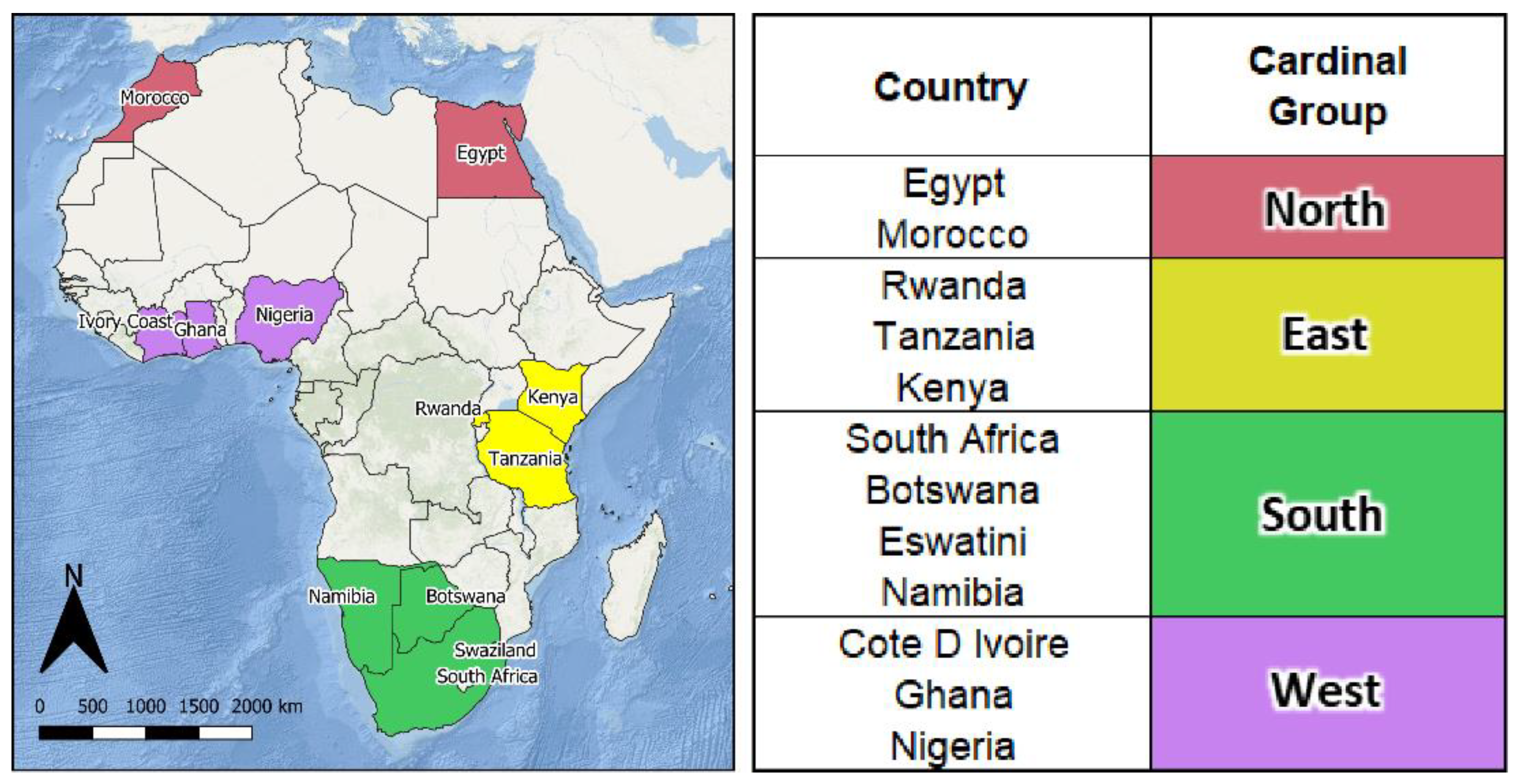
The GAMRD data contain anonymized mobility flows aggregated over users who have turned on their Location History setting that is off by default. The dataset aggregates flows between S2 cells which are here further aggregated by the level 2 administrative unit of origin and destination within and between 12 African countries (Figure 1).

To produce this dataset, machine learning is applied to log data to automatically segment it into semantic “trips” (Bassolas et al., 2019) [31]. To provide strong privacy guarantees, all trips are anonymized and aggregated using a differentially private mechanism (Wilson et al., 2020) [32] to aggregate flows over time (Google, n.d.) [33]. This research was carried out on the resulting heavily aggregated and differentially private data. No individual user data was ever manually inspected; only heavily aggregated flows of large populations were handled.

All anonymized trips are processed in aggregate to extract their origin and destination location and time. For example, if users travelled from location A to location B within time interval t, the corresponding cell (A, B, t) in the tensor would be n∓err, where err is Laplacian noise. The automated Laplace mechanism adds random noise drawn from a zero-mean Laplace distribution and yields a (𝜖, δ)-differential privacy guarantee of 𝜖 = 0.66 and δ = 2.1 × 10⁻²⁹ per metric. Specifically, for each week W and each location pair (A, B), the number of unique users who took a trip from location A to location B during week W is calculated. To each of these metrics, Laplace noise from a zero-mean distribution of scale 1/0.66 is added. All metrics for which the noisy number of users is lower than 100 are removed, following the process described in (Wilson et al., 2020) [32], and the rest are published. This yields that each published metric satisfies (𝜖, δ)-differential privacy with values defined above. The parameter 𝜖 controls the noise intensity in terms of its variance, while δ represents the deviation from pure 𝜖-privacy. The closer they are to zero, the stronger the privacy guarantees.

The GAMRD dataset used in this study covered the years 2018, 2019, and 2020 and initially contained weekly data representing relative population flows which were subsequently aggregated to a monthly timescale to allow direct comparison with the monthly VIIRS NTL data. The GAMRD data for 2020 were initially supplied in S2 Geometry (S2 Geometry, 2018) [34] and were then converted to the GCS-WGS84 coordinate system. Based on the origin and destination coordinates of the trips and using shapefiles representing level 2 administrative units, the relative flows were aggregated into 3 unique GAMRD-based flow metrics (i.e., internal flow, inward flow, and outward flow) as described in

Table 1. The three Google Location History Flow Metrics created for the current study based on the direction and nature of movement within and between level 2 administrative units.

GAMRD Flow Metric	Description
Internal Flow	The internal flow within the same administrative unit (as this value increases, population total is unchanged but is more mobile)
Inward Flow	The external flow to the administrative units from others either within the same country or abroad (as this value increases, population within this admin unit increases)
Outward Flow	The external flow increases, population within this admin unit decreases)

. Therefore, for every level 2 administrative unit of each country of interest, three distinct GAMRD-based flow metrics were available for each month over the study period (i.e., 2018–2020).

Although it would have been preferable to combine GAMRD data from all years (i.e., 2018, 2019, and 2020), this was not possible due to the different spatial aggregation methods used to produce them, and so the study results were necessarily split into two time-periods: 2018/19 and 2020. The 2018/19 data represented flows originally calculated between S2 cells whilst the 2020 data were originally provided based on 1 km cells in WGS84. Although both groups were later reformatted to represent flows between level 2 administrative units in GCS-WGS84, the machine learning-based algorithm used to calculate the raw flows produced two unique datasets that can be justifiably compared to each other and to other data (namely, the VIIRS-NTL data in this study) but cannot be directly combined. Finally, the data referring to December 2019 were removed due to quality issues.

A Python script (Py v3.6) was created to download and extract VIIRS-NTL imagery for each country of interest and thereafter apply postprocessing stages in preparation for zonal statistics. The NTL data were provided by the Colorado School of Mines as monthly composites in geotiff format with the globe divided into 6 tiles (Elvidge et al., 2017) [35]. Monthly composites were filtered to exclude data impacted by stray light, lightning, lunar illumination, and cloud-cover where the monthly series is run globally using two different configurations. The first excludes any data impacted by stray light. The second includes these data if the radiance values have undergone the stray-light correction procedure. These two configurations, one of which includes the stray-light corrected data, will have more data coverage toward the poles, but will be of reduced quality with the decision of which configuration to use being dependent on the context. For each of the months from 2012–2020, for the monthly non-tiled versions, the annual masks for each year were applied to all the months for that year. For example, the 2020 lit mask was applied on all the months of 2020 (Mills et al., 2013) [36]. According to Elvidge et al. (2013) [17], in contrast to the DMSP overpass time which is near 7.30 pm, the SNPP overpass time is near 1.30 am and peak lighting is prior to 10 pm (after which there is some decline in the quantity of outdoor lighting, but we also agree with Eldvige et al. (2013) [17] that VIIRS data strongly indicate that there is still plenty of lighting being detected after midnight which may or may not only link to public infrastructure lights). After using the annual composites for removing ephemeral lights (unrelated to electric lighting) and background (non-lights) from monthly composites which were already processed for removing persistent gas flares, as well as the impact of sunlit, moonlit, stray lights, lightening, high energy particle, overglow, and cloud-cover, the monthly composites should only include electric lights, which may or may not be related to population presence and thus be affected by human mobility in various ways in different contexts (i.e., urban, peri-urban, vs. rural). At the time of the study design and data analysis (mid-2019), VIIRS annual composite data were not available for all three years of 2018–2020, and only the data that were available up until 2016 had been postprocessed to remove ephemeral lights, such as volcanic activity, fires, and atmospheric noise (Elvidge et al., 2017) [35]. However, the version 1 series of the monthly composites were not filtered to screen out lights from aurora, fires, boats, and other non-residential lights, thus requiring additional postprocessing (Li et al., 2013; Wang et al., 2017) [37,38]. The downloaded files were composed of a primary radiance raster (*rade9.tif) containing floating-point radiance values with units in nanoWatts/cm²/sr and a corresponding coverage raster (*cvg.tif) of integer values representing the number of observations made on each pixel in each month to be used for quality control.

After the NTL rasters were downloaded, the postprocessing steps illustrated in Figure 2 were implemented following the recommendations set out in previous studies using VIIRS-NTL data (Li et al., 2013; Wang et al., 2017) [37,38]: firstly, the respective radiance and coverage rasters were clipped to the extent of each country of interest then buffered to 100 km to allow the preservation of pixels when projecting from WGS84 to UTM. Radiance pixels were then converted to zero if their values were either negative or zero in the 2016 annual composite raster. In cases where the coverage raster indicated that no observations were made in a particular pixel, the corresponding radiance pixel was converted to no data.

To remove any signals created by non-residential lights (such as gas flares), the maximum pixel value in the capital city region of each country for each month was determined. Working under the assumption that no residential lights would be brighter than these radiance values outside of the capital city, any pixels outside of the capital region greater than these values were converted to the mean of the surrounding pixels. The final step was to remove background noise from the data by removing all values lower than 0.2 nWcm⁻² (between 50 degrees north and south) (Elvidge et al., 2017) [35]. All rasters were then projected to UTM Albers and clipped using country shapefiles. The postprocessed and smoothed radiance rasters were labelled with an appropriate suffix (*smth.tif) ready for zonal statistics. Shapefiles representing level 2 administrative units, as provided by the GADM v3.6 (Warmerdam, 2008) [39], were used in conjunction with the postprocessed radiance rasters for zonal statistics. The “Sum” metric was used to determine the total radiance (Sum of Lights or SoL) per month within each level 2 administrative unit, with results eventually exported to a CSV file for further analysis.

Whilst the current study would ideally include all African countries, the geographical and temporal range was limited by the availability of the GAMRD data. The criteria by which countries were determined to have sufficient GAMRD data were that the data should have an average spatial coverage per country of more than 85% and that less than 10% of all administrative regions of each country have no data. By following these criteria, twelve countries for 2018, 2019, and 2020 were selected for a correlative analysis between the three GAMRD flow metrics and the corresponding NTL SoL values calculated for each level 2 administrative unit. In addition, a previous global study (Dickinson et al., 2020) [30] found that in different parts of the world, the relationship between mobility and light production differed considerably, and analyses should account for such regional variations. The twelve selected countries spanned a broad geographic range across the African continent and provided a convenient means for grouping for subsequent analysis according to the United Nations Geoscheme for Africa (UN Statistics Division, 2022) [40] which separates African countries according to cardinal direction as shown in Figure 1.

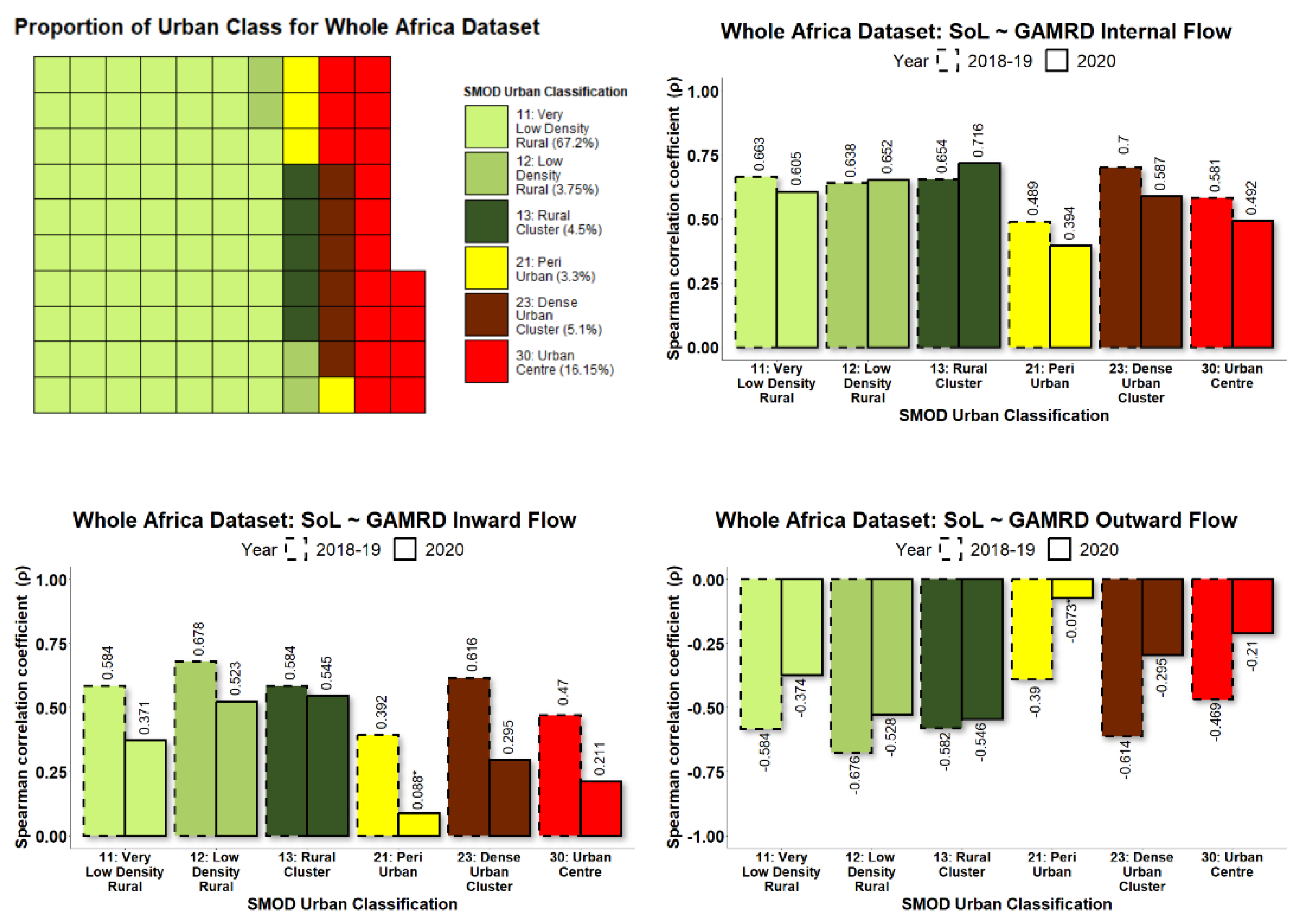
To allow collective analysis over multiple countries, each level 2 administrative unit within each country was categorised according to its degree of urbanisation. By grouping administrative units in this manner, it was possible to demonstrate how NTL and GAMRD correlations vary according to the degree of urbanisation, such as highly populated urban areas vs. sparsely populated rural areas. The GHS Settlement Model (GHS-SMOD) raster provides a classification raster of global coverage that gives for every 1 km² raster pixel a value corresponding to one of eight possible rural/urban classifications (Florczyk et al., 2019) [41] as illustrated in Figure 3.

As the GHS-SMOD raster provides rural/urban classifications at the 1 km² pixel level, an aggregation procedure is required to determine the “overall” degree of urbanisation of each level 2 administrative unit. An R-Script (R v4.0.3) was created for this purpose and took as input: the GHS-SMOD raster as provided by the GHSL-SMOD Project (Florczyk et al., 2019) [41], the 2020 Population Raster as provided by WorldPop (WorldPop-School of Geography and Environmental Science, University of Southampton; Department of Geography and Geosciences, University of Louisville; Departement de Geographie, Universite de Namur; and the Center for International Earth Science Information, n.d.) [42] and the level 2 administrative unit shapefiles for the country of interest. The GHS-SMOD raster was extracted into eight separate rasters for each rural/urban classification and converted to binary format (i.e., 0.1). The WorldPop population raster was then multiplied for each of the eight binary rural/urban classification rasters. The resultant product rasters therefore contained the population count in each rural/urban classification, with the corresponding final level 2 administrative unit values obtained through summation via Zonal Statistics. The eight rural/urban classifications were combined into 3 groups: Group 1 (Classes 10, 11, 12, 13), Group 2 (Classes 21, 22, 23), and Group 3 (Class 30). The final classification was then determined via a nested hierarchy and majority approach whereby each unit was assigned to: Group 1 if Group 1 > 50% total country population, Group 2 if Group 1 < 50% and Group 3 < 50% total country population, or Group 3 if Group 3 > 50% total country population. Within the highest group, the individual highest classification value provided the final rural/urban classification for each administrative unit. A simplified illustration of the procedure using Kenya as an example is shown in Figure 4.

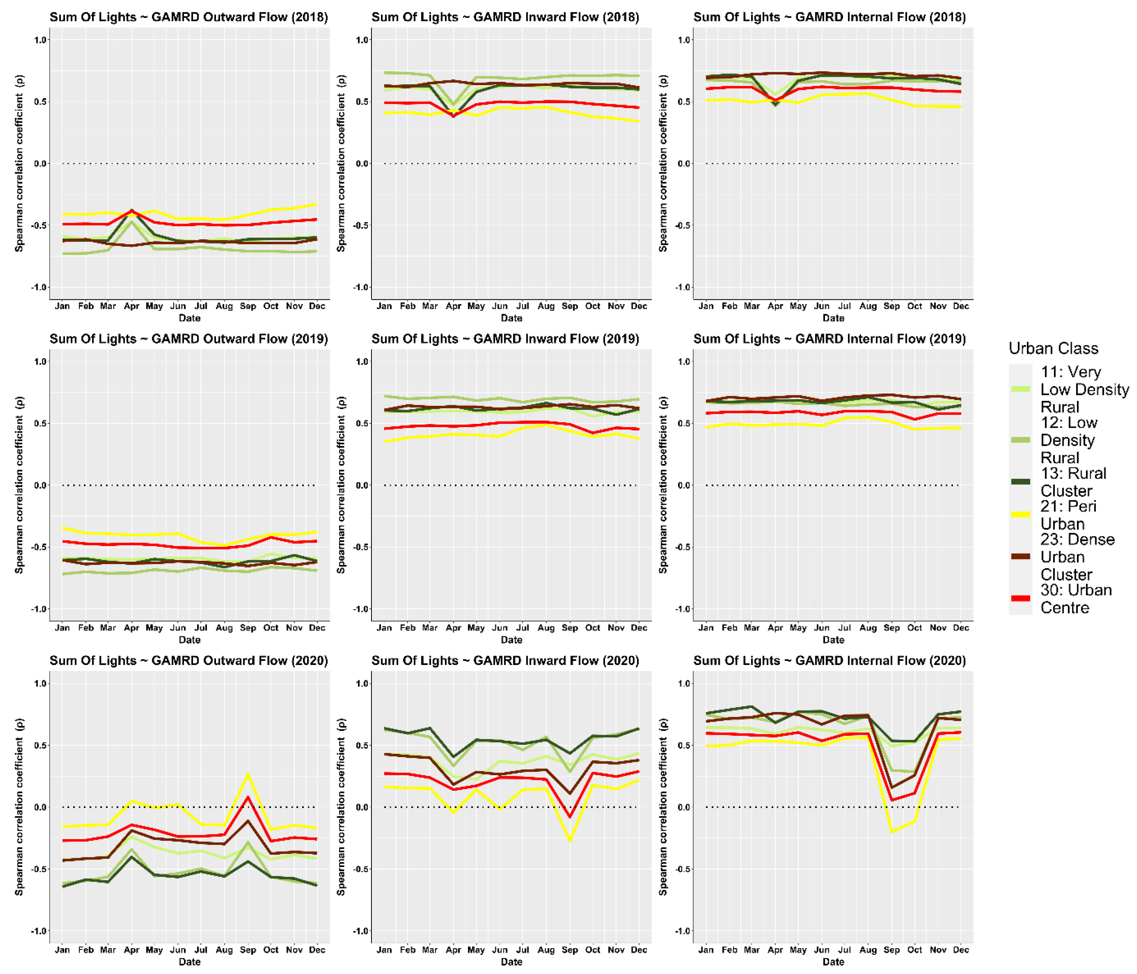
For each administrative unit during the study period 2018–2019 and 2020, NTL data were used to calculate the SoL value per month, while the GAMRD data provided the anonymized and aggregated flows per month. To determine the relationship between GAMRD and NTL data, their monthly values were used as input for a correlation test using the Spearman’s product-moment correlation coefficient (ρ) and its corresponding p-value. By grouping administrative units together according to the rural/urban classification, a high sample size was available for the correlation tests.

Furthermore, we examined the relationship between GAMRD and NTL data in a Gaussian Regression model-based framework to understand the amount of variation in the GAMRD data that could be explained by the NTL data. Both variables were log-transformed to improve the relationship between them and to improve normality. Two models were fitted: (i) a full model that includes NTL and degree of urbanisation as covariates and also accounts for temporal correlation and random variation between countries, and (ii) a reduced model that includes NTL as the only covariate. The reduced model was fitted in a frequentist framework while the full model was fitted in a Bayesian framework using the INLA package in R (Lindgren and Rue, 2015) [43]. The predictive ability of both models was evaluated using a hold-out cross-validation exercise in which we used 80% of the data for model fitting and 20% for validation. The Pearson’s correlation coefficient and the R-squared statistic were then computed using the observed and predicted values. Both the full and reduced models were fitted for each GAMRD-based flow metric (i.e., internal flow, inward flow, and outward flow) separately.

3. Results

3.1. Correlation over Combined Countries

To gain a broad overview of how the NTL SoL values correlate with the three GAMRD flow metrics, all twelve selected African countries were included for the two time periods (i.e., 2018–2019 and 2020). Correlation strength definitions based on the Spearman’s correlation coefficient (ρ) were taken from Akoglu (Akoglu, 2018) [44]. These are ρ (0.1–0.3) = weak correlation, ρ (0.4–0.6) = moderate correlation, and ρ (0.7–0.9) = strong correlation. An example of a typical correlation plot of NTL SoL radiance values ~ GAMRD Inward Flows is shown in Figure 5.

The GAMRD Internal Flow metric for 2018–2019 showed moderate to strong positive correlations in the rural group (11, 12, 13 in Figure 3) and dense-urban class (23 in Figure 3), with weak to moderate correlations in the urban (30 in Figure 3) and peri-urban (21 in Figure 3) classes. For 2020, the correlations were marginally higher in the rural group (11, 12, 13 in Figure 3) and marginally lower in the urban group (21, 23, 30 in Figure 3).

The GAMRD Inward Flow metric for 2018–2019 showed moderate positive correlations in the rural group (11, 12, 13 in Figure 3) and dense-urban class (23 in Figure 3) with weak to moderate correlations in the urban (30 in Figure 3) and peri-urban (21 in Figure 3) classes. For 2020, the correlations were considerably lower in the very-low-density rural (11 in Figure 3) class, marginally less in the rural (12, 13 in Figure 3) group and considerably less in the urban group (21, 23, 30 in Figure 3).

The GAMRD Outward Flow metric for 2018–2019 showed moderate negative correlations in the rural group (11, 12, 13 in Figure 3) and dense-urban (23 in Figure 3) class with weak to moderate correlations in the urban (30 in Figure 3) and peri-urban (21 in Figure 3) classes. For 2020, the correlations were considerably less in the very-low-density rural (11 in Figure 3) class, marginally less in the rural group (12, 13 in Figure 3) and considerably less in the urban group (21, 23, 30 in Figure 3). The Spearman’s correlation coefficients for each rural/urban classification were placed on a bar chart with the relative proportions of each rural/urban classification included for reference as shown in Figure 6.

The results indicated that the rural groups (11, 12, 13 in Figure 3) and dense-urban class (23 in Figure 3) have the highest correlation between the NTL SoL radiance values and GAMRD flow metrics, with the urban group (21, 30 in Figure 3) having the lowest correlations. The differences in correlations between the two time periods were considerable, with 2020 having far smaller correlations coefficients across almost all rural/urban classifications compared to those of 2018–2019.

Using the Gaussian regression model for each time period (i.e., 2018–2019 and 2020), significant positive relationships were observed between the GAMRD flow metrics and NTL SoL radiance values for both internal and inward flows, and significant negative relationships for outward flows. Moreover, significant differences were found between the “urban centre” class and all other rural/urban classifications. The fitted full models showed good predictive power based on the cross-validation exercise results which are shown in

Table 2. Out-of-sample validation NTL-GAMRD statistics based on hold-out cross-validation exercise.

Year	GAMRD Metric	Correlation		R2
		Full Model	Reduced Model	Full Model	Reduced Model
2018–2019	Internal	0.54	0.31	0.29	0.09
	Inward	0.53	0.28	0.28	0.08
	Outward	0.52	0.28	0.27	0.08
2020	Internal	0.48	0.21	0.23	0.04
	Inward	0.51	0.20	0.26	0.04
	Outward	0.47	0.19	0.23	0.04

. For 2018–2019, the out-of-sample R² values of the fitted models were 0.29, 0.28, and 0.27 for the internal, inward, and outward flows, while the corresponding correlations were 0.54, 0.53, and 0.52, respectively. This means that models were able to explain at least 27% of the total variation in the GAMRD flows using NTL SoL as a covariate, whilst adjusting for the other sources of variation in the data. However, with the reduced model, this predictive power reduces to at most 9%, highlighting the importance of accounting for the degree of urbanisation and other sources of variation in the data in the analysis. For 2020, similar results were obtained, although the predictive powers of both the full models (≤26%) and the reduced models (4%) were lower. This can be explained by the fact that while NTL SoL radiance values remained relatively stable throughout all the years (2018, 2019, and 2020), the GAMRD flows significantly decreased.

3.2. Annual Correlation Variation

To gain a deeper insight into why the correlation coefficients for NTL-GAMRD were so different between the two time periods of 2018/19 and 2020, the data were split monthly to analyse any change in correlation during the year, as illustrated in Figure 7. During 2018, the Spearman’s correlation coefficient (ρ) remained relatively stable throughout most of the year for all three GAMRD flow metrics except during April, when the values decreased substantially for the rural group (11, 12, 13 in Figure 3) and “urban centre” class (30 in Figure 3) and increased slightly for the “peri-urban” and “dense urban cluster” classes. During 2019, the Spearman’s correlation coefficient (ρ) remained relatively stable throughout the year across all the rural/urban classifications with the only noticeable perturbation in values during October. During 2020, two large perturbations in the Spearman’s correlation coefficient (ρ) were observed centred around the months of April and September.

3.3. Sum of Lights and GAMRD Annual Value Variation

To determine the possible source of the inter-annual variation of the correlation, the NTL SoL radiance and GAMRD flow totals were analysed separately across each year of 2018, 2019, and 2020. For each year, a combined NTL SoL metric was calculated by grouping all administrative units according to their degree of urbanisation across all countries and then summing the corresponding NTL SoL radiance values for each month, as shown in Figure 8. Whilst the individual values themselves were not analysed, the degree to which this metric varied through the year may highlight months of particularly high variance of the NTL SoL radiance. The variation of the combined NTL SoL metric was most noticeable within the administrative units classified as “urban centres” (30 in Figure 3), whilst for all other rural/urban classifications, the metric was relatively stable throughout all the years 2018, 2019, and 2020.

Similarly, for each of the three GAMRD flow metrics (i.e., internal flow, inward flow, and outward flow), administrative units were grouped according to their degree of urbanisation across all countries, and the corresponding flow values for each month were summed together as shown in Figure 9. As with the combined NTL SoL metric, the total flow values were not directly analysed, but rather their variation throughout the year was used as an indicator of periods of potentially unusual human mobility. During 2018 and 2019, the GAMRD flow totals remained relatively stable for all the rural/urban classifications except the “urban centre” class (30 in Figure 3). During 2020, the “urban centre” class (30 in Figure 3) showed drastic variations across a large range for most months, with two particularly large shifts in April and September, whilst the remaining rural/urban classes remained relatively stable throughout the year.

3.4. Correlation over Country Groups

According to the United Nations Geoscheme for Africa, the twelve study countries were separated to four cardinal groups (north, south, east, and west) and the NTL-GAMRD correlation analysis was repeated as illustrated in Figure A1, Figure A2, Figure A3 and Figure A4 in Appendix A. The Northern Africa group had a high degree of urbanisation with 37.43% of administrative units classified as “urban centres” (30 in Figure 3). Correlation results were generally higher within the rural group (11, 12, 13 in Figure 3) for both the 2018–2019 and 2020 time periods, with correlations for most classes noticeably lower for 2020 than for 2018–2019. The Eastern Africa group had a high degree of rural presence with 66.47% of administrative units classified as “very low density rural” (11 in Figure 3). Correlation results were highest within the rural group (11, 12, 13 in Figure 3) and “urban centres” (30 in Figure 3) for both the 2018–2019 and 2020 time periods, with correlations for most classes noticeably lower for 2020 than for 2018–2019. Correlations for 2020 were comparable with correlations for 2018–2019 across most classes with both positive and negative variance. The Southern Africa group had a balanced rural/urban proportion with neither urban nor rural classifications dominating the administrative units. Correlation results were highest within the rural group (12, 13 in Figure 3) and urban group (23, 30 in Figure 3) for both the 2018–2019 and 2020 time periods, with correlations for 2020 considerably lower than correlations for 2018–2019 for all classes. The Western Africa group had a high degree of rural presence with 82.58% of administrative units classified as “very low density rural” (11 in Figure 3). Correlation results were highest within the urban group (21, 23, 30 in Figure 3) for both the 2018–2019 and 2020 time periods, with correlations for 2020 noticeably lower than correlations for 2018–2019 for most classes. Correlations for 2020 were comparable with correlations for 2018–2019 across most classes with both positive and negative variance.

4. Discussion

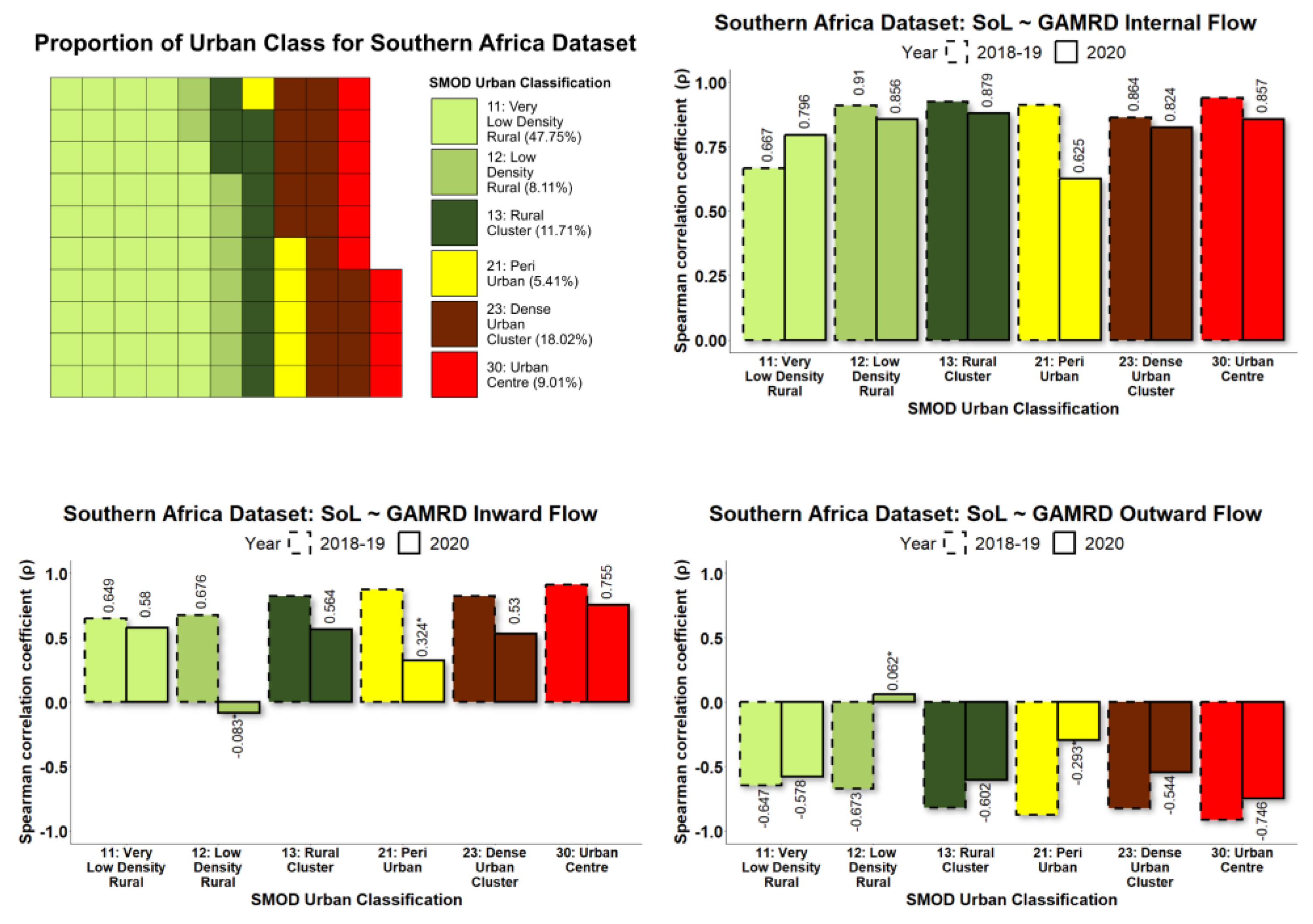
NTL has been widely used for population spatial distribution mapping, and a strong correlation between NTL and GAMRD data has been demonstrated in previous studies (Dickinson et al., 2020) [30]; however, the variation of this relationship according to the degree of urbanisation was previously unexplored. The longitudinal Google Aggregated Mobility Research Dataset (GAMRD) and the VIIR NTL data for Africa in 2018–2020, according to the degree of urbanisation, provide a good opportunity to improve our understanding of the value of NTL data for assessing human mobility and the associated changes in population presence in low- and middle-income countries. The diversity of the study’s countries in different regions does ensure that this study contains wide variance in socioeconomic, geographic, and demographic contexts. Our study, conducted from 2019–2021, has demonstrated the high variability in correlations between administrative-unit-level NTL radiance values and GAMRD flow metrics across a broad geographic range and within different rural/urban classifications. Administrative units classified as rural and semi-rural were shown to have on average the highest NTL-GAMRD correlation whilst administrative units classified as “urban centres” had the lowest (not including the peri-urban class, which had several low p-values). This is likely due to the saturation and greater stability of lighting and NTL brightness values within urban centres/areas. Indeed, large urban centres/areas in Sub-Saharan Africa and elsewhere tend to be more consistently lit throughout the year and are often bright enough in their core to saturate NTL brightness values (Zhao et al., 2019) [45]. This means that changes in brightness due to human mobility and the associated population presence and density changes are less likely to occur in urban centres/areas than in small towns/rural and peri-urban areas, where population arrivals may lead to an increase in brightness due to electric lighting or fires in residential areas (Bharti et al., 2011) [12].

What was most noticeable in the study was the significant difference in correlation strength between the two time periods of 2018–2019 and 2020. Correlations across most rural/urban classifications and particularly “urban centres” were considerably lower in 2020 than in 2018–2019. Whilst the variation of the NTL SoL radiance values across all urban classes remained relatively stable throughout the year, the GHL flow metrics referring to 2020 showed that the corresponding flow values were far more erratic than those in 2018–2019, with the months of April and September being most prominent in their deviation, creating a consequential effect for the NTL-GAMRD correlations during these months. These changes might be attributed to the implementation of lockdown measures during the COVID-19 pandemic, with the first wave in March–April (Haider et al., 2020) [46] and the second wave in September–October (Kuehn, 2021) [47]. This has implications for the reliability of NTL data as a proxy for human mobility during periods of unusual human activity, such as lockdown periods. In addition, NTL data have several drawbacks such as delayed access to real-time data, low light detection thresholds, and the requirement for additional postprocessing; however, these are expected to continue to be addressed as the technology further develops and novel data sources become available (Zhao et al., 2019) [45].

In addition, we only found one similar study conducted by Dickinson et al., 2020 [30]. Based on linear regression and random forest models, they used Google’s human mobility data in 2016 to predict VIIRS satellite imagery and then assessed how accurately this simulated global NTL imagery could be used to predict GDP across regions in 2015–2016. They demonstrated that the relationship between human mobility and VIIRS NTL was nonlinear and varied considerably around the globe. The differences across regions were made clear by the improvement in the model performance when modelling each region independently rather than constructing a single global model. Our study further measured the degree to which this relationship varied across locations with different levels of urbanisation and development in 2018–2020. However, we found that compared with urban settings, there was a higher association between NTL data and mobility changes in rural and peri-urban areas. In addition, a reduced NTL-GAMRD correlation strength in 2020 was observed, especially in urban settings, most probably because of the monthly NTL SoL radiance values remaining relatively similar in 2018–2019 and 2020 but the human mobility significantly decreasing in 2020 with respect to the previous considered period. Our study provides new insights about changes in mobility and NTL as well as their association across settings during a global crisis such as the pandemic.

Furthermore, it is important to highlight that GAMRD data present several limitations and potential biases as well. Indeed, such data are limited to mobile internet coverage and smartphone users who have opted into Google’s Location History feature, which is off by default, and thus, they may not be representative of the population as a whole. Similarly, their representativeness may vary by location and be particularly low in rural areas characterised by low population densities. Additionally, GAMRD data are still likely to be biased towards educated males living in urban areas (Lai, zu Erbach-Schoenberg et al., 2019) [25]. Moreover, comparisons across rather than within locations are only descriptive, since these regions can differ in substantial ways. Another primary drawback of GAMRD data is the difficulty of obtaining them due to the restrictive data sharing policies implemented to protect individual privacy and GAMRD data being subject to differential privacy algorithms designed to protect user’s anonymity, which obscure fine details. However, considering potential biases of representativeness among populations across regions, it is important to include subnational and up-to-date statistics on smart-device ownership and internet penetration in future research where possible. Mobile phone subscribers and smartphone adoption are expected to continue growing in low- and middle-income countries, and surveys for measuring mobile phone/smartphone penetration and social media coverage may be necessary to obtain more precise metrics for each country and subnational region (e.g., administrative unit level 1 or 2). In addition, considering the potential biases of representativeness among populations, rather than grouping countries together, it may be of interest to analyse each country separately to avoid generalisations in the future.

5. Conclusions

Following the global COVID-19 pandemic and the consequent restrictions on human mobility, importance has risen dramatically for datasets that can successfully explore short-term and intra-annual human mobility and assess the associated population presence and density changes. With several proxies available, it is useful to understand the limitations and accuracy of each dataset that can be used for mobility research, which motivates the current study. Results have indicated that VIIRS NTL data may be best-suited for the analysis of human mobility within more rural areas and that during periods of unusual human activity (such as the lockdown periods in 2020), VIIRS NTL data may not provide the necessary spatial resolution for detailed study. In addition, as the NTL-GAMRD correlation was found to be potentially weaker in “urban centres” areas, this highlights the importance of integrating additional geospatial datasets that are able to capture different scales of variation into a larger multivariate model, instead of our current simple modelling framework.

As refinements in NTL technology become available and new datasets are released with higher spatial resolution and enhanced postprocessing, it is hoped that these limitations may be overcome. Despite the demonstrated efficacy of the GAMRD in “urban centres” areas and during lockdown periods, with NTL data continuing to be publicly available with wide geographic coverage, its use can remain important as a proxy of human mobility and the associated population presence and density changes until alternative datasets, such as mobile phone locations, can be more easily accessed by the scientific and operational communities.

References

1. Grenfell, B.T.; Bjørnstad, O.N.; Kappey, J. Travelling waves and spatial hierarchies in measles epidemics. Nature 2001, 414, 716–723. [Google Scholar] [CrossRef]
2. Wesolowski, A.; Eagle, N.; Tatem, A.J.; Smith, D.L.; Noor, A.M.; Snow, R.W.; Buckee, C.O. Quantifying the Impact of Human Mobility on Malaria. Science 2012, 338, 267–270. [Google Scholar] [CrossRef]
3. Wesolowski, A.; Metcalf, C.J.E.; Eagle, N.; Kombich, J.; Grenfell, B.T.; Bjørnstad, O.N.; Lessler, J.; Tatem, A.J.; Buckee, C.O. Quantifying seasonal population fluxes driving rubella transmission dynamics using mobile phone data. Proc. Natl. Acad. Sci. USA 2015, 112, 11114–11119. [Google Scholar] [CrossRef]
4. Wesolowski, A.; Qureshi, T.; Boni, M.F.; Sundsøy, P.R.; Johansson, M.A.; Rasheed, S.B.; Engø-Monsen, K.; Buckee, C.O. Impact of human mobility on the emergence of dengue epidemics in Pakistan. Proc. Natl. Acad. Sci. USA 2015, 112, 11887–11892. [Google Scholar] [CrossRef] [PubMed]
5. Steele, J.E.; Pezzulo, C.; Albert, M.; Brooks, C.J.; zu Erbach-Schoenberg, E.; O’Connor, S.B.; Sundsøy, P.R.; Engø-Monsen, K.; Nilsen, K.; Graupe, B.; et al. Mobility and phone call behavior explain patterns in poverty at high-resolution across multiple settings. Humanit. Soc. Sci. Commun. 2021, 8, 288. [Google Scholar] [CrossRef]
6. Strano, E.; Viana, M.P.; Sorichetta, A.; Tatem, A.J. Mapping road network communities for guiding disease surveillance and control strategies. Sci. Rep. 2018, 8, 4744. [Google Scholar] [CrossRef]
7. Lai, S.; Sorichetta, A.; Steele, J.; Ruktanonchai, C.W.; Cunningham, A.D.; Rogers, G.; Koper, P.; Woods, D.; Bondarenko, M.; Ruktanonchai, N.W.; et al. Global holiday datasets for understanding seasonal human mobility and population dynamics. Sci. Data 2022, 9, 17. [Google Scholar] [CrossRef]
8. Mao, L.; Wu, X.; Huang, Z.; Tatem, A.J. Modeling monthly flows of global air travel passengers: An open-access data resource. J. Transp. Geogr. 2015, 48, 52–60. [Google Scholar] [CrossRef]
9. Song, B.; Yan, X.-Y.; Tan, S.; Sai, B.; Lai, S.; Yu, H.; Ou, C.; Lu, X. Human mobility models reveal the underlying mechanism of seasonal movements across China. Int. J. Mod. Phys. C 2021, 33, 2250054. [Google Scholar] [CrossRef]
10. Woods, D.; Cunningham, A.; Utazi, C.E.; Bondarenko, M.; Shengjie, L.; Rogers, G.E.; Koper, P.; Ruktanonchai, C.W.; zu Erbach-Schoenberg, E.; Tatem, A.J.; et al. Exploring methods for mapping seasonal population changes using mobile phone data. Humanit. Soc. Sci. Commun. 2022, 9, 247. [Google Scholar] [CrossRef]
11. Bharti, N.; Tatem, A.J. Fluctuations in anthropogenic nighttime lights from satellite imagery for five cities in Niger and Nigeria. Sci. Data 2018, 5, 180256. [Google Scholar] [CrossRef] [PubMed]
12. Bharti, N.; Tatem, A.J.; Ferrari, M.J.; Grais, R.F.; Djibo, A.; Grenfell, B.T. Explaining seasonal fluctuations of measles in Niger using nighttime lights imagery. Science 2011, 334, 1424–1427. [Google Scholar] [CrossRef] [PubMed]
13. Bustos, M.F.A. Population, Demography and Nighttime Lights an Examination of the Effects of Population Decline on Settlement Patterns in Europe. 2015. Available online: http://www.cfe.lu.se (accessed on 28 July 2023).
14. Elvidge, C.D.; Baugh, K.E.; Anderson, S.J.; Sutton, P.C.; Ghosh, T. The Night Light Development Index (NLDI): A spatially explicit measure of human development from satellite data. Soc. Geogr. 2012, 7, 23–35. [Google Scholar] [CrossRef]
15. Doll, C.N.H.; Muller, J.-P.; Elvidge, C.D. Night-time imagery as a tool for global mapping of socioeconomic parameters and greenhouse gas emissions. AMBIO A J. Hum. Environ. 2000, 29, 157–162. [Google Scholar] [CrossRef]
16. Ebener, S.; Murray, C.; Tandon, A.; Elvidge, C.C. From wealth to health: Modelling the distribution of income per capita at the sub-national level using night-time light imagery. Int. J. Health Geogr. 2005, 4, 5. [Google Scholar] [CrossRef]
17. Elvidge, C.D.; Baugh, K.E.; Zhizhin, M.; Hsu, F.-C. Why VIIRS data are superior to DMSP for mapping nighttime lights. Proc. Asia-Pac. Adv. Netw. 2013, 35, 62. [Google Scholar] [CrossRef]
18. Lai, S.; Farnham, A.; Ruktanonchai, N.W.; Tatem, A.J. Measuring mobility, disease connectivity and individual risk: A review of using mobile phone data and mHealth for travel medicine. J. Travel Med. 2019, 26, taz019. [Google Scholar] [CrossRef]
19. Chen, X. Nighttime Lights and Population Migration: Revisiting Classic Demographic Perspectives with an Analysis of Recent European Data. Remote Sens. 2020, 12, 169. [Google Scholar] [CrossRef]
20. Stathakis, D.; Baltas, P. Seasonal population estimates based on night-time lights. Comput. Environ. Urban Syst. 2018, 68, 133–141. [Google Scholar] [CrossRef]
21. Tselios, V.; Stathakis, D. Exploring regional and urban clusters and patterns in Europe using satellite observed lighting. Environ. Plan. B Urban Anal. City Sci. 2020, 47, 553–568. [Google Scholar] [CrossRef]
22. Xu, G.; Xiu, T.; Li, X.; Liang, X.; Jiao, L. Lockdown induced night-time light dynamics during the COVID-19 epidemic in global megacities. Int. J. Appl. Earth Obs. Geoinf. 2021, 102, 102421. [Google Scholar] [CrossRef] [PubMed]
23. Lu, X.; Wrathall, D.J.; Sundsøy, P.R.; Nadiruzzaman; Wetter, E.; Iqbal, A.; Qureshi, T.; Tatem, A.J.; Canright, G.S.; Engø-Monsen, K.; et al. Detecting climate adaptation with mobile network data in Bangladesh: Anomalies in communication, mobility and consumption patterns during cyclone Mahasen. Clim. Change 2016, 138, 505–519. [Google Scholar] [CrossRef]
24. Montoya-Rincon, J.P.; Azad, S.; Pokhrel, R.; Ghandehari, M.; Jensen, M.P.; Gonzalez, J.E. On the Use of Satellite Nightlights for Power Outages Prediction. IEEE Access 2022, 10, 16729–16739. [Google Scholar] [CrossRef]
25. Lai, S.; zu Erbach-Schoenberg, E.; Pezzulo, C.; Ruktanonchai, N.W.; Sorichetta, A.; Steele, J.; Li, T.; Dooley, C.A.; Tatem, A.J. Exploring the use of mobile phone data for national migration statistics. Palgrave Commun. 2019, 5, 34. [Google Scholar] [CrossRef]
26. Ruktanonchai, N.W.; Ruktanonchai, C.W.; Floyd, J.; Tatem, A.J. Using Google Location History data to quantify fine-scale human mobility. Int. J. Health Geogr. 2018, 17, 28. [Google Scholar] [CrossRef] [PubMed]
27. Bengtsson, L.; Lu, X.; Thorson, A.; Garfield, R.; von Schreeb, J. Improved response to disasters and outbreaks by tracking population movements with mobile phone network data: A post-earthquake geospatial study in haiti. PLoS Med. 2011, 8, e1001083. [Google Scholar] [CrossRef]
28. Buckee, C.O.; Wesolowski, A.; Eagle, N.N.; Hansen, E.; Snow, R.W. Mobile phones and malaria: Modeling human and parasite travel. Travel Med. Infect. Dis. 2013, 11, 15–22. [Google Scholar] [CrossRef]
29. Ruktanonchai, N.W.; DeLeenheer, P.; Tatem, A.J.; Alegana, V.A.; Caughlin, T.T.; Zu Erbach-Schoenberg, E.; Lourenço, C.; Ruktanonchai, C.W.; Smith, D.L. Identifying Malaria Transmission Foci for Elimination Using Human Mobility Data. PLoS Comput. Biol. 2016, 12, e1004846. [Google Scholar] [CrossRef]
30. Dickinson, B.; Ghoshal, G.; Dotiwalla, X.; Sadilek, A.; Kautz, H. Inferring Nighttime Satellite Imagery from Human Mobility. In Proceedings of the AAAI Conference on Artificial Intelligence, New York, NY, USA, 7–12 February 2020; Volume 34, pp. 394–402. [Google Scholar] [CrossRef]
31. Bassolas, A.; Barbosa-Filho, H.; Dickinson, B.; Dotiwalla, X.; Eastham, P.; Gallotti, R.; Ghoshal, G.; Gipson, B.; Hazarie, S.A.; Kautz, H.; et al. Hierarchical organization of urban mobility and its connection with city livability. Nat. Commun. 2019, 10, 4817. [Google Scholar] [CrossRef]
32. Wilson, R.J.; Zhang, C.Y.; Lam, W.; Desfontaines, D.; Simmons-Marengo, D.; Gipson, B. Differentially Private SQL with Bounded User Contribution. Proc. Priv. Enhancing Technol. 2020, 2020, 230–250. [Google Scholar] [CrossRef]
33. Google. How Google Anonymises Data. Retrieved from Google Privacy&Terms. Available online: https://policies.google.com/technologies/anonymization (accessed on 28 July 2023).
34. S2 Geometry. 2018. Available online: http://s2geometry.io/ (accessed on 28 July 2023).
35. Elvidge, C.D.; Baugh, K.; Zhizhin, M.; Hsu, F.C.; Ghosh, T. VIIRS night-time lights. Int. J. Remote Sens. 2017, 38, 5860–5879. [Google Scholar] [CrossRef]
36. Mills, S.; Weiss, S.; Liang, C. VIIRS day/night band (DNB) stray light characterization and correction. In Earth Observing Systems XVIII; SPIE: Bellingham, WA, USA, 2013; Volume 8866, p. 88661P. [Google Scholar]
37. Li, X.; Xu, H.; Chen, X.; Li, C. Potential of NPP-VIIRS Nighttime Light Imagery for Modeling the Regional Economy of China. Remote Sens. 2013, 5, 3057–3081. [Google Scholar] [CrossRef]
38. Wang, R.; Wan, B.; Guo, Q.; Hu, M.; Zhou, S. Mapping Regional Urban Extent Using NPP-VIIRS DNB and MODIS NDVI Data. Remote Sens. 2017, 9, 862. [Google Scholar] [CrossRef]
39. Warmerdam, F. The geospatial data abstraction library. In Open Source Approaches in Spatial Data Handling; Springer: Berlin, Germany, 2008; pp. 87–104. [Google Scholar]
40. UN Statistics Division. Methodology: Standard Country or Area Codes for Statistical Use (M49); Questions & Answers; UN Statistics Division: New York, NY, USA, 2022. [Google Scholar]
41. Florczyk, A.J.; Corbane, C.; Ehrlich, D.; Freire, S.; Kemper, T.; Maffenini, L.; Melchiorri, M.; Pesaresi, M.; Politis, P.; Schiavina, M.; et al. GHSL Data Package 2019; JRC Technical Report; European Commission, Publications Office of the European Union: Luxembourg, 2019.
42. WorldPop—School of Geography and Environmental Science, University of Southampton; Department of Geography and Geosciences, University of Louisville; Departement de Geographie, Universite de Namur and Center for International Earth Science Information, Global High Resolution Population Denominators Project. 2018. Available online: https://hub.worldpop.org/geodata/summary?id=24767 (accessed on 28 July 2023). [CrossRef]
43. Lindgren, F.; Rue, H. Bayesian Spatial Modelling with R-INLA. J. Stat. Softw. 2015, 63, 1–25. [Google Scholar] [CrossRef]
44. Akoglu, H. User’s guide to correlation coefficients. Turk. J. Emerg. Med. 2018, 18, 91–93. [Google Scholar] [CrossRef] [PubMed]
45. Zhao, N.; Samson, E.L.; Liu, Y. Population bias in nighttime lights imagery. Remote Sens. Lett. 2019, 10, 913–921. [Google Scholar] [CrossRef]
46. Haider, N.; Osman, A.Y.; Gadzekpo, A.; O Akipede, G.; Asogun, D.; Ansumana, R.; Lessells, R.J.; Khan, P.; Hamid, M.M.A.; Yeboah-Manu, D.; et al. Lockdown measures in response to COVID-19 in nine sub-Saharan African countries. BMJ Glob. Health 2020, 5, e003319. [Google Scholar] [CrossRef]
47. Kuehn, B.M. Africa Succeeded Against COVID-19′s First Wave, but the Second Wave Brings New Challenges. Jama 2021, 325, 327–328. [Google Scholar] [CrossRef]
Figure 1. The 12 African countries selected for the current study and grouped according to the United Nations Geoscheme for Africa.
Remotesensing 15 04252 g001
Figure 2. Workflow for extracting and postprocessing VIIRS night-time lights imagery.
Remotesensing 15 04252 g002
Figure 3. The GHS Settlement Model (GHS-SMOD) rural/urban classification definitions.
Remotesensing 15 04252 g003
Figure 4. Visual overview of the process to determine urban classification at the administrative unit level: The GHSL-SMOD raster (A) is multiplied by the corresponding population raster (B) which is ran through zonal statistics to obtain the majority urban classification for the admin units of each country’s level 2 shapefile (C).
Remotesensing 15 04252 g004
Figure 5. A sample of a correlation plot between the NTL SoL radiance values and GAMRD Inward Flows for the low-density rural class (12 in Figure 3) across all twelve selected African countries during the 2018–2019 period.
Remotesensing 15 04252 g005
Figure 6. The proportion of rural/urban classifications for all level 2 administrative units within the 12 selected Africa countries (top left). The Spearman’s correlation coefficients for each rural/urban classification for the NTL SoL radiance values and GLH flow metrics. All values p < 0.0001 except those indicated by an asterisk *.
Remotesensing 15 04252 g006
Figure 7. Spearman’s correlation coefficient variation per month between NTL SoL radiance values and GLH flow metrics for the 12 selected Africa countries over the years 2018, 2019, and 2020.
Remotesensing 15 04252 g007
Figure 8. The combined NTL SoL metric for all administrative units in each month in 2018, 2019, and 2020 across all twelve selected African countries.
Remotesensing 15 04252 g008
Figure 9. The total GLH flow parameters summed over all administrative units and grouped according to urban classification.
Remotesensing 15 04252 g009