

Slip Estimation Using Variation Data of Strain of the Chassis of Lunar Rovers Traveling on Loose Soil
1
Department of Machinery and Control Systems, College of Systems Engineering and Science, Shibaura Institute of Technology, Saitama 337-8570, Japan
2
Systems Engineering and Science, Graduate School of Engineering and Science, Shibaura Institute of Technology, Saitama 337-8570, Japan
*
Author to whom correspondence should be addressed.
Remote Sens. 2023, 15(17), 4270; https://doi.org/10.3390/rs15174270
Submission received: 21 June 2023
/
Revised: 22 August 2023
/
Accepted: 26 August 2023
/
Published: 30 August 2023
(This article belongs to the Special Issue Future of Lunar Exploration)
Abstract
:The surface of the Moon and planets have been covered with loose soil called regolith, and there is a risk that the rovers may stack, so it is necessary for them to recognize the traveling state such as its posture, slip behavior, and sinkage. There are several methods for recognizing the traveling state such as a system using cameras and Lidar, and they are used in real exploration missions like Mars Exploration Rovers of NASA/JPL. When a rover travels and travels across loose soil with steep slopes like a side wall of a crater on the lunar surface, the rover has side slipping. It means that its behavior makes the rover slip down to the valley direction. Even if this detection uses sensors like a camera and Lidar or other controlling systems like SLAM (Simultaneous Localization and Mapping), it would be too difficult for the rover to avoid slipping down to valley direction, because it is not able to detect the traction or resistance given from ground by individual wheel of the rover, as the traction of individual wheel of the rover is not clear. This means that the movement of the rover appeared by integrating the traction of all wheels mounted on the rover. Even if the localization by sensors is carried out, the location would be the location after slipping down. This is because when traveling on unstable ground, the driving force of each individual wheel cannot be accurately predicted, and the sum of the driving force of all wheels is the motion of the rover, which is detected after the position changes. Therefore, if the rover obtains information on the traction of each wheel, its maneuver to change its posture would work sooner and it would be able to travel more efficiently than in a state without that information. Because the onboard computer of rovers can identify their location and state from the information of the traction of each wheel, they can decide the next work carefully and in detail. From these tasks, we focused on the intrinsic sensation of a biological function like a human body and aimed to develop a system that recognizes the traveling state (slip condition) from the shape deformation of the chassis. In this study, we experimentally verified the relationship between the change in strain, which is the amount of deformation acting on the chassis, and the traveling state while the wheel is traveling. From the experimental results, we confirmed that the strain in the chassis was displaced dynamically and that the strain changed oscillatory while the wheel was traveling. In addition, based on the function of muscle spindles as mechanoreceptors, we discussed two methods of analyzing strain change: nuclear chain fiber analysis and nuclear bag fiber analysis. These analyses mean that the raw data of the strain are updated to detect the characteristic strain elements of a chassis while the wheel is traveling through loose soil. Eventually, the slipping state could be estimated by updating the data of a lot of strain raw data, and it was confirmed that the traveling state could be detected.
1. Introduction
Space development has been actively conducted in order to expand the scope of human activities with the development of science and technology. The demand for landing exploration using a rover has increased. However, it is a dangerous environment for humanity such as extreme temperature, radiation, and thin atmosphere [1]. Therefore, it has been required to use a rover for an unmanned exploration mission. Specifically, planetary rovers will be used to carry equipment for lunar exploration, to search for ice at the poles, or to explore Mars, especially to investigate the existence of life [2,3,4].
On the Moon and planets, there are many slopes such as craters, cliffs, and dunes [5]. These areas are important observation stations because they have exposed crust and eternal darkness, which are of great scientific interest [6,7].
In fact, the Schrödinger basin has been investigated and found to be an important site [8,9]. In fact, the Mars Exploration Rovers have also conducted geological surveys by polishing [4,10].
Furthermore, machine learning approaches for autonomous data analysis have been studied for the Mars Exploration Rovers [11].
Recently, even the far side of the Moon has been explored, as in the case of Chang’E-4 with the Yutu-2 rover [12,13]. However, the surface is covered with fine particles called regolith, which causes the wheels to slip when the rover travels. If the slippage is not restrained, exploration efficiency will decrease because the robot will deviate from the planned target path. In the worst case, the rover becomes stacked, and exploration becomes impossible [14]. Stuck means the wheels are buried in the sand and cannot move. In fact, the Mars Exploration Rover MER (NASA, JPL, 2012) became stuck on Mars and took more than a month to escape [15]. Therefore, if the rover can detect the traveling state (slip condition), it can correct the misalignment of the traveling path and avoid the stuck state. In order to detect the traveling state (slip condition), detection systems based on visual information using cameras loaded on rovers have been studied, such as relative position estimation and traveling ground discrimination [16,17,18,19]. There is a technology called Simultaneous Localization and Mapping (SLAM). SLAM is a technology that performs simultaneous localization and mapping and is used in many automated vehicles [20,21,22,23]. However, there is a risk that the accuracy of detection will be decreased by the effects such as fewer feature points in the image (the term “less feature points” indicates that the surface is covered with sand and is visually the same color as no rocks or stones, and thus no feature points can be detected by cameras or sensors). The system cannot respond to sudden slippage because it cannot detect small changes in slippage. It is possible to improve the tracking of the travel path and prevent stuck states if the rover can recognize the travel state. Therefore, a new system for detecting the traveling state (slip condition) is required. This is especially necessary when a rover travels across loose soil with steep slopes, such as the sidewalls of craters on the Moon. This means that it is controlled by integrating the traction of each wheel. If the rover obtains information on the traction of each wheel, its maneuver to change its posture would work sooner and it would be able to travel more efficiently than in a state without that information. Because the rovers can understand a mechanical state from the information on the traction of each wheel, and they can decide on the next work carefully and in detail. There are some terramechanic models that can be represented by a single wheel placed on loose soil [24,25]. The drawbar pulls or the driving force can be obtained from these models. Since the wheels are buried when traveling on loose ground, it is necessary to consider the amount of burial. In other words, these models are related to the ground contact conditions between the wheels and the ground and then is necessary to calculate the normal and shear stresses to calculate the traction force. In addition, characteristics of the ground (e.g., angle of repose) and the geometry of the wheel are considered. Finally, the traction force is calculated using the slip rate as an input value. These ones need the value of “slip ratio” to calculate this model, and slip ratio is used as input data for these models. Therefore, if the rovers would calculate a driving force from these models on the spot, we need real-time data on the slip ratio. Although the value of slip ratio can be calculated using the displacement of a rover and the rotational angle of wheels, its accuracy depends on the accuracy of a sensing system like SLAM and so on. In addition, it is necessary for these models to know other information like sinkage, some soil factors in detail, and so on, beforehand. These systems would inevitably contain some errors. In practice, rovers sent to a Moon-like planetary body would use terramechanic models with some predictive capabilities. For example, a pre-simulated database from a lot of experiments on Earth may be used. However, it is difficult for rovers to predict accuracy on the spot because a rover would travel on loose soil including high nonlinear. Humans use not only “vision” but also somatosensory perception to recognize their walking condition. Particularly, an intrinsic sensation is one of the somatosensory senses that estimates the body motion and position change from the stimulation of muscles, tendons, and joints [26,27]. In fact, humans receive forces applied to the lower limbs as mechanical stimuli called “tension” and recognize the walking state based on this information. Therefore, we focused on some elements of the intrinsic sensory functions and tried to construct the system to detect the traveling state (slip condition) based on these. This phenomenon of human muscles also occurs in the chassis of a rover. When the rover travels, the force applied to the wheels changes with the ground and traveling state (slip condition). These forces affect the chassis of the rover and change the shape of the chassis. We aim to develop a system that detects this change in the shape of the chassis and recognizes the traveling state (slip condition) based on intrinsic sensory information. Figure 1 shows the outline of the traveling state (slip condition) detection system.
In this study, the relationship between the change in the amount of strain, which is the deformation of a chassis, and the traveling state (slip condition) is confirmed by a traveling experiment in order to develop the system. First, the phenomenon is confirmed by measuring the strain that occurred during traveling experiments with a single wheel. In addition, the analysis method of the strain during traveling is discussed by using the strain at this time. Finally, based on the analyzing method, the effectiveness of this method is confirmed by measuring the change in strain when the traveling state (slip condition) is set in different situations like traveling ground (rigid surface, loose soil) and forced towing force.
This work estimates the driving force and slip state generated from a single wheel, and this estimation can improve the accuracy of estimating the driving force acting on the entire vehicle. It also has the possibility to control the traction generated by each wheel. If the traction and slip acting on a single wheel can be estimated, this is an effective method that can greatly improve the tracking performance of path planning.
In addition, many lunar and Mars exploration missions are planned by various organizations [28,29,30], and multiple rovers will be deployed on the planetary surfaces in the future [31]. In this paper, we discuss the prospect of using the strain information (proposed here) obtained from the chassis of the rovers as a remote sensing technique.
2. Traveling on Loose Soil and the Small Deformation of the Chassis
2.1. About the Wheel of the Rover Traveling on Loose Soil
The movement of a rover is caused by the sum of forces produced by the rotation of each wheel as previously described. The amount of displacement caused by these forces (the sum of the forces of each wheel) is detected and calculated by sensing systems such as SLAM, and then the trajectory of a rover is corrected. The physical model using the attitude of a rover is adapted to the maneuver of a rover, and the order like the rotation of wheels from information calculated by this model is sent on it. In the case of rough terrain like the Martian surface or lunar surface, the interaction model called the “Terramechanis model” is used [32,33,34]. This model can calculate the driving force from slip ratio and amount of sinkage during traveling loose soil as indicated in Figure 2. The slip rate is defined as the ratio of the actual movement of the rover to the ideal movement calculated from the amount of wheel rotation. This model needs to be given some soil parameters to calculate the equation. The parameters are soil coefficient, slip rate, amount of wheel burial, and so on. There are two problems in order to obtain driving force on time and on the spot. First, the rover obtains the value of slip ratio and amount of sinkage on real-time data. For others, the rover must acquire some soil parameters beforehand. The rover cannot obtain accurate data from these problems because it is difficult to obtain these data on the spot in real time. Even if the rover can predict this information beforehand, it is difficult to predict the value of the driving force of each wheel and there is a significant error in acquired and calculated data. It needs to obtain information such as the driving force of “each” wheel to predict a value close to an accuracy data. If these data are given, the rover can be controlled by traction produced by “each” wheel and then travel accurately along the planning path. As mentioned above, some elements are necessary for the driving force prediction using the terramechanics model, but the terramechanics model simply shows the dynamic elements like shearing stress, and normal stress, and it is effective to consider logically (when a wheel travels on loose ground, a wheel is buried in the soil. In other words, a wheel is in contact with the loose soil to a certain area on the wheel surface. In order to represent this, it is effective to use normal stress and shear stress). In addition, if the value of the slip ratio is acquired on the spot, the driving force of each wheel can be calculated using the terramechanics model (in this study, we directly obtain the driving force data using the force sensor as the true value). In the terramechanics model, which indicated the relationship between a wheel and loose soil, two elements, shearing stress, and normal stress, are very important. The equation of driving force Fx is expressed using the normal stress σ, the shearing stress τ, the wheel radius r, and the wheel width b. s represents the slip ratio. θ is the value (angle) used for integration with respect to the stress region. θf and θr represent the inserting angle and the exit angle individually.
The normal stress σ(θ) is divided before and after the maximum occurrence stress angle θm and is expressed by two equations [35]. σmax is the maximum normal stress and n is the soil parameter.
The sharing stress is expressed using the cohesion stress of the soil c, internal friction angle ϕ and kx is the shear deformation module as follows [36]. And the soil deformation jx is indicated in Equation (5) [35].
These elements are dependent on sinkage during the wheel traveling loose soil (in case of traveling the rigid surface, these elements are not considered). When the wheel sinks into loose soil, the surface of the wheel contact with loose soil becomes a curved surface. Moreover, the surface is formed while being destroyed. The movement of this wheel at this time is very complicated and there are many soil grains existing with various vectors of driving direction on detailed points on the wheel’s surface. This means that soil movement and stress distribution under the wheel is very complicated. The actual movement of each wheel of the rover can be estimated by integrating these complicated forces. If the information of this integrating force at each wheel can be obtained on the spot at the time, the movement prediction function of the rover will be able to improve. When the wheel of the rover travels loose soil, the chassis of the wheels gets influenced by dynamic force. The chassis is connected to the wheel and body of the rover. This means that the construction of these chassis undergoes small deformation by dynamic forces while traveling on loose soil. These dynamic forces caused by traveling on loose soil are not the same as the state where the wheel is traveling on a rigid surface like artificially maintained roads as mentioned above. Therefore, this study focuses on the relationship between the small deformation that occurs on the chassis of the wheel sinking into the soil and the slip ratio. Then, the estimation method of the slip ratio using the data of these small deformations in the chassis is proposed.
2.2. The Small Deformation That Occurs in the Chassis of the Wheel
Figure 3 shows the traveling state of the wheel on a rigid surface and loose soil. In the case of the traveling state on a rigid surface (Figure 3a), the contact range between the wheel and this surface is grounded along a “line”. At the beginning of traveling, the static friction changes to the dynamic friction with slippage, and then the wheel starts moving. The wheel moves firster than the chassis and the body. In this case, a moment is generated in the chassis connected to the wheel axle, and the chassis deflects. The chassis then tries to recover the deflection. This process is repeated. This process continues while the wheel is moving and slipping on the loose soil. This means that the chassis deforms while doing a minute oscillatory movement. On the other hand, in the case of loose soil, as shown in Figure 3b, the wheel sinks into the soil easily, and, while shearing destruction on the contacted surface is caused by the rotation of the wheel, the surface of the wheel contacted with loose soil forms a curved surface simultaneously. The wheel on this contacted surface is in a slipping state. The wheel is traveling in to forward direction while it is slipping and sinking. The oscillation with the various micro deformation of the chassis with higher frequency than one of the cases of traveling the state on a rigid surface appeared by the movement in this case (at rotation on a curved contacted surface). Next, the driving force between the wheel and the loose ground is considered again.
In Equation (1) of the wheel driving force model for traversing on soft ground, the burial of the wheel is expressed by θf and θr. However, it is difficult to measure this angle in real time in actual driving. Some studies have been conducted to measure this angle [37]. The phenomenon that occurs at the time of burial (soil under the wheel is sheared by the rotating motion of the wheel, and the wheel is easily buried) is solved as an integral in Equation (1), but the motion with slipping is very complicated. Figure 4 shows the driving force vector dτi at a certain point i on the contact surface. It is different at all contact points, and when the forward direction is taken as the solution, Equation (6) is obtained. δi denotes the angle between the driving force vector and the forward direction.
The contact surface between the wheel and loose soil.
The integration of Equation (6) shows the shearing stress shown in Equation (1), which is actually a complex motion. This motion is directly transmitted to the chassis section connected to the wheels. The measured strain in the chassis section is a strain accompanied by vibration. In order to estimate the complex motion of the contact area, which is a curvature surface, it is necessary to analyze this vibration, and FFT analysis is performed as in Equation (7).
In this case, ξ represents the angular velocity of the strain acting on the chassis. The infinitesimal dξ can also be shown in Equation (8). Functions that depend on the material and part geometry (chassis dimensions), such as stiffness and cross-sectional quadratic moment, are represented by f(A), and li is the distance between the contact surface and the strain detection position.
This equation is expressed as a function that incorporates the fine traction occurring on the contact surface, the position at which strain is detected, and a function related to the stiffness of the material. Strain is measured at high frequencies, and by taking the traversing condition (slip rate or buried condition) as an input, it is possible to pick the amount of strain and the frequency band of strain oscillation.
2.3. Consideration for System including “Small Deformation”
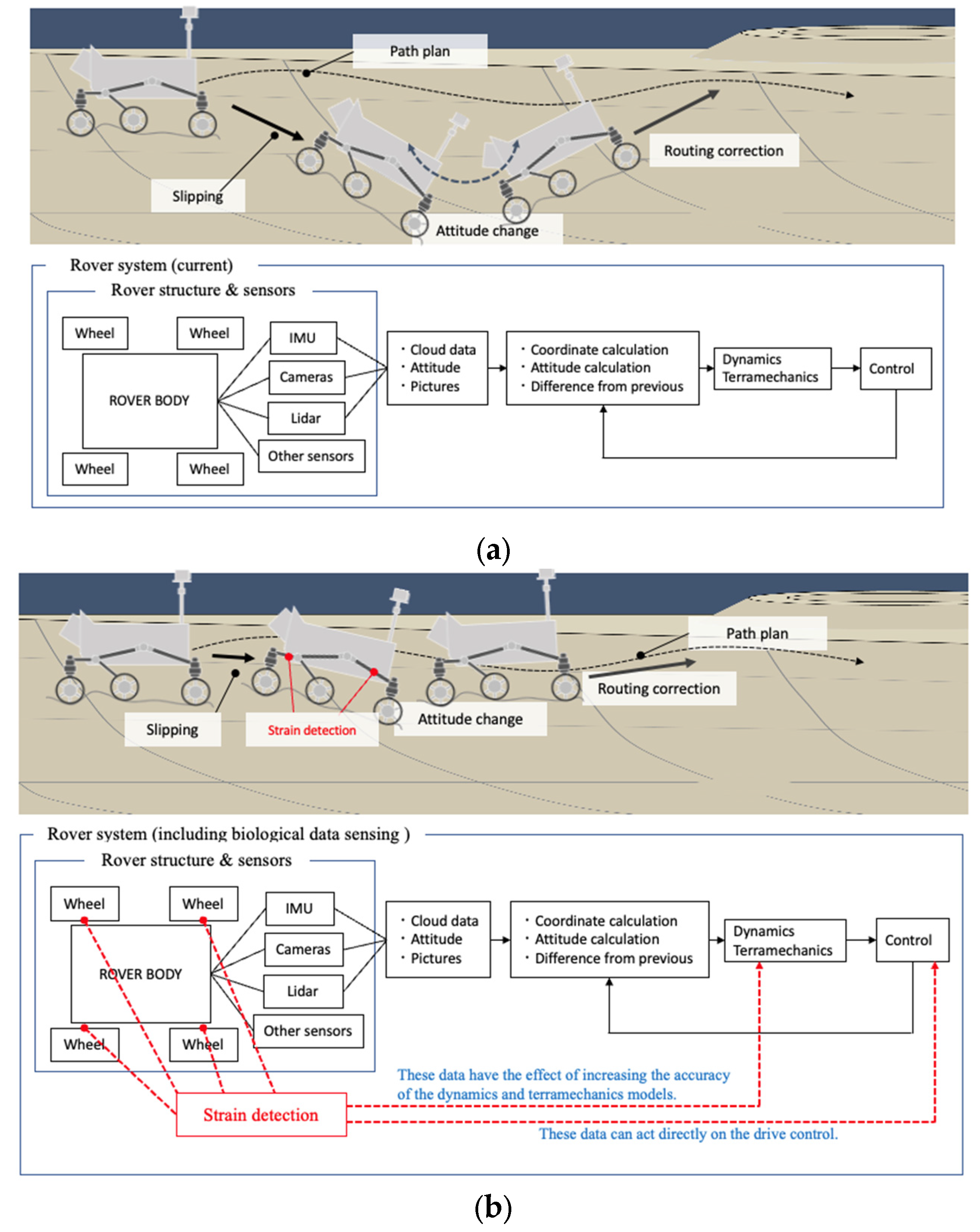
The current system would be greatly improved if important information related to driving, such as slip state and traction, could be obtained directly from the strain information for each wheel. When correcting a route based on sensing such as images, Lidar, and IMU, it is necessary to know the conditions of the wheels before and after the movement. Since the proposed system can obtain real-time information on the stimuli received by the body of the rover when the wheel rotates and contacts the ground, it is assumed that the path correction can be performed more quickly by incorporating them into the current system. Figure 5 indicates the current system (Figure 5a) and the advanced system with the strain detection processing unit (Figure 5b). In the present system, SLAM, which is based on the information from Lidar and cameras, is used to control the traveling of the rover, correct the route, and change the attitude. However, this is a calculation for the entire rover and cannot accurately identify the traction by each wheel. As Figure 5b shows, if the slip state and traction of each wheel are known, the accuracy of the dynamics and terramechanics models of the system can be improved. It would also be possible to control the rover directly in a reflexive manner (the strain data becomes large instantaneously, or the derivative value of the strain data is large, and so on). Thus, if the slip state and traction of each wheel can be estimated, it is expected that path correction can be performed with high accuracy for the rover. Even at present, a fast calculation may be performed, although it depends on the sampling period route and coordinates deviate from the planned ones. In such cases, the motion and drive to correct the path are calculated by using the terramechanics model.
3. Measurement
In this chapter, the strains acting on the chassis when the wheel travels are verified by experiments in which the wheel travels. Then, based on the experimental results, the method of analyzing the strain during traveling is discussed.
3.1. Experimental Environment and Conditions
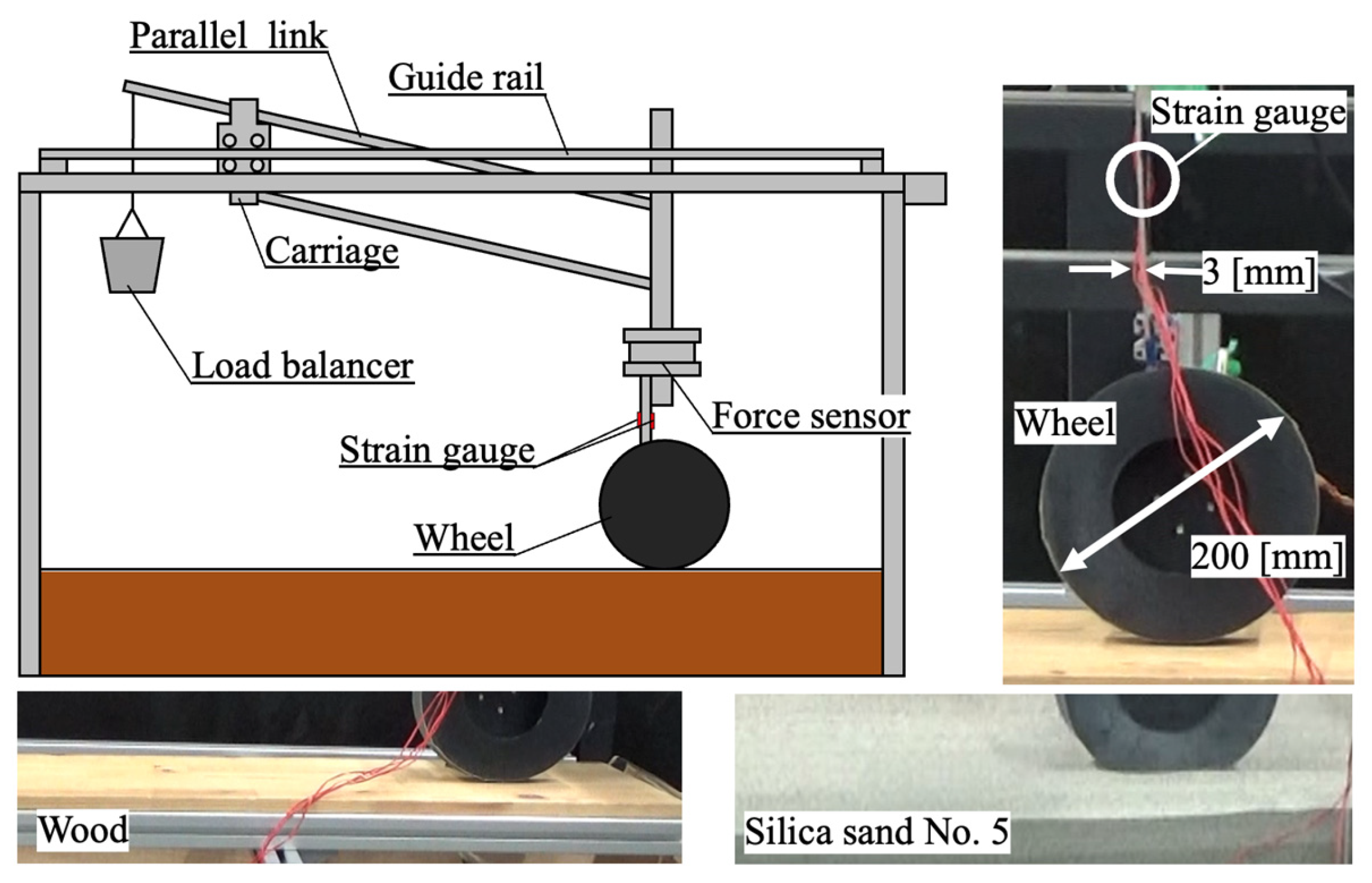
The strains on the chassis are measured by traveling the wheels on different ground surfaces, and the strains on the chassis during traveling are confirmed. Figure 6 shows the experimental environment and the single-wheel test bed. Two types of ground are used: loose soil and rigid ground. The loose soil is simulated by spreading silica sand No. 5 (Table 1), and the rigid ground is simulated by installing wood. In this study, we are focusing on the use of the movement of the ground, which is the breaking and shearing of the ground, in order to compare it with rigid ground. For this purpose, silica sand No. 5 is used. Moreover, the diameter of the wheel used in the experiment is 200 mm without a grouser (grousers are paddle-like objects attached to the surface of a wheel). This is in reference to a MER (Mar Exploration Rover (NASA/JPL) wheel (with grouser) with a wheel diameter of 250 mm. The strains are measured by strain gauges. The strain gauges are attached to the top of the chassis plate, where it is easiest to detect the strain, using a two-gauge method that is not really affected by external influences. The thickness of the chassis plate is 3 mm in order to have very low rigidity and to change the strain more easily. Figure 7 shows the strain measurement state and Table 2 shows the experimental conditions.
3.2. Results
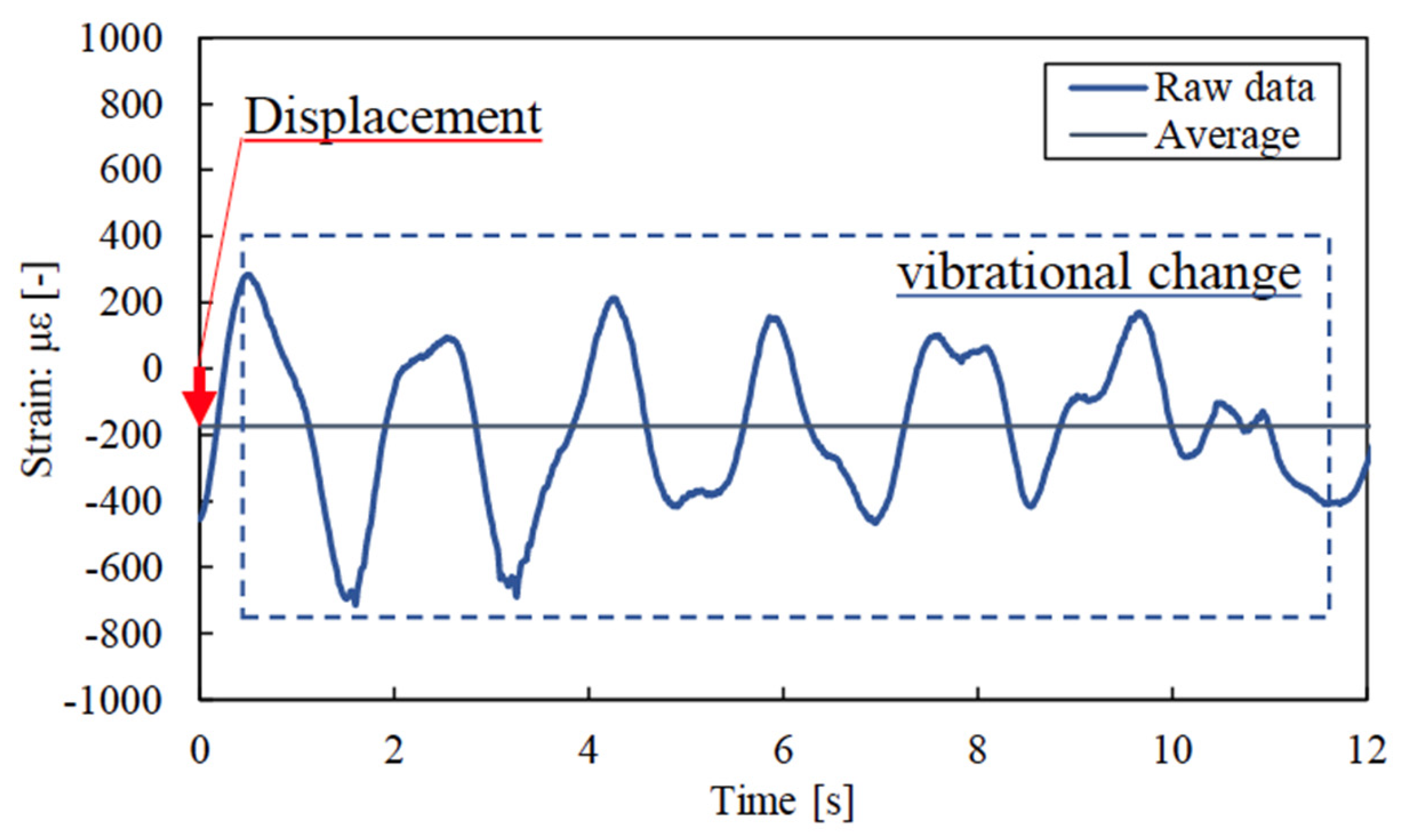
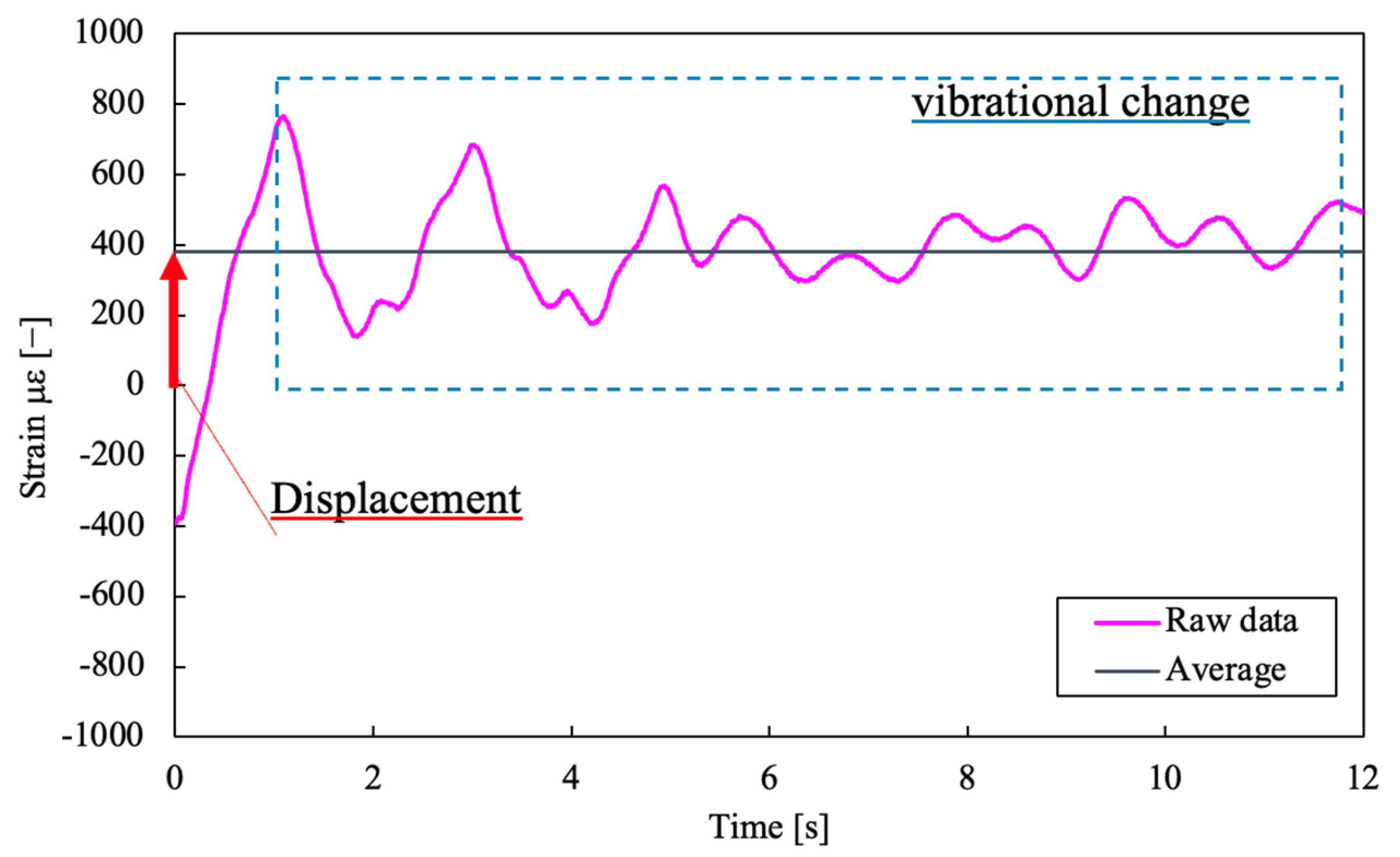
Figure 8 and Figure 9 show the change in strain when the wheel travels on each ground. The results of one trial are shown because the trend is similar for the five trials of each ground. When the strain is positive, the shape is changed by tilting the wheel forward, and when it is negative, the shape is changed by tilting the wheel backward. From the experimental results, different strain changes were confirmed for each ground. These strain changes are classified into two categories. The first is the displacement of the strain amount, and the second is the vibrational change in the strain. Based on these two categories, the analysis method of the strain during traveling is discussed in the next section.
3.3. Discussion
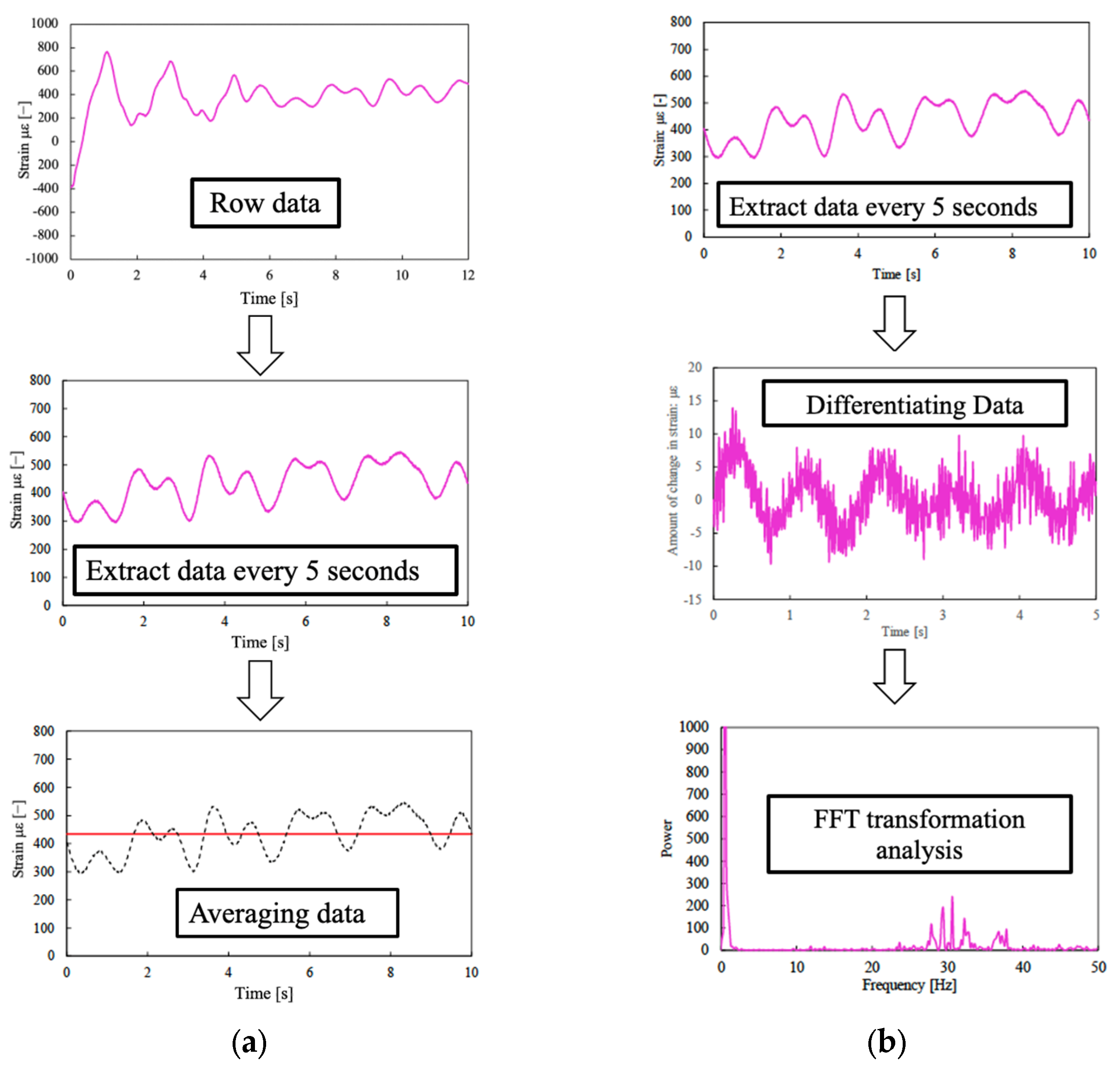
From the experimental results, the strains during traversing are classified into two major categories: the first is the displacement of the strain amount, and the second is the vibrational change in the strain. The analysis method is discussed from these results. We focus on muscle spindles, which are human receptors. There are intrinsic receptors called muscle spindles inside the human muscle to receive the stimulus of the chassis as shown in Figure 10 [38,39]. Muscle spindles are receptors in skeletal muscle. It is cylindrical in shape, thick in the middle, and gradually thinning at both ends (spindle shape). The muscle spindle has a role in sensing the rate of muscle fiber expansion and contraction. The capsule of the muscle spindle contains fibers called “nuclear chain fiber” and “nuclear bag fiber”. Nuclear bag fibers are bulging in the center, and nuclear chain fibers are rod-shaped. A single muscle spindle encapsulates two to three nuclear bag fibers and about five nuclear chain fibers. While muscle fibers are 20 to 100 μm in diameter and 2.5 to 30 cm in length, nuclear bag fibers are 12 to 25 μm in diameter and 7 to 10 mm in length, and nuclear chain fibers are 12 μm in diameter and 4 mm in length. Both ends of nuclear bag fibers exit the capsule and attach to the myointimal or tendon. “Group I afferent” mainly transmits information on the rate of change, while “Group II afferent” transmits information on length to the central nervous system. “γ motor” neurons contract the contractile tissue of intramuscular fibers and modulate their sensitivity to stretch. They are especially active when the muscle is shortened. The nuclear chain fiber can detect the displacement of absolute tension and is mainly used to recognize static phenomena such as postural states. The nuclear bag fibers can detect the speed of muscle fiber stretching and are mainly used to recognize dynamic phenomena. Thus, humans use intrinsic receptors “muscle spindles” to sense posture and walking state from the rate of displacement and stretch of muscle fibers. Therefore, the detection of displacement and velocity, which are the characteristics of muscle spindles, will be applied to a rover. This means that the resistance force and vibration transmitted from the ground when the wheels rotate are also transmitted to the chassis of the rover, and this mechanical information is used for detection like muscle spindles. Figure 11 shows the flow of our analysis. Raw data by time are indicated on top of Figure 11a. Then the data are extracted every 5 s. These data are then averaged. This flow is a “nuclear chain fiber”-like approach. Next, as shown in Figure 11b, a “Nuclear bag fiber”-like analysis approach is as follows. The raw data are extracted every 5 s (this is the first setup). Then, these data are differentiated. Finally, FFT analysis is performed on these data.
4. Verification
In this chapter, the strain on the chassis when the traveling state changes is verified by experiment. Then, the interrelationship between the traveling state and the strain is verified by two methods: the nuclear chain fiber method and the nuclear bag fiber method.
4.1. Experimental Environment and Conditions
The same test apparatus as in Section 2 is used for the experiments with wheels for the proposed analytical method. In addition, a traction load is applied to the wheels to reproduce slipping. The significance of applying a traction load is as follows. When a wheel slips, the sand under the wheel is scraped to the rear. At the same time, the wheel sinks into the sand while moving forward. As it sinks into the sand, the surface for traveling is angled. In other words, sinking could be considered to be equivalent to traversing on a slope. When traveling on a slope, the rover is subject to the effects of gravity. In other words, the rover is subjected to a traction load. Lunar and Mars rovers must travel and explore various slope-angle terrains, including inside and outside of craters, and the rover chassis is always subjected to traction loads. Therefore, it is very important to conduct traversing experiments that apply a traction load to the wheels. Moreover, in order to verify the interrelationship between the traveling condition and the strain on the chassis, the strain is measured when the traveling ground and the traveling state (forced slip condition by towing) are changed and verified by the nuclear chain fiber method and nuclear bag fiber method. In this experiment, the strains are measured by changing the vertical force: Fz for loose soil and rigid ground, and by changing the slip ratio: s for loose soil. The slipping ratio is the ratio calculated using the wheel’s actual translational velocity V and the peripheral velocity (ideal velocity of the wheel) of the wheel Vω as follows:
As the slip ratio is close to 1, it is difficult for the rover to move forward, and as it is close to 0, the wheel is moving forward.
Figure 12 shows the experimental environment. Figure 12 is a schematic diagram of a testing machine that travels a single wheel on the ground. The weight of the wheel can be actively adjusted by the parallel link and balancer. Vertical movement is also free by the parallel link. The single wheel is connected to a DC motor and its speed is controlled by PID control. During traveling, forward/backward and up/down movements are measured by motion capture. By towing the wheel from the rear, the wheel is made to slip actively, and the strain data are measured. The diameter of the wheel used in the experiment is 200 mm without grouser. This is in reference to a MER (Mars Exploration Rover (NASA/JPL)) wheel (with a grouser) with a wheel diameter of 250 mm. The vertical drag force is changed by changing the load of the load balancer to 18 N, 27 N, 36 N, and 54 N, and the slip ratio is changed by changing the load of the traction load to 0 g, 100 g, 200 g, and 300 g. The loose soil is simulated by spreading silica sand No. 5, and the rigid ground is simulated by installing wood. A motion capture system is used to measure the moving speed of the wheels. The test bed is the same as the one used in the experiment in Section 3. Table 3 shows the detailed experimental conditions.
4.2. Experimental Results: Nuclear Chain Fiber Method
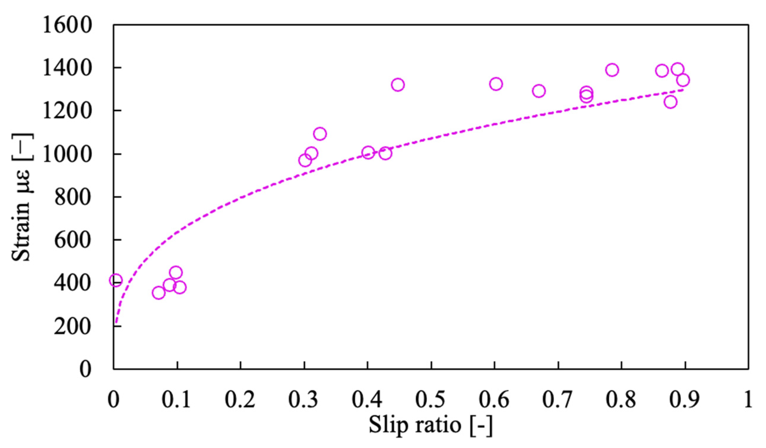
In order to verify, Figure 13 shows the results of the nuclear chain fiber analysis for each type of ground when the vertical force is changed. In both loose soil and rigid ground, the average value of the strain displacements changes linearly with the increase in vertical force. Figure 14 shows the results of the nuclear chain fiber analysis of loose soil when the slip rate is changed. The strain changes logarithmically with the increase in the slip rate. Figure 15 shows a graph of the driving force (drawbar pull) with the change in the slip rate and a graph of the strain with the change in the driving force (drawbar pull). The driving force (drawbar pull) is increasing logarithmically as well as the strain, thus the average value of the strain displacements changes linearly with the increase in driving force (drawbar pull). As a result, from the relationship that the strain increases linearly with the increase in the vertical force and the driving force (drawbar pull), it is possible to detect the change in the force applied to the wheel during traveling from the strain. Therefore, it is possible to recognize the traveling state by using the nuclear chain fiber analysis to detect the change in the force applied to the wheel during traveling.
4.3. Experimental Results: Nuclear Bag Fiber Method
Figure 16 and Figure 17 show the results (FFT analysis) of the nuclear bag fiber evaluation for each ground when the vertical force was changed. The results of one trial are shown because the trend is similar for the five trials of each ground. Even though the load changed, both loose ground and rigid ground responded strongly in the low-frequency range between 0–10 Hz. The loose soil also responded strongly in the higher frequency range between 20–50 Hz.
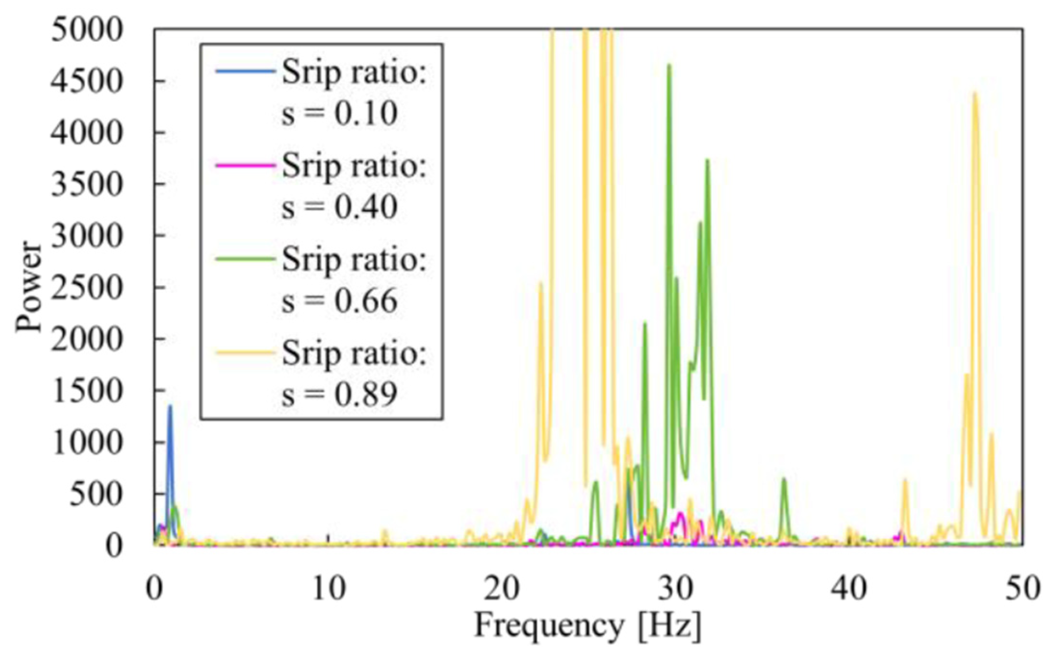
Figure 18 shows the results of the nuclear bag fiber analysis when the slip ratio was changed by changing the traction load in loose soil. As in the case of load change, a response was observed in the low-frequency range between 0 and 10 Hz, and this response decreased as the slip rate increased. As the slip rate increased, the response increased at a higher frequency between 20 and 50 Hz.
Therefore, different responses were measured in the low-frequency and high-frequency ranges by changing the traveling environment and conditions. This result is discussed.
The spectrum in the low-frequency range is discussed. The spectrum was larger for both rigid ground and loose soil, and the spectrum decreased with increasing slip ratio for loose soil. This phenomenon in the low-frequency range is caused by the vibration from the elastic deformation of the chassis during traveling. The displacement of the chassis increases with the speed because the traveling speed is kept in the state where the slip ratio is small. However, as the slip ratio increases, the traveling speed decreases, and the displacement of the chassis per time decreases. Therefore, as the slip ratio increased, the response decreased in the low-frequency range.
4.4. Slip Ratio Estimation Using Biological Processing (Nuclear Chain Fiber Method and Nuclear Bag Fiber Method)
The relationship between the strain data of the chassis and slip ratio, which was given arbitrarily, was derived experimentally. This means that there is no need to measure the displacement of the rover on the spot for the calculation of the slip ratio. If the information computed data of the strain is obtained on the spot, the slip state of the rover can be estimated for each wheel. From the analysis data given the nuclear chain fiber method and nuclear bag fiber method, we propose the slip ratio estimation. The estimation method is defined for each slip ratio level as follows. The slip ratio represents s.
(i) The estimation using the nuclear chain fiber method (use of average values of strain data).
0.0 < s < 0.4: The estimation with high accuracy is possible.
The slip ratio is obtained from the correlation as shown in Figure 14.
s > 0.4: The estimation with low accuracy is possible.
When the slip ratio becomes over 0.4, the strain data does not match the correlation.
(ii) The estimation using the nuclear bag fiber method (use of FFT analysis data of strain vibration).
Determining road condition while driving: The road condition (rigid surface or loose soil) can be judged by confirming the existence of a power spectrum (under 200 dB) extracted by FFT at the range 10–50 Hz of frequency as shown in Figure 17 and Figure 18.
s = 0.1: The slip ratio 0.1 can be judged by confirming the existence of a power spectrum (under 200 dB) extracted by FFT at the range 10–50 Hz of frequency as shown in Figure 18.
s = 0.4: The slip ratio 0.4 can be judged by confirming the existence of a power spectrum (under 500 dB over 200 dB) extracted by FFT at the range 10–50 Hz of frequency as shown in Figure 18.
s = 0.66: The slip ratio 0.66 can be judged by confirming the existence of a power spectrum (over 2000 dB) extracted by FFT at the range 20–40 Hz of frequency as shown in Figure 18.
s = 0.89: The slip ratio 0.89 can be judged by confirming the two existence of a power spectrum (over 2000 dB) extracted by FFT at the range 20–40 Hz and 40–50 Hz of frequency as shown in Figure 18.
Although this paper is treated with a 4-typed slip ratio, a lot of patterns of the slip ratio can be available by making the correlation between frequency and power spectrum with the slip ratios obtained using various towing masses.
Moreover, in general, it is necessary to calculate the slip ratio from the odometry data and locomotion data obtained from measurement systems like SLAM. However, the proposed method only measures the strain data on the spot. By the way, there are two waves in the range of 20–40 Hz and 40–50 Hz on a slip ratio of 0.89. In the next section, the particles of the soil flow in the low slip state and the high slip state are visualized to consider the difference between these two patterns of the slip ratio.
4.5. Visualization of Motion of Soil Grain in the Low Slip State and High Slip State
The spectrum in the high-frequency range is discussed. The spectrum is large on loose soil, and this spectrum increases with the increase in slip ratio. This phenomenon in the high-frequency range is caused by the movement of the particles in contact with the wheels during traveling.
In this visualization, a technique called PIV (particle image velocimetry) is used. As shown in Figure 19, the motion of particles is captured by PIV, and the direction and velocity of particle motion are measured by analyzing two consecutive images of particle groups [40]. In this experiment, visualization of soil grain moved by the rotation of a wheel is performed. In this visualization, a technique called PIV (particle image velocimetry) is used. The devices and software used for PIV are listed in Table 4.
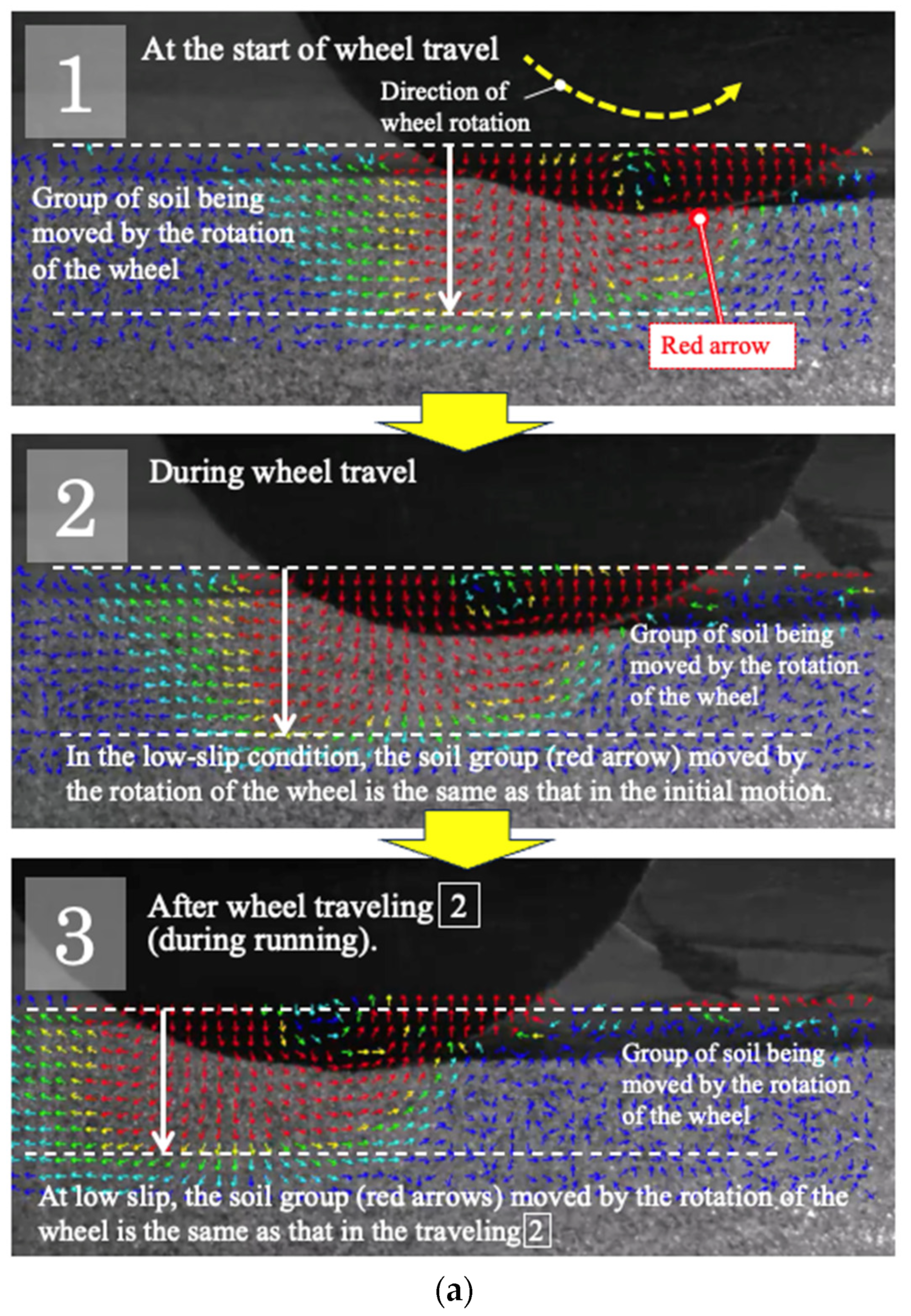
Figure 20 shows the motion of the particles when traveling on loose soil at two kinds of slip rates (low slip and high slip). The arrows display the direction of the soil grain and the magnitude of the soil flowing. The color of the arrow changes from blue to red as the flow magnitude increases. In the case of a low slip rate, the sand group being moved under the wheel (the area indicated by the red arrow) is always constant from the beginning of the rotation, as can be seen in Figure 20. This means that the shear stress acting on the contact condition between the wheel surface and the soil is easily stabilized. This is because, as shown in Figure 20a, soil grains moving on the wheel surface have the same velocity vector. This means that the wheel chassis vibration caused by the contact resistance is stable. As a result, the spectra that appear in the high-frequency region, such as the slip ratio of 0.4 shown in Figure 18, tend to gather in one place. However, in the case of high slip rates, the phenomenon changes. Wheels with high slip rates tend to be buried in the soil. This means that the area of soil in contact with the wheel surface increases. In these traveling experiments, the slip ratio is adjusted by traction, but when the wheels are buried in the soil, the resistance of the soil against the direction of travel increases. In other words, it becomes more and more difficult to move forward at the same time. Figure 20b shows that the soil group under the wheel (the area indicated by the red arrow) is decreasing as the wheel starts to travel. As the slip rate increases, the ground actively collapses by the wheels, and the fine vibrations caused by the ground collapse are transmitted to the vehicle body. In other words, in the high slip condition, there are complex groups of touching soil grain with various velocity vectors on the surface of the wheel. This means that the shear stress acting on the contact condition between the wheel surface and the soil is less stable than in the low slip condition. Furthermore, when the slip ratio is 0.89, we can see that the range is broken up.
5. Conclusions
In this paper, in order to develop a new system that focuses on human’s intrinsic senses to recognize the traveling state of rovers exploring the Moon and planets, we verified experimentally the interrelationship between the traveling state (slip condition) and the strain, which is the shape change in the chassis. The results of the verification are as follows.
- (1)
- The strains during traversing are classified into two major categories: the first is the displacement of the strain amount, and the second is the vibrational change in the strain. Based on the muscle spindle function, which is an intrinsic receptive sense, strain displacement was analyzed as a nuclear chain fiber analysis, and strain velocity was evaluated as a nuclear bag fiber analysis.
- (2)
- The results of nuclear chain fiber analysis are described. A linear relationship was found between the strain amount and the increase in the vertical and driving direction forces, and the increase or decrease in each force could be detected from the strain amount. Therefore, it is possible to recognize the traveling state (slip condition) by using the nuclear chain fiber analysis to detect the change in the force applied to the wheel during traveling.
- (3)
- The results of nuclear bag fiber analysis are described. The phenomenon that changes with the change in slip rate could be detected from the strain rate. Therefore, it is possible to recognize the traveling state (slip condition) by using the nuclear bag-fiber evaluation to detect the slip state. In this way, it was proved that the strain, which is a change in the shape of the chassis, can detect changes in the traveling state (slip condition).
In order to safely realize the travel control of an autonomous rover, it is necessary to take various environments into consideration in advance. For example, a crater has a central hill and a slope at its edge. In addition, there are many rocks and stones. In an environment with rocks and stones, the current sensor system is sufficient to detect them and to avoid or step over them. On the other hand, it is also possible that the relationships acquired on the ground may be different from those of actual regolith traveling. Since our proposal aims to derive the relationship between the driving conditions and changes in the rover chassis, it is an innovative idea that also assumes the possibility of updating this relationship in the field. During rover route planning [41] the experiences from the model used in this work should be also considered to make travel safe.
In the future, the relationship between traversing state and strain will be verified by traveling experiments using a four-wheel rover. In addition, a system that recognizes the traveling state (slip condition) from changes in chassis strain will be developed.
Author Contributions
K.I. (Kojiro Iizuka) and K.I. (Kohei Inaba) proposed the methodology. K.I. (Kohei Inaba) implemented it, did experiments and analysis, and wrote the original draft manuscript. K.I. (Kojiro Iizuka) supervised the study, directly contributed to the problem formulation, experimental design, and technical discussions, reviewed the writing, and gave insightful suggestions for the manuscript. All authors have read and agreed to the published version of the manuscript.
Funding
This work was supported by JSPS KAKENHI Grant Number JP21K03952.
Data Availability Statement
Not applicable.
Conflicts of Interest
The authors declare no conflict of interest.
References
- Otuki, M.; Wakabayashi, S.; Isigami, G.; Sutoh, M. Current status of, and challenges in relation to, the development of planetary exploration rovers at JAXA. J. Robot. Soc. Jpn. 2014, 32, 408–411. [Google Scholar] [CrossRef]
- Heinicke, C.; Adeli, S.; Baqué, M.; Correale, G.; Fateri, M.; Jaret, S.; Kopacz, N.; Ormö, J.; Poulet, L.; Verseux, C. Equipping an extraterrestrial laboratory: Overview of open research questions and recommended instrumentation for the Moon. Adv. Space Res. 2021, 68, 2565–2599. [Google Scholar] [CrossRef]
- Zuber, M.T.; Head, J.W.; Smith, D.E.; Neumann, G.A.; Mazarico, E.; Torrence, M.H.; Aharonson, O.; Tye, A.R.; Fassett, C.I.; Rosenburg, M.A.; et al. Constraints on the volatile distribution within Shackleton crater at the lunar south pole. Nature 2012, 486, 378–381. [Google Scholar] [CrossRef]
- Changela, H.G.; Chatzitheodoridis, E.; Antunes, A.; Beaty, D.; Bouw, K.; Bridges, J.C.; Capova, K.A.; Cockell, C.S.; Conley, C.A.; Dadachova, E.; et al. Mars: New insights and unresolved questions. Int. J. Astrobiol. 2021, 20, 394–426. [Google Scholar] [CrossRef]
- Kubota, T. Mobile Explorer Robot (Rover) for Lunar or Plenetary Exploration. J. Soc. Mech. Eng. 2001, 104, 71–74. [Google Scholar]
- Brusnikin, E.S.; Kreslavsky, M.A.; Zubarev, A.E.; Patratiy, V.D.; Krasilnikov, S.S.; Head, J.W.; Karachevtseva, I.P. Topographic measurements of slope streaks on Mars. Icarus 2016, 278, 52–61. [Google Scholar] [CrossRef]
- Kereszturi, A. Polar Ice on the Moon. In Encyclopedia of Lunar Science; Springer: Berlin/Heidelberg, Germany, 2023; pp. 971–980. [Google Scholar] [CrossRef]
- Morse, Z.R.; Osinski, G.R.; Tornabene, L.L.; Bourassa, M.; Zanetti, M.; Hill, P.J.; Pilles, E.; Cross, M.; King, D.; Tolometti, G. Detailed Morphologic Mapping and Traverse Planning for a Rover-based Lunar Sample Return Mission to Schrödinger Basin. Planet. Sci. J. 2021, 2, 167. [Google Scholar] [CrossRef]
- Hady, G.G.; Abigail, C.D.; Sebastian, H.; Andrea, A.; Damian, B. ALCIDES: A novel lunar mission concept study for the demonstration of enabling technologies in deep-space exploration and human-robots interaction. Acta Astronaut. 2018, 151, 270–283. [Google Scholar] [CrossRef]
- Marteau, E.; Wehage, K.; Higa, S.; Moreland, S.; Meirion-Griffith, G. Geotechnical assessment of terrain strength properties on Mars using the Perseverance rover’s abrading bit. J. Terramechanics 2023, 107, 13–22. [Google Scholar] [CrossRef]
- Da Poian, V.; Lyness, E.; Danell, R.; Li, X.; Theiling, B.; Trainer, M.; Kaplan, D.; Brinckerhoff, W. Science Autonomy and Space Science: Application to the ExoMars Mission. Front. Astron. Space Sci. 2022, 9, 848669. [Google Scholar] [CrossRef]
- Tang, Z.; Liu, J.; Wang, X.; Ren, X.; Chen, W.; Yan, W.; Zhang, X.; Tan, X.; Zeng, X.; Liu, D.; et al. Physical and mechanical characteristics of lunar soil at the Chang’E-4 landing site. Geophys. Res. Lett. 2020, 47, e2020GL089499. [Google Scholar] [CrossRef]
- Ding, L.; Zhou, R.; Yuan, Y.; Yang, H.; Li, J.; Yu, T.; Liu, C.; Wang, J.; Li, S.; Gao, H.; et al. A 2-year locomotive exploration and scientific investigation of the lunar farside by the Yutu-2 rover. Sci. Robot. 2022, 7, eabj6660. [Google Scholar] [CrossRef]
- Kubota, T. Rover Design for Lunar or Planetary Exploration. J. Robot. Soc. Jpn. 1999, 17, 609–614. [Google Scholar] [CrossRef]
- NASA/JPL. Spirit & Opportunity Highlights. 2004. Available online: http://mars.nasa.gov/mer/home/ (accessed on 20 August 2022).
- Helmick, D.M.; Cheng, Y.; Clouse, D.S.; Matthies, L.H.; Roumeliotis, S.I. Path following using visual odometry for a mars rover in high-slip Environments. IEEE Aerosp. Conf. Proc. 2004, 2, 772–789. [Google Scholar]
- Goldberg, S.B.; Maimone, M.W.; Matthies, L. Stereo vision and rover navigation software for planetary exploration. Proc. IEEE Aerosp. Conf. 2002, 5, 2025–2036. [Google Scholar]
- Xiong, Y.; Matthies, L. Error analysis of a real-time stereo system. In Proceedings of the IEEE Computer Society Conference on Computer Vision and Pattern Recognition, San Juan, PR, USA, 17–19 June 1997; pp. 1087–1093. [Google Scholar]
- Otsu, K.; Otsuki, M.; Isigami, G.; Kubota, T. Terrain adaptive detector selection for visual odometry in natural scenes. Adv. Robot. 2013, 27, 1465–1476. [Google Scholar] [CrossRef]
- Carvalho, H.; Vale, A.; Marques, R.; Ventura, R.; Brouwer, Y.; Gonçalves, B. Remote inspection with multi-copters, radiological sensors and SLAM techniques. In EPJ Web of Conferences; Uppsala University: Uppsala, Sweden, 2018; Volume 170, p. 07014. [Google Scholar] [CrossRef]
- Chen, M.; Yang, S.; Yi, X.; Wu, D. Real-time 3D mapping using a 2D laser scanner and IMU-aided visual SLAM. In Proceedings of the 2017 IEEE International Conference on Real-Time Computing and Robotics (RCAR), Okinawa, Japan, 14–18 July 2017; pp. 297–302. [Google Scholar] [CrossRef]
- Wen, W.; Hus, L.; Zhang, G. Performance Analysis of NDT-based Graph SLAM for Autonomous Vehicle in Diverse Typical Driving Scenarios of Hong Kong. Sensors 2018, 18, 3928. [Google Scholar] [CrossRef] [PubMed]
- Aldibaja, M.; Yanase, R.; Kim, T.H.; Kuramoto, A.; Yoneda, K.; Suganuma, N. Accurate Elevation Maps based Graph-Slam Framework for Autonomous Driving. In Proceedings of the 2019 IEEE Intelligent Vehicles Symposium (IV), Paris, France, 9–12 June 2019; pp. 1254–1261. [Google Scholar] [CrossRef]
- Wong, J.Y.; Reece, A.R. Prediction of rigid wheel performance based on the analysis of soil–wheel stresses, Part II. Performance of towed rigid wheels. J. Terramechanics 1967, 4, 7–25. [Google Scholar] [CrossRef]
- Bekker, M.G. Introduction to Terrain-Vehicle Systems; University of Michigan Press: Ann Arbor, MI, USA, 1969. [Google Scholar]
- Hayami, T.; Kaneko, F.; Kizuka, T. Differences in the Function of Somatosensory-Motor Integration depend on the Motor Experiences. Bio Mech. 2008, 19, 47–56. [Google Scholar]
- Proske, U.; Gandevia, A.C. The kinaesthetic senses. J. Physiol. 2009, 587, 4139–4146. [Google Scholar] [CrossRef]
- The National Aeronautics and Space Administration (NASA). NASA’s Artemis Rover to Land Near Nobile Region of Moon’s South Pole. Available online: https://www.nasa.gov/press-release/nasa-s-artemis-rover-to-land-near-nobile-region-of-moon-s-south-pole (accessed on 25 October 2022).
- The European Space Agency (ESA). Advanced-Concept Robots. Available online: https://www.esa.int/ESA_Multimedia/Keywords/Description/Moon_rover/(result_type)/videos (accessed on 28 October 2022).
- The Japan Aerospace Exploration Agency (JAXA). Data Acquisition on the Lunar Surface with a Transformable Lunar Robot, Assisting Development of the Crewed Pressurized Rover. Available online: https://global.jaxa.jp/press/2021/05/20210527-1_e.html (accessed on 27 October 2022).
- Mandt, K.; Deutsch, A.; Colaprete, A.; Cohen, B.A.; Heldmann, J. South Pole PSRs as Volatile Time Capsules for the Earth-Moon System: How Artemis Science Begins Building on LRO and LCROSS with the VIPER Mission. In Proceedings of the AGU Fall Meeting, Chicago, IL, USA, 12–16 December 2022. [Google Scholar]
- Ishigami, G.; Miwa, A.; Nagatani, K.; Yoshida, K. Terramechanics-based model for steering maneuver of planetary exploration rovers on loose soil. J. Field Robot. 2007, 24, 233–250. [Google Scholar] [CrossRef]
- Jia, Z.; Smith, W.; Peng, H. Terramechanics-based wheel–terrain interaction model and its applications to off-road wheeled mobile robots. Robotica 2012, 30, 491–503. [Google Scholar] [CrossRef]
- Yoshida, K.; Watanabe, T.; Mizuno, N.; Ishigami, G. Terramechanics-based analysis and traction control of a lunar/planetary rover. In Field and Service Robotics; Springer: Berlin/Heidelberg, Germany, 2003. [Google Scholar] [CrossRef]
- Wong, J.Y.; Reece, A.R. Prediction of rigid wheels performance based on analysis of soil-wheel stresses, Part I. performance of driven rigid wheels. J. Terramechanics 1967, 4, 81–98. [Google Scholar] [CrossRef]
- Wong, J.Y. Theory of Ground Vehicles, 4th ed.; John Wiley & Sons: Hoboken, NJ, USA, 2008. [Google Scholar]
- Shirai, T.; Ishigami, G. Accurate Estimation of Wheel Pressure-Sinkage Traits on Sandy Terrain using In-wheel Sensor System. In Proceedings of the 12th International Symposium on Artificial Intelligence, Robotics and Automation in Space (iSAIRAS 2014), Montreal, QC, Canada, 17–19 June 2014. [Google Scholar]
- Gotoh, A. Postural Change due to Sensory Input. J. Kansai Phys. Ther. 2010, 10, 5–14. (In Japanese) [Google Scholar]
- Cheung, M.; Schmuckle, A. Multisensory postural control in adults: Variation in visual, haptic, and proprioceptive inputs. Hum. Mov. Sci. 2021, 79, 102845. [Google Scholar] [CrossRef] [PubMed]
- Watanabe, T.; Iizuka, K. Observation of Movement of Ground Particles Given Vibration When Rod Is Dragged. Int. J. Eng. Technol. 2022, 14, 1–8. [Google Scholar] [CrossRef]
- Akos, K. Geologic field work on Mars: Distance and time issues during surface exploration. Acta Astronaut. 2011, 68, 1686–1701. [Google Scholar] [CrossRef]
Figure 1.
Outline of the traveling state (slip condition) detection system.

Figure 2.
Terramechanics model for a single wheel.

Figure 3.
Overview of traversing state. (a) Traversing state on rigid surface. (b) Traversing state on loose soil.
Figure 3.
Overview of traversing state. (a) Traversing state on rigid surface. (b) Traversing state on loose soil.

Figure 4.
Deformation of chassis and one traction working.

Figure 5.
Improvement of driving performance of the current system and the proposed system with strain detection sensing. (a) Current rover’s system. (b) Rover system including strain detection sensing (proposed sensing).
Figure 5.
Improvement of driving performance of the current system and the proposed system with strain detection sensing. (a) Current rover’s system. (b) Rover system including strain detection sensing (proposed sensing).

Figure 6.
Overview of experimental setting for measurement chassis experiment.

Figure 7.
Actual condition of the experiment.

Figure 8.
State of strain at traveling rigid surface.

Figure 9.
State of strain at traveling loose soil.

Figure 10.
Schematic diagram of a muscle spindle.

Figure 11.
Analysis method. (a) Analysis with “nuclear chain fibers”-like approach. (b) Analysis with “nuclear bag fibers”-like approach.
Figure 11.
Analysis method. (a) Analysis with “nuclear chain fibers”-like approach. (b) Analysis with “nuclear bag fibers”-like approach.

Figure 12.
Overview of experimental setting for interrelationship verification experiment.

Figure 13.
Vertical force vs. strain.

Figure 14.
Slip ratio vs. strain.

Figure 15.
Comparison with drawbar pull. (a) Slip ratio vs. drawbar pull. (b) Drawbar pull vs. strain.
Figure 15.
Comparison with drawbar pull. (a) Slip ratio vs. drawbar pull. (b) Drawbar pull vs. strain.

Figure 16.
Results of frequency analysis for strains (changing vertical force, rigid surface).

Figure 17.
Results of frequency analysis for strains (changing vertical force, loose soil).

Figure 18.
Results of frequency analysis for strains (changing slip ratio, rigid surface).

Figure 19.
System of particle image velocimetry [41].
Figure 19.
System of particle image velocimetry [41].

Figure 20.
Motion of the particles at different slip rates. (a) Visualization of groups of soil grain at low slip conditions. (b) Visualization of groups of soil grain at high slip conditions.
Figure 20.
Motion of the particles at different slip rates. (a) Visualization of groups of soil grain at low slip conditions. (b) Visualization of groups of soil grain at high slip conditions.


Table 1.
Soil parameters and values (silica No. 5).
| Modulus (Unit) | Value | Name of Parameters |
|---|---|---|
| g (m/s2) | 9.81 | Earth gravity |
| γ (kg/m3) | 1430 | Soil density |
| ϕ (°) | 22.3–32.5 | Internal friction angle |
Table 2.
Experimental conditions at using single wheel testbed.
| Description | Value |
|---|---|
| Slope angle (°) | 0 |
| Rotation speed (rpm) | 5.0 |
| Traveling distance (mm) | 500.0 |
| Number of trials (-) | 5 |
| Wheel diameter (mm) | 200 |
Table 3.
Condition of interrelationship verification experiment.
| Description | Value | |
|---|---|---|
| Ground condition | Silica sand No. 5, On Woods | Silica sand No. 5 (Table 1) |
| Weight (N) | 18, 27, 36, 54 | 27 |
| Drawbar mass (g) | 0 | 0, 100, 200, 300 |
| Slope angle (°) | 0 | |
| Rotation speed (rpm) | 5.0 | |
| Traveling distance (mm) | 500.0 | |
| Number of trials (-) | 5 | |
| Wheel diameter (mm) | 200 | |
Table 4.
Specification of the high-speed camera and software.
| Camera Type | A/D10bit Monochrome (HAS-U1M) |
|---|---|
| Sensor | 1/2-inch CMOS |
| Shutter speed | Maximum 10 [μs] |
| Valid pixels | 1280 × 1024 |
| FPS | 60–4000 |
| Image processing software | Flownizer2D Ver.1.2.14 (DITECT Corporation, Oldbury, UK) |
Disclaimer/Publisher’s Note: The statements, opinions and data contained in all publications are solely those of the individual author(s) and contributor(s) and not of MDPI and/or the editor(s). MDPI and/or the editor(s) disclaim responsibility for any injury to people or property resulting from any ideas, methods, instructions or products referred to in the content. |
© 2023 by the authors. Licensee MDPI, Basel, Switzerland. This article is an open access article distributed under the terms and conditions of the Creative Commons Attribution (CC BY) license (https://creativecommons.org/licenses/by/4.0/).
Share and Cite
MDPI and ACS Style
Iizuka, K.; Inaba, K. Slip Estimation Using Variation Data of Strain of the Chassis of Lunar Rovers Traveling on Loose Soil. Remote Sens. 2023, 15, 4270. https://doi.org/10.3390/rs15174270
AMA Style
Iizuka K, Inaba K. Slip Estimation Using Variation Data of Strain of the Chassis of Lunar Rovers Traveling on Loose Soil. Remote Sensing. 2023; 15(17):4270. https://doi.org/10.3390/rs15174270
Chicago/Turabian StyleIizuka, Kojiro, and Kohei Inaba. 2023. "Slip Estimation Using Variation Data of Strain of the Chassis of Lunar Rovers Traveling on Loose Soil" Remote Sensing 15, no. 17: 4270. https://doi.org/10.3390/rs15174270
Note that from the first issue of 2016, this journal uses article numbers instead of page numbers. See further details here.