Deep Learning-Based Detection of Urban Forest Cover Change along with Overall Urban Changes Using Very-High-Resolution Satellite Images

Abstract

Urban forests globally face severe degradation due to human activities and natural disasters, making deforestation an urgent environmental challenge. Remote sensing technology and very-high-resolution (VHR) bitemporal satellite imagery enable change detection (CD) for monitoring forest changes. However, deep learning techniques for forest CD concatenate bitemporal images into a single input, limiting the extraction of informative deep features from individual raw images. Furthermore, they are developed for middle to low-resolution images focused on specific forests such as the Amazon or a single element in the urban environment. Therefore, in this study, we propose deep learning-based urban forest CD along with overall changes in the urban environment by using VHR bitemporal images. Two networks are used independently: DeepLabv3+ for generating binary forest cover masks, and a deeply supervised image fusion network (DSIFN) for the generation of a binary change mask. The results are concatenated for semantic CD focusing on forest cover changes. To carry out the experiments, full scene tests were performed using the VHR bitemporal imagery of three urban cities acquired via three different satellites. The findings reveal significant changes in forest covers alongside urban environmental changes. Based on the accuracy assessment, the networks used in the proposed study achieved the highest F1-score, kappa, IoU, and accuracy values compared with those using other techniques. This study contributes to monitoring the impacts of climate change, rapid urbanization, and natural disasters on urban environments especially urban forests, as well as relations between changes in urban environment and urban forests.

1. Introduction

Urban forests, consisting of urban trees, grass, and forests, are components of urban ecosystems providing a full spectrum of services such as alleviating urban heat, enhancing air quality, reducing stormwater runoff, and reducing greenhouse gas emissions, benefiting humans directly or indirectly [1,2,3,4]. However, urban forests around the world are under the significant pressure of degradation due to various reasons, including natural disasters and human activities such as wildfires, floods, new constructions, or illegal logging [5]. As a result, these days deforestation has become one of the most intractable environmental problems [6]. Generally, deforestation monitoring is usually conducted through tedious manual procedures including visual inspections, which require frequent visits to forest regions and can be costly and dangerous [7].

In the last few decades, with the advancements in remote sensing technology and the availability of bitemporal satellite imagery, change detection (CD) is being used for forest change monitoring [8]. In traditional methods, either vegetation masks for bitemporal images are generated by using a conventional vegetation detection technique such as the normalized difference vegetation index (NDVI) [9], or CD is carried out by using traditional approaches such as pixel-based CD or object-based CD [10]. The NDVI takes advantage of different solar radiation absorption phenomena of green plants in the red and near-infrared spectral bands [11]. However, vegetation masks generated by NDVI from very-high-resolution (VHR) satellite images of urban environments can suffer from noise because of the abundance of detailed information in VHR imagery [12,13]. Furthermore, researchers have shown that pixel-based CD techniques are sensitive to noise because they do not fully consider the spatial context [14,15]. On the other hand, object-based CD approaches showed better accuracies [16]. However, the effectiveness of these approaches depends on image segmentation quality [17]. Because of the complex land cover types such as large urban areas in VHR satellite imagery, the over- and under-segmentation of objects occur, reducing the efficiency and accuracy of object-based CD techniques [17]. Moreover, these techniques are usually developed for a specific dataset or site, meaning that similar results cannot be achieved when applied to a new dataset or site [18].

The use of deep learning networks reduces the number of manual steps in monitoring changes via automating feature extraction, avoiding feature selection, and reducing manual steps during CD [19]. Recently, deep learning-based techniques have demonstrated considerable success in a range of applications, including segmentation and CD, particularly in the context of forest detection and forest change monitoring [20,21,22,23,24]. For example, researchers in [25] have performed forest cover CD in incomplete satellite images by using a deep neural network in a data-driven format for automatic feature learning. In another study, land cover classification and CD using Sentinel-2 satellite data were carried out in which a fully convolutional network was combined with a long short-term memory network [26]. A baseline Unet model and Sentinel-2 data for regular CD in a Ukrainian forest were used [27]. Furthermore, analysts introduced a semantic segmentation-based framework for forest estimation and the CD technique, in which multitemporal Landsat-8 images were employed into a trained U-net model, and binary forest cover maps were generated. Afterward, the pixel-wise difference between two binary maps (i.e., pre-change and post-change binary maps) was calculated for generating a change map [28]. In another study, forest CD in bi-temporal satellite images is performed by generating anenhanced forest fused difference image, extracting changed and unchanged regions of forest with a recurrent residual-based Unet network [29]. Moreover, coastal forest CD was carried out by using convolutional neural networks (CNNs) [30].

However, most of the CD networks are modified from networks that are proposed for single-image semantic segmentation tasks. In these networks, bitemporal images are concatenated in order to meet the requirement of a single image input because of which early fusion networks fail to provide the informative deep features of individual raw images for image reconstruction [31]. In [31], Zhang et al. addressed this problem by introducing a deeply supervised image fusion network (DSIFN) for CD in VHR imagery. In order to generate highly representative deep bitemporal features, feature extraction is conducted via an independently trained fully convolutional two-stream architecture [31]. Furthermore, among different semantic segmentation networks, analysts have demonstrated the effectiveness of Deeplabv3+ [32] for various types of vegetation extraction and detection [33,34,35,36,37,38]. With Deeplabv3+, high-level features of different scales can be extracted using atrous spatial pyramid pooling (ASPP). Additionally, Deeplabv3+ combines multiple features with the encoder–decoder approach, making it a highly efficient and accurate semantic segmentation method [39].

Earlier mentioned techniques either used low-resolution or middle-resolution satellite images in which small changes related to vegetation could be easily ignored or remain undetected. The final forest CD result may suffer from a large amount of false detections or miss detections when tested on VHR bitemporal imagery. Also, these studies focused on huge regions such as Amazon forests and did not consider forests around urban areas where changes in forest and other urban elements occur simultaneously due to rapid urban expansions. Additionally, forest changes in these regions are small compared to other change in an urban environment, and a deep learning technique used to directly detect changes in forest cover may suffer from the class imbalance problem because non-change regions in the scene will be huge compared to the changes in the forest region only. By utilizing pre- and post-change binary forest covers with a binary change mask, forest change can be monitored together with overall changes in an urban environment. Therefore, in this study, we addressed the priorly mentioned problems by benefiting from Deeplabv3+ and DSIFN. We introduced transfer learning-based forest change (i.e., increase or decrease) detection together with the detection of overall urban changes in VHR bitemporal satellite imagery in a semantic CD manner [40]. We trained the two networks independently on open-source datasets and then performed transfer learning using our own datasets. Trained Deeplabv3+ was used for the generation of binary forest masks from both pre- and post-change VHR images, while DSIFN was used for binary change mask generation.

The contributions of the proposed study are as follows: (1) the utilization of two networks for CD, in a semantic CD manner, in an urban environment while focusing on forest cover decrease as well as increase concerning overall changes in the scene, (2) the usage of VHR bitemporal imagery for deforestation detection, (3) the utilization of the detected binary forest mask of pre- and post-change imagery for reducing false detections, missed detections, and salt-and-pepper noise in the final result, and (4) the transfer learning of both networks trained on open-source datasets to our own VHR imagery dataset.

2. Datasets

For forest detection, a remote sensing land cover dataset for domain-adaptive semantic segmentation known as LoveDA [41] was used. The dataset consists of 2522 training images and 1669 validation images composed of 1024 × 1024 pixels with red, green, and blue bands. Labels have seven classes such as buildings, roads, water, barren, forest, agriculture, and background. However, as our task is related to urban forest detection, we extracted only the forest class from the labels and combined other classes with a background class. Moreover, due to memory issues, we cropped each image into four image patches of 512 × 512 pixels; the final dataset became 10,088 images for training and 6676 for validation with two classes (i.e., forest and background). For performing change detection, we used the dataset provided by the authors of DSIFN. Initially, the dataset consisted of 3600 images composed of 512 × 512 pixels with red, green, and blue spectral bands for training and 340 for validation. However, we reduced the image size to 128 × 128 pixels.

For the transfer learning of both networks and the evaluation of the proposed methodology, we generated datasets for each network from VHR bitemporal images of three sites acquired via three different satellites. The images were acquired over cities in South Korea such as Sejong, Daejeon, and Gwangju via Kompsat-3, QuickBird-2, and WorldView-3, respectively. The overall description of bitemporal images is provided in

Table 1. Specifications of VHR bitemporal satellite images.

Sites	Site 1 (Sejong)	Site 2 (Daejeon)	Site 3 (Gwangju)
Sensor	Kompsat-3	QuickBird-2	WorldView-3
Acquisition Date	Pre-change (16/11/2013) Post-change (26/02/2019)	pre-change (12/2002) Post-change (10/2006)	Pre-change (05/2017) Post-change (05/2018)
Spatial Resolution	2.8 m	2.44 m	1.24 m
Bands	Blue, green, red, NIR	Blue, green, red, NIR	Blue, green, red, NIR
Size	3879 × 3344 pixels	2622 × 2938 pixels	5030 × 4643 pixels

. Binary forest labels for each bitemporal image and binary CD labels were generated through the visual inspection and manual digitization of images. Bitemporal images together with binary forest labels are given in Figure 1, and their CD labels are shown in Figure 2. Briefly, 2800 image patches and corresponding label patches composed of 512 × 512 pixels for transfer learning for a forest detection network were generated from the bitemporal images of Sites 1 and 3. We extracted the patches with NIR, red, and green spectral bands because red and NIR bands give useful information regarding the vegetation in satellite images. Similarly, for the change detection network, 2800 image patches at a size of 128 × 128 pixels were generated with red, green, and blue spectral bands. The patches consisted of pre-change, post-change, and CD label images. Site 2 was utilized as the test dataset to evaluate the performance of transfer learning.

3. Methodology

The proposed method is mainly divided into three steps: (1) binary forest mask generation by using a well-known semantic segmentation technique, Deeplabv3+, (2) binary change mask generation through DSIFN, and (3) forest change monitoring with respect to overall changes in the scene. The flowchart of the proposed method is provided in Figure 3. VHR bitemporal images are independently employed in DeepLabv3+ for urban forest mask generation. At the same time, these images are given as inputs to DSIFN for binary change mask generation. Then, the three binary masks are combined to generate a semantic CD result and forest change is monitored with overall changes.

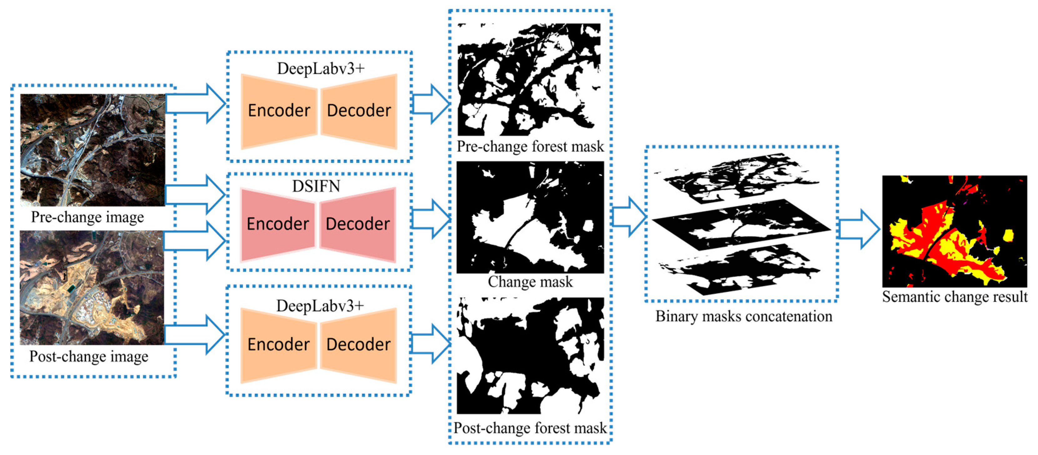
3.1. Binary Forest Mask Generation

In this study, to generate binary forest masks for VHR bitemporal satellite images, Deeplabv3+ was used. Deeplabv3+ is a semantic segmentation network designed for image classification at the pixel level and is developed for improving the segmentation results. It extends by adopting an encoder–decoder architecture and improving the decoder via the use of ASPP. The encoder uses a pre-trained CNN for generating high-level features from the input image. The input image passes through multiple convolutional layers for decreasing the spatial dimensions and enhancing the feature channels. Multi-scale contextual information is generated at the end of the encoder module by the ASPP. The decoder module is responsible for restoring the spatial resolution of a segmented image. This is achieved by upsampling the feature maps and incorporating fine-grained features between the encoder and decoder stages. Detailed information regarding the architecture of DeepLabv3+ can be found in [32].

In this study, ResNet-50 trained on ImageNet was used for extracting high-level features. Through a series of convolutional layers, the spatial dimensions of the images were reduced while enhancing the feature channels. ASPP generated feature maps that contained contextual information at different scales, and enhanced the model’s ability to understand and segment forest regions accurately. In the decoder module, the spatial resolution of the forest segmentation map was retrieved. This process ensured that detailed information was maintained during the upsampling process, resulting in a higher-resolution forest mask. Finally, pixel-level classification was performed using a sigmoid activation function. The sigmoid function transformed the pixel values to a range between 0 and 1, representing the probability of each pixel belonging to the forest class. To obtain a binary mask, a manual thresholding approach was employed in this study. Furthermore, both pre-change and post-change images were independently inputted into DeepLabv3+, and binary forest masks were then generated for each image. The overall architecture of binary forest mask generation is illustrated in Figure 4.

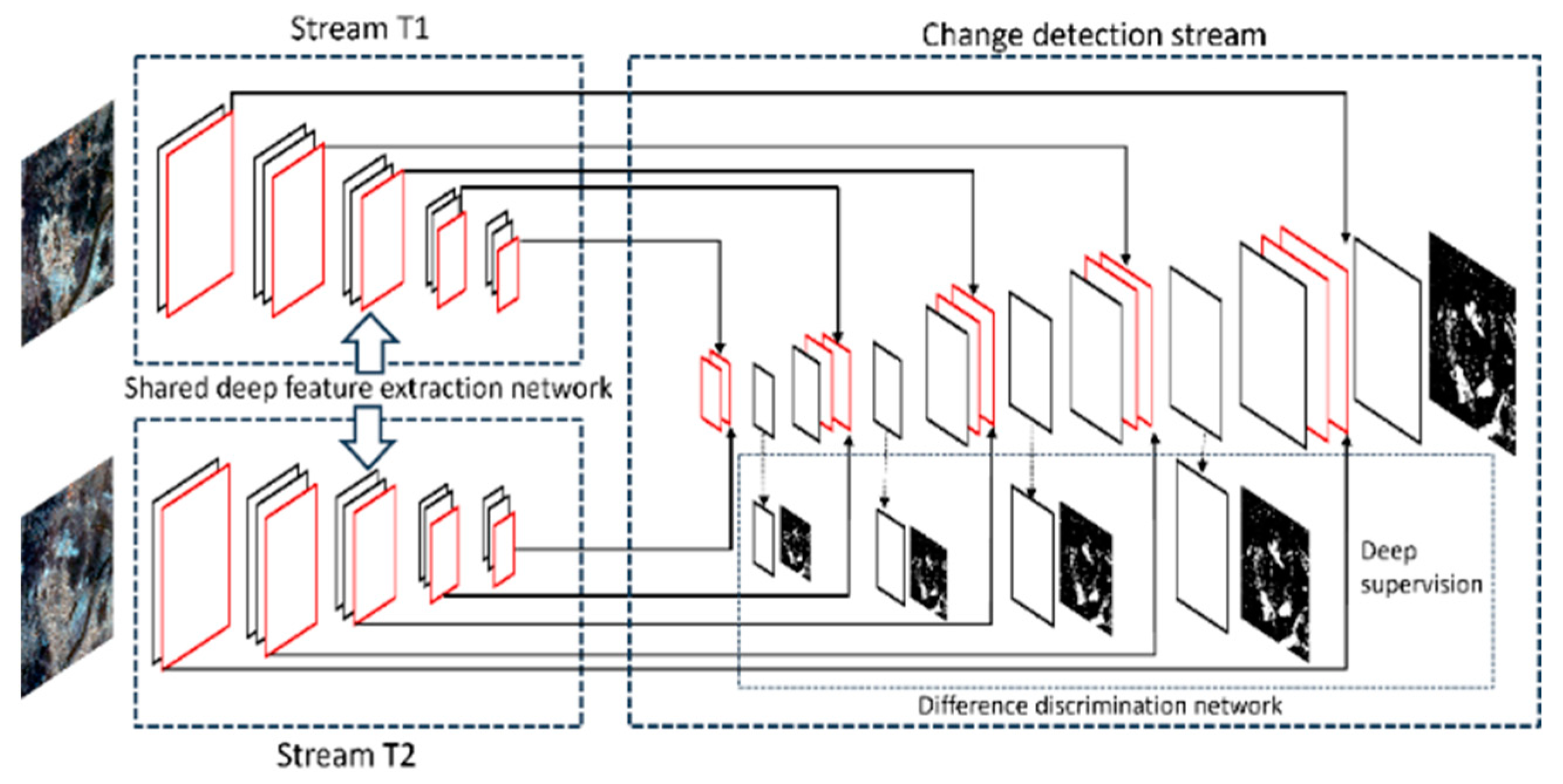
3.2. Binary Change Mask Generation

To generate a binary change mask, we used DSIFN introduced in [31]. The main idea behind the DSIFN is to develop a deep learning-based network that can effectively fuse information from two bi-temporal remote sensing images and perform CD. DSIFN preserves the change region boundaries and reconstructs high-quality maps by extracting deep bitemporal features independently and via the layer-wise concatenation of deep features and image difference features. DSIFN is divided into three streams. The first stream extracts deep features from the pre-change image using layers of a pre-trained VGG16 network. The second stream extracts deep features from the post-change image by sharing the structure and parameters of the first stream. The extracted features from pre- and post-change images are stacked at the same scales in order to supply both low-level and high-level raw image features to the third stream (i.e., CD stream). Overall, the first two streams consist of several convolutional layers each followed by a non-linear activation function such as the rectified linear unit (ReLU).

CD stream uses a difference discrimination network responsible for upsampling the features back to the original resolution and generating the fused CD map. The lowest layers of the first two streams acquire broad receptive fields and condense global information after progressive abstraction using layered convolutional and pooling layers. Therefore, the last layers of these streams serve as an initial input to the difference discrimination network to generate a preliminary global change map of a small size. Earlier layers that include the low-level information of input images are skip-connected to a difference discrimination network with the same scales. Three convolutional layers are applied to generate compact-sized difference image features. For features map refinement across the spatial dimensions, a spatial attention module is used. Then, the image difference feature maps are upsampled for enlarging feature maps. For fusing raw deep features with image difference features, a channel attention module is used. A detailed explanation regarding DSIFN can be found in [31]. The overall network architecture of DSIFN is provided in Figure 5.

3.3. Forest Change Monitoring

For generating the final semantic change result, firstly, pre- and post-change forest masks obtained through the proposed forest detection technique were separately utilized with a change mask generated via a change detection network (expressed in Equation (1)) for extracting the forest change pixels from the two forest masks. The pre- and post-change binary forest maps were used for identifying forest cover decrease (${\mathrm{F}\mathrm{o}\mathrm{r}\mathrm{e}\mathrm{s}\mathrm{t}}_{\mathrm{d}}$) and increase (${\mathrm{F}\mathrm{o}\mathrm{r}\mathrm{e}\mathrm{s}\mathrm{t}}_{\mathrm{i}}$).

$$\begin{gathered} {\mathrm{F}\mathrm{o}\mathrm{r}\mathrm{e}\mathrm{s}\mathrm{t}}_{\mathrm{d}}=\left\{\begin{array}{ll}1,& \hspace{1em}if {\mathrm{M}\mathrm{a}\mathrm{s}\mathrm{k}}_{\mathrm{T}1}\cap {\mathrm{M}\mathrm{a}\mathrm{s}\mathrm{k}}_{\mathrm{C}}=1\\ 0,& \hspace{1em}else\end{array}\right. \\ {\mathrm{F}\mathrm{o}\mathrm{r}\mathrm{e}\mathrm{s}\mathrm{t}}_{\mathrm{i}}=\left\{\begin{array}{ll}1,& \hspace{1em}if {\mathrm{M}\mathrm{a}\mathrm{s}\mathrm{k}}_{\mathrm{T}2}\cap {\mathrm{M}\mathrm{a}\mathrm{s}\mathrm{k}}_{\mathrm{C}}=1\\ 0,& \hspace{1em}else\end{array}\right. \end{gathered}$$

(1)

where ${\mathrm{M}\mathrm{a}\mathrm{s}\mathrm{k}}_{\mathrm{T}1}$ and ${\mathrm{M}\mathrm{a}\mathrm{s}\mathrm{k}}_{\mathrm{T}2}$ are the pre- and post-change binary forest masks, and ${\mathrm{M}\mathrm{a}\mathrm{s}\mathrm{k}}_{\mathrm{C}}$ denotes the change mask.

From Equation (1), after the integration of the two masks, a binary forest change map was generated (e.g., ${\mathrm{M}\mathrm{a}\mathrm{s}\mathrm{k}}_{\mathrm{T}1} {\mathrm{a}\mathrm{n}\mathrm{d} \mathrm{M}\mathrm{a}\mathrm{s}\mathrm{k}}_{\mathrm{C}}$ for the forest decrease map, and vice versa) by assigning 0 to the unchanged forest pixels and changed non-forest pixels, and 1 to the changed forest pixels. Via the aforementioned process, the forest maps’ pixels belonging to the change in the two masks could be preserved and the pixels related to non-change forest regions could be eliminated.

After concatenating the bitemporal binary forest increase and decrease masks and the binary CD mask, we created a comprehensive semantic change map as shown in Figure 6. The semantic change map provides a detailed representation of the forest cover changes during the specific period under consideration. The semantic change map includes four classes: forest cover increase, forest cover decrease, non-forest change regions, and falsely change regions.

3.4. Validation

To assess the overall extent of changes in the scene, we calculated the percentage of overall changed regions by dividing the total number of changed pixels in the semantic change map by the total number of pixels in the scene. To gain further insights into the forest cover changes, we analyzed the forest cover decrease and increase individually. The percentage of forest cover decrease is determined by dividing the total number of pixels indicating a decrease in forest cover by the total number of changed pixels in the semantic change map. Similarly, the percentage of forest cover increase is calculated by dividing the total number of pixels indicating an increase in forest cover by the total number of changed pixels. These metrics show the trend of forest cover change with respect to other urban changes.

Firstly, the two networks were trained independently on open-source datasets for each task. Then, transfer learning was performed using our dataset. Tests were carried out by using the full-scene bitemporal images of Site 2 as well as Sites 1 and 3. For the quantitative evaluation of networks used in this study, the F1-score, kappa, accuracy, intersection over union (IoU), false alarm rate (FAR), and miss rate (MR) were calculated using each predicted result and the manually digitized labels. The binary forest masks generated via DeepLabv3+ in this study were compared with the binary forest masks generated via Unet [42], SegNet [43], and the NDVI. Moreover, we compared the final semantic change detection result using the proposed method with the results generated by combining the change detection map in this study with the deforestation detection result generated by using unsupervised deforestation detection, which was introduced in [13].

4. Experimental Results

The networks were trained using Tensorflow, AMD Ryzen 7 5800X 8-Core Processor CPU with 64.0 GB RAM, and NVIDIA GeForce RTX 3060 GPU. Networks were trained via the open-source datasets on several epochs, and the ones with the best accuracies were chosen (i.e., 25 for DeepLabv3+, and 60 for DSIFN). A binary cross-entropy loss and an Adam optimizer were used for both networks. The minimum and maximum learning rates during training with a learning rate reduction for DeepLabv3+ were set to 0.000001 and 0.0001, and those for DSIFN were set to 0.000001 and 0.0001, respectively. The maximum learning rate was set differently for both networks according to the variations in the training and validation accuracies and losses. The batch size was set to 8 and 32 for DeepLabv3+ and DSIFN, respectively.

After training networks on open-source datasets, the final training and validation accuracies, and losses for DeepLabv3+ were 0.954 and 0.937, and 0.115 and 0.175, while those for DSIFN were 0.958 and 0.926, and 0.095 and 0.185, respectively.

Then, the transfer learning of both networks was performed using our own dataset. During transfer learning, the epochs with better accuracies achieved via DeepLabv3+, and DSIFN were 100, and 40, respectively. The training and validation accuracies of DeepLabv3+, and DSIFN were 0.942 and 0.903, and 0.991 and 0.972, respectively. Similarly, the losses were 0.148 and 0.267, and 0.022 and 0.087. The training and validation performance of the two neural networks are visually represented in Figure 7 and Figure 8, where accuracy and loss metrics are depicted.

4.1. Binary Forest Masks

Firstly, full scene binary forest masks were generated using the bitemporal images of the three sites. Patches were generated from the pre-change VHR image of each site. Then, a trained Deeplabv3+ network was used to predict and thus generate a forest cover mask from the patches. The resulting patches after prediction were combined to generate the same size result as that of the original image for each site. Afterward, multiple thresholds were tested and the one with the best results such as 0.4 was selected for binary forest mask generation. A similar process was repeated using a post-change VHR image. After binary forest mask generation for both (i.e., pre-change and post-change) images, we visually compared the results with the binary forest masks generated by using the NDVI. For generating the masks using the NDVI, a threshold with the best accuracy was selected. The binary forest masks generated via DeepLabv3+ in this study, and the NDVI from the pre-change image of each site are shown in Figure 9 along with label images.

Compared to the label images (i.e., Figure 9c,f,i) and the results generated via the NDVI (Figure 9a,d,g), the proposed method effectively detected forest covers shown in Figure 9b,e,h. Through a visual inspection, binary forest covers generated via the NDVI for all three sites have missed as well as falsely detected regions, which makes them seem like salt-and-pepper noise. Furthermore, in the binary results generated via the NDVI, trees or grass beside roads and streams are detected as forest covers, while the proposed method effectively differentiated between grass and forest. The quantitative assessment of predicted results using the proposed technique, Unet, SegNet, and the NDVI for bitemporal images at each site is presented in

Table 2. Quantitative assessment of predicted forest cover masks.

Site	Technique	Images	F1-Score	Kappa	IoU	Accuracy	FAR	MR
1	Proposed method	Pre-change	0.908	0.855	0.831	0.933	0.0679	0.0967
		Post-change	0.874	0.813	0.777	0.917	0.062	0.147
	Unet	Pre-change	0.887	0.831	0.797	0.924	0.089	0.099
		Post-change	0.849	0.778	0.738	0.903	0.082	0.123
	SegNet	Pre-change	0.902	0.843	0.822	0.925	0.120	0.098
		Post-change	0.774	0.686	0.631	0.871	0.092	0.186
	NDVI	Pre-change	0.789	0.665	0.753	0.840	0.198	0.079
		Post-change	0.825	0.724	0.694	0.870	0.160	0.064
2	Proposed method	Pre-change	0.915	0.887	0.844	0.958	0.032	0.68
		Post-change	0.902	0.872	0.821	0.952	0.037	0.080
	Unet	Pre-change	0.903	0.870	0.823	0.950	0.012	0.398
		Post-change	0.894	0.857	0.809	0.944	0.032	0.203
	SegNet	Pre-change	0.889	0.846	0.801	0.937	0.102	0.063
		Post-change	0.868	0.814	0.767	0.922	0.145	0.035
	NDVI	Pre-change	0.733	0.669	0.617	0.892	0.012	0.398
		Post-change	0.841	0.792	0.620	0.925	0.032	0.203
3	Proposed method	Pre-change	0.853	0.834	0.744	0.965	0.035	0.093
		Post-change	0.836	0.816	0.719	0.963	0.026	0.102
	Unet	Pre-change	0.827	0.801	0.705	0.954	0.047	0.099
		Post-change	0.820	0.792	0.695	0.950	0.059	0.102
	SegNet	Pre-change	0.823	0.799	0.699	0.958	0.124	0.098
		Post-change	0.774	0.746	0.618	0.951	0.102	0.120
	NDVI	Pre-change	0.643	0.601	0.551	0.924	0.037	0.429
		Post-change	0.525	0.475	0.473	0.905	0.039	0.546

. When comparing the forest masks extracted via Unet, SegNet, and the NDVI, the proposed method consistently demonstrated superior performance, as indicated by the higher F1-scores, kappa, IoU, and accuracy values across all sites. The values obtained from the Unet and SegNet were lower than those generated via the proposed method. This discrepancy can be attributed to the fact that these techniques exhibited deficiencies in accurately detecting forest cover in bitemporal images, resulting in instances of both missed detections and false detections. Conversely, the values generated via the NDVI were considerably low because of the copious amount of salt-and-pepper noise, as well as falsely detected forest covers.

4.2. Change Detection

After obtaining forest masks, in the same manner, a full scene test on the CD network trained in this study was carried out for CD mask generation using bitemporal images of each site. The final CD results were compared with the CD label images. The predicted results demonstrated outstanding performance metrics across Sites 1, 2, and 3. Specifically, for Site 1, the F1-score was 0.815, the kappa coefficient was 0.815, the accuracy was 0.950, and the IoU was 0.737. At Site 2, the F1-score reached 0.824, the kappa coefficient was 0.817, the accuracy was 0.987, and the IoU was 0.701. Similarly, for Site 3, we observed an F1-score of 0.823, a kappa coefficient of 0.811, an accuracy of 0.977, and an IoU of 0.700. The FAR and MR of each site were 0.036 and 0.124, 0.005 and 0.201, and 0.006 and 0.243. The predicted CD masks and CD labels of each site are provided in Figure 10. It is apparent that the CD network in the proposed study detected the changes successfully in all the three sites. However, upon visual comparison with the CD label images, it can be observed that the boundaries of the detected objects in the results generated via the proposed method exhibited instances of both over-detection and missed detection. Furthermore, it is worth noting that certain falsely detected regions, such as high-rise buildings, were present in the results due to variations in the acquisition angles of the satellite sensor during image acquisition.

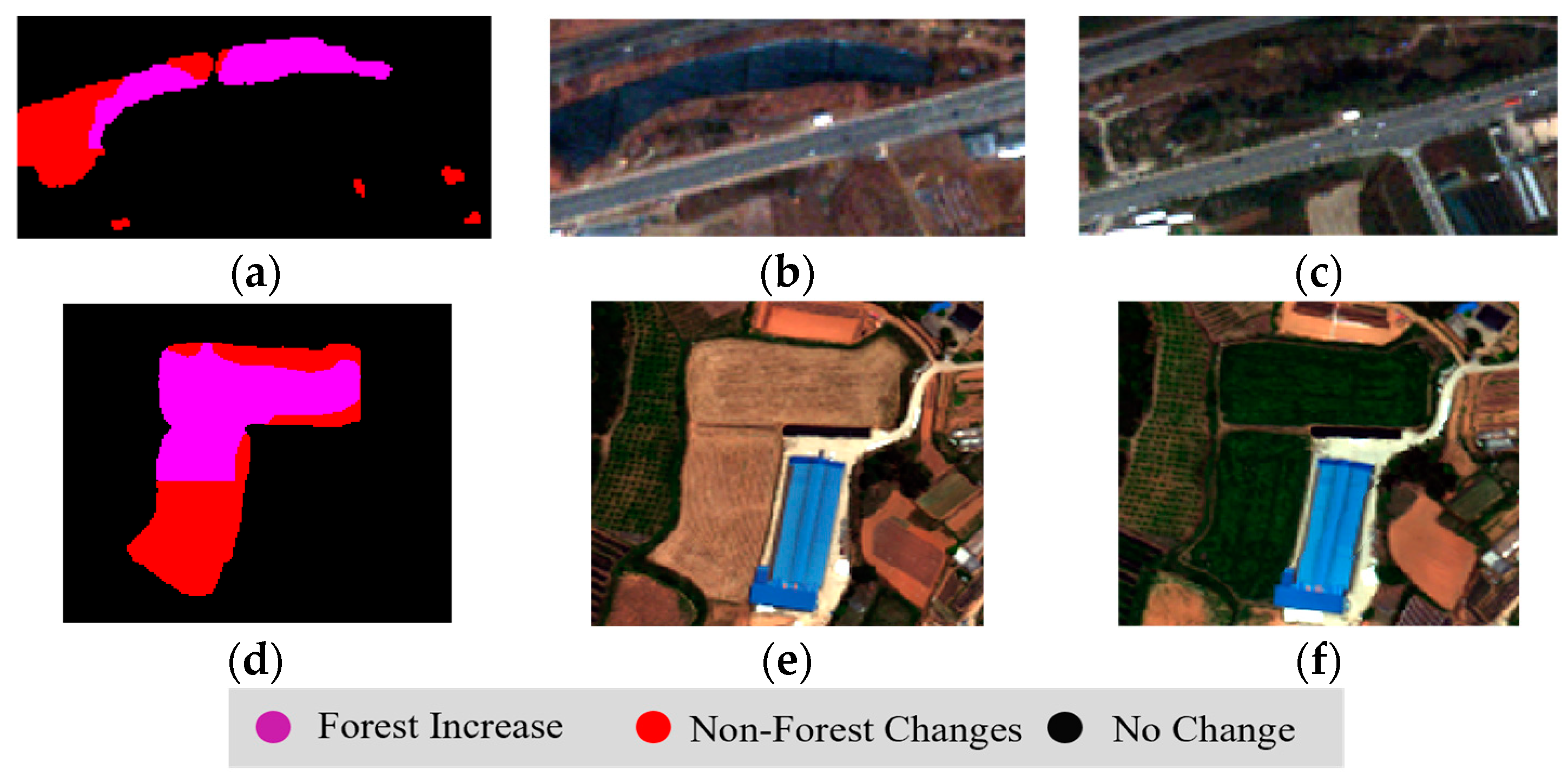
4.3. Finalizing Forest Cover Changes

After generating all the binary masks, they were concatenated in order to generate semantic change results for each site focusing on forest changes. This process helps in minimizing noise as well as falsely detected forest change regions. The semantic change map and reference maps were generated firstly by adding the predicted results and label images for extracting forest change regions from the binary forest masks. Then, these forest change regions were concatenated with the change mask for the final result.

In order to show the effectiveness of the proposed method, we compared the results generated via the proposed method with an unsupervised deforestation detection technique [13]. To this end, the unsupervised deforestation detection technique was used to generate the deforestation masks (i.e., forest decrease masks) while the forest increase mask was generated by swapping the bitemporal images. However, the technique is mainly developed for middle- to low-resolution satellite imagery and due to the use of VHR imagery the final forest change masks suffered from falsely detected regions and a copious amount of salt and pepper noise. Therefore, for effective comparison, we utilized the masks with the change masks generated in the proposed study. The final semantic change maps generated via the proposed methodology, semantic change maps generated after the utilization of the change mask with forest decrease and increase masks using the unsupervised deforestation detection technique, are shown in Figure 11 together with the semantic change reference maps. In Figure 11, the yellow color indicates a decrease in forest cover, purple is an increase in forest cover, red is non-forest changes, white is falsely detected or falsely labeled forest changes, and black is a no-change region.

It can be seen that the proposed method effectively detected decreased forest cover with a small number of false detections and missed detections in all three sites (i.e., Figure 11b,e,h) compared to the reference data (i.e., Figure 11c,f,i). Furthermore, undetected change regions were present in the binary change mask used in the proposed study; however, since our focus is forest cover CD, it is obvious from the figures that these undetected change regions have a subtle impact on forest cover CD and can thus be ignored. Moreover, due to the higher MR of the post-change binary forest mask compared to that of the pre-change binary forest mask generated via the proposed method and a minute amount of increase in forest cover, it remained undetected or falsely detected via the proposed method in Site 1. On the other hand, while using the unsupervised deforestation detection technique together with a change mask, numerous non-forest related changes were detected as decreased forest regions (i.e., shown by a yellow color in Figure 11a,d,g). Similarly, the increased forest regions were either missed or falsely detected by unsupervised deforestation detection technique in Sites 1 and 3.

After the generation of semantic change maps, forest changes concerning overall changes in the scenes were determined. The percentage of change in the overall scene of Site 1 was around 16.736% in the results predicted via the proposed method, whereas in the reference map it was around 15.64%. Moreover, in the results predicted via the proposed method, the total decrease in the forest cover compared to overall changes was around 13.617% and the calculated increase was 1.034%. In the reference map, these values were 15.74% and 2.49%. Due to the higher MR of the post-change forest cover map and lower percentage, the percentage of increase in the proposed study in Site 1 was considered to be an inaccurate result. Moreover, the percentage of decrease in the predicted results was higher than that in the reference map because in some regions the non-forest changes were detected as forest decreased regions. On the other hand, it is worth noting that the results obtained through the unsupervised deforestation detection technique displayed a significantly different pattern. Here, the percentages of decrease and increase in forest cover compared to overall changes were approximately 43.99% and 21.81%, respectively. This discrepancy can be attributed primarily to the numerous falsely detected forest change regions resulting from the use of VHR imagery.

Similarly, in Site 2, through the proposed method we observed that in 4 years around 3.5% of total change occurred in the full scene; 12.6% of total changes were related to a decrease in the forest cover whereas 1.43% were related to an increase in the forest cover. In the overall scene of Site 3, 5.63% of changes occurred in 1 year. Out of the total changes, the decrease in forest cover was 8.21% while the increase in forest cover was 1.25%. In Site 2 and 3, the forest cover increase was detected with less falsely detected forest increase regions compared to those in the results generated for Site 1, while for the results generated through the unsupervised deforestation detection technique for Sites 2 and 3, the decrease in forest cover was around 50.03% and 43.99% of overall changes. The increase in forest cover in Site 3 was shown to be 21.81% and in Site 2 it was not detected via the aforementioned method.

5. Discussion

Traditional CD methods that perform direct CD between binary forest masks will result in an increase in the number of incorrectly identified forest change covers. The proposed methodology accurately detected the decreased regions of forest cover in Site 1, Site 2, and Site 3 with a lower amount of missed and falsely detected regions. The non-forest change regions, however, contained an inadequate amount of miss detections, but since our study is focused on detecting changes in forest cover, these missed detections or false detections can be disregarded. Figure 12 shows a close-up view of regions of interest (ROIs) from the results predicted via the proposed method together with pre- and post-change images of the same ROIs from each site.

As mentioned earlier, in Site 1 due to the low percentage of increase in forest cover as well as the higher MR of the post-change forest cover map, the detected increased forest cover regions are considered to be inaccurate. A close-up view of the forest cover increase detected via the proposed method in a ROI from Site 1 is shown in Figure 13 in which the changes occur from a built-up region to agricultural land or from agricultural land to bare soil. In sites 2 and 3, the proposed method effectively detected the increased forest regions provided in Figure 14. In Site 3, as shown in Figure 14d–f, although it detected the increase, half of the forest change region in the close-up view was detected as a non-forest changed region.

6. Conclusions

In this study, we proposed a semantic CD technique while focusing on urban forest changes along with other urban changes. To this end, two networks, DeepLabv3+ for binary forest mask generation and DSIFN for binary change detection, were utilized and trained independently on open-source datasets. Then, transfer learning was performed using the dataset generated from VHR bitemporal images acquired via two different satellite images with different spatial resolutions. Then, the results generated by each network were concatenated for generating a semantic change result. To carry out the experiments, full scene tests were performed using the VHR bitemporal imagery of three urban cities acquired via three different satellites. The binary forest masks, generated via the proposed method from pre- and post-change images, showed a higher F1-score, kappa, IoU, and accuracy compared with the results generated via the NDVI, Unet, and SegNet. The final semantic change results showed that the proposed method can detect the changes in forest cover along with other urban changes. Moreover, the results showed that with the changes in the urban environment forest covers are changing considerably. Overall, in sites 1, 2 and 3, changes of 16.73%, 3.5%, and 5.63% occurred, in which 13.61%, 12.6%, and 8.21% of the total changes were related to a decrease in the urban forest cover. The use of both pre- and post-change VHR images minimized salt-and-pepper noise in regions related to forest cover changes in the sematic change result.

The results showed that the proposed method can effectively detect the regions related to forest cover decrease. However, because the tendency of forest cover decrease is usually higher than that of forest cover increase, as well as in the bitemporal images used in this study the forest cover increase regions were too small, regions where the forest cover was decreased were detected more effectively than those where there was an increase in forest cover. The proposed method can be used for monitoring the impacts of climate change, rapid urbanization, and natural disasters on urban environments especially on urban forests, as well as relations between changes in urban environments and urban forests. Moreover, this study can be used for the planning and development of cities and map updating. In the future, we will integrate the two networks in order to minimize the use of the two networks and independent training. A complex dataset will be generated for a semantic CD task containing changes in the classes related to the urban environment (i.e., urban grass, urban forest, urban trees, and built-up regions). Furthermore, we will apply the proposed method to additional datasets related to forest cover increase regions acquired via different satellite sensors.

References

1. Chen, W.Y. Urban nature and urban ecosystem services. In Greening Cities: Forms and Functions; Springer: Singapore, 2017; pp. 181–199. [Google Scholar]
2. Elmqvist, T.; Setälä, H.; Handel, S.N.; van der Ploeg, S.; Aronson, J.; Blignaut, J.N.; Gómez-Baggethun, E.; Nowak, D.J.; Kronenberg, J.; de Groot, R. Benefits of restoring ecosystem services in urban areas. Curr. Opin. Environ. Sustain. 2015, 14, 101–108. [Google Scholar] [CrossRef]
3. Long, L.C.; D’Amico, V.; Frank, S.D. Urban forest fragments buffer trees from warming and pests. Sci. Total Environ. 2019, 658, 1523–1530. [Google Scholar] [CrossRef]
4. Li, X.; Chen, W.Y.; Sanesi, G.; Lafortezza, R. Remote sensing in urban forestry: Recent applications and future directions. Remote Sens. 2019, 11, 1144. [Google Scholar] [CrossRef]
5. Islam, K.; Sato, N. Deforestation, land conversion and illegal logging in Bangladesh: The case of the Sal (Shorea robusta) forests. iForest Biogeosci. For. 2012, 5, 171. [Google Scholar] [CrossRef]
6. Samset, B.H.; Fuglestvedt, J.S.; Lund, M.T. Delayed emergence of a global temperature response after emission mitigation. Nat. Commun. 2020, 11, 3261. [Google Scholar] [CrossRef]
7. Alzu’bi, A.; Alsmadi, L. Monitoring deforestation in Jordan using deep semantic segmentation with satellite imagery. Ecol. Inform. 2022, 70, 101745. [Google Scholar] [CrossRef]
8. Desclée, B.; Bogaert, P.; Defourny, P. Forest change detection by statistical object-based method. Remote Sens. Environ. 2006, 102, 1–11. [Google Scholar] [CrossRef]
9. Ayhan, B.; Kwan, C.; Budavari, B.; Kwan, L.; Lu, Y.; Perez, D.; Li, J.; Skarlatos, D.; Vlachos, M. Vegetation detection using deep learning and conventional methods. Remote Sens. 2020, 12, 2502. [Google Scholar] [CrossRef]
10. Shakya, A.K.; Ramola, A.; Vidyarthi, A. Exploration of Pixel-Based and Object-Based Change Detection Techniques by Analyzing ALOS PALSAR and LANDSAT Data. In Smart and Sustainable Intelligent Systems; Wiley: Hoboken, NJ, USA, 2021; pp. 229–244. [Google Scholar]
11. Afify, N.M.; El-Shirbeny, M.A.; El-Wesemy, A.F.; Nabil, M. Analyzing satellite data time-series for agricultural expansion and its water consumption in arid region: A case study of the Farafra oasis in Egypt’s Western Desert. Euro-Mediterr. J. Environ. Integr. 2023, 8, 129–142. [Google Scholar] [CrossRef]
12. Schultz, M.; Clevers, J.G.; Carter, S.; Verbesselt, J.; Avitabile, V.; Quang, H.V.; Herold, M. Performance of vegetation indices from Landsat time series in deforestation monitoring. Int. J. Appl. Earth Obs. Geoinf. 2016, 52, 318–327. [Google Scholar] [CrossRef]
13. Mohsenifar, A.; Mohammadzadeh, A.; Moghimi, A.; Salehi, B. A novel unsupervised forest change detection method based on the integration of a multiresolution singular value decomposition fusion and an edge-aware Markov Random Field algorithm. Int. J. Remote Sens. 2021, 42, 9376–9404. [Google Scholar] [CrossRef]
14. Stow, D. Geographic object-based image change analysis. In Handbook of Applied Spatial Analysis: Software Tools, Methods and Applications; Springer: Berlin/Heidelberg, Germany, 2009; pp. 565–582. [Google Scholar]
15. Gamanya, R.; De Maeyer, P.; De Dapper, M. Object-oriented change detection for the city of Harare, Zimbabwe. Expert Syst. Appl. 2009, 36, 571–588. [Google Scholar] [CrossRef]
16. Keyport, R.N.; Oommen, T.; Martha, T.R.; Sajinkumar, K.S.; Gierke, J.S. A comparative analysis of pixel-and object-based detection of landslides from very high-resolution images. Int. J. Appl. Earth Obs. Geoinf. 2018, 64, 1–11. [Google Scholar] [CrossRef]
17. Lu, P.; Qin, Y.; Li, Z.; Mondini, A.C.; Casagli, N. Landslide mapping from multi-sensor data through improved change detection-based Markov random field. Remote Sens. Environ. 2019, 231, 111235. [Google Scholar] [CrossRef]
18. Wu, L.; Li, Z.; Liu, X.; Zhu, L.; Tang, Y.; Zhang, B.; Xu, B.; Liu, M.; Meng, Y.; Liu, B. Multi-type forest change detection using BFAST and monthly landsat time series for monitoring spatiotemporal dynamics of forests in subtropical wetland. Remote Sens. 2020, 12, 341. [Google Scholar] [CrossRef]
19. Bergamasco, L.; Martinatti, L.; Bovolo, F.; Bruzzone, L. An unsupervised change detection technique based on a super-resolution convolutional autoencoder. In Proceedings of the IGARSS 2021, Brussels, Belgium, 11–16 July 2021; IEEE: Piscataway, NJ, USA, 2021; pp. 3337–3340. [Google Scholar]
20. Shafique, A.; Cao, G.; Khan, Z.; Asad, M.; Aslam, M. Deep learning-based change detection in remote sensing images: A review. Remote Sens. 2022, 14, 871. [Google Scholar] [CrossRef]
21. Hou, B.; Liu, Q.; Wang, H.; Wang, Y. From W-Net to CDGAN: Bitemporal change detection via deep learning techniques. IEEE Trans. Geosci. Remote Sens. 2019, 58, 1790–1802. [Google Scholar] [CrossRef]
22. Zhang, X.; He, L.; Qin, K.; Dang, Q.; Si, H.; Tang, X.; Jiao, L. SMD-Net: Siamese Multi-Scale Difference-Enhancement Network for Change Detection in Remote Sensing. Remote Sens. 2022, 14, 1580. [Google Scholar] [CrossRef]
23. Mou, L.; Bruzzone, L.; Zhu, X.X. Learning spectral-spatial-temporal features via a recurrent convolutional neural network for change detection in multispectral imagery. IEEE Trans. Geosci. Remote Sens. 2018, 57, 924–935. [Google Scholar] [CrossRef]
24. De Bem, P.P.; de Carvalho Junior, O.A.; Fontes Guimarães, R.; Trancoso Gomes, R.A. Change detection of deforestation in the Brazilian Amazon using landsat data and convolutional neural networks. Remote Sens. 2020, 12, 901. [Google Scholar] [CrossRef]
25. Khan, S.H.; He, X.; Porikli, F.; Bennamoun, M. Forest change detection in incomplete satellite images with deep neural networks. IEEE Trans. Geosci. Remote Sens. 2017, 55, 5407–5423. [Google Scholar] [CrossRef]
26. Sefrin, O.; Riese, F.M.; Keller, S. Deep learning for land cover change detection. Remote Sens. 2020, 13, 78. [Google Scholar] [CrossRef]
27. Isaienkov, K.; Yushchuk, M.; Khramtsov, V.; Seliverstov, O. Deep learning for regular change detection in Ukrainian forest ecosystem with sentinel-2. IEEE J. Sel. Top. Appl. Earth Obs. Remote Sens. 2020, 14, 364–376. [Google Scholar] [CrossRef]
28. Zulfiqar, A.; Ghaffar, M.M.; Shahzad, M.; Weis, C.; Malik, M.I.; Shafait, F.; Wehn, N. AI-ForestWatch: Semantic segmentation based end-to-end framework for forest estimation and change detection using multi-spectral remote sensing imagery. J. Appl. Remote Sens. 2021, 15, 024518. [Google Scholar] [CrossRef]
29. Khankeshizadeh, E.; Mohammadzadeh, A.; Moghimi, A.; Mohsenifar, A. FCD-R2U-net: Forest change detection in bi-temporal satellite images using the recurrent residual-based U-net. Earth Sci. Inform. 2022, 15, 2335–2347. [Google Scholar] [CrossRef]
30. Nguyen-Trong, K.; Tran-Xuan, H. Coastal forest cover change detection using satellite images and convolutional neural networks in Vietnam. IAES Int. J. Artif. Intell. 2022, 11, 930. [Google Scholar] [CrossRef]
31. Zhang, C.; Yue, P.; Tapete, D.; Jiang, L.; Shangguan, B.; Huang, L.; Liu, G. A deeply supervised image fusion network for change detection in high resolution bi-temporal remote sensing images. ISPRS J. Photogramm. Remote Sens. 2020, 166, 183–200. [Google Scholar] [CrossRef]
32. Chen, L.C.; Zhu, Y.; Papandreou, G.; Schroff, F.; Adam, H. Encoder-decoder with atrous separable convolution for semantic image segmentation. In Proceedings of the European Conference on Computer Vision (ECCV), Munich, Germany, 8–14 September 2018; pp. 801–818. [Google Scholar]
33. Liu, M.; Fu, B.; Fan, D.; Zuo, P.; Xie, S.; He, H.; Liu, L.; Huang, L.; Gao, E.; Zhao, M. Study on transfer learning ability for classifying marsh vegetation with multi-sensor images using DeepLabV3+ and HRNet deep learning algorithms. Int. J. Appl. Earth Obs. Geoinf. 2021, 103, 102531. [Google Scholar] [CrossRef]
34. da Silva Mendes, P.A.; Coimbra, A.P.; de Almeida, A.T. Vegetation classification using DeepLabv3+ and YOLOv5. In Proceedings of the ICRA 2022 Workshop in Innovation in Forestry Robotics: Research and Industry Adoption, Philadelphia, PA, USA, 23–27 May 2022. [Google Scholar]
35. Lee, K.; Wang, B.; Lee, S. Analysis of YOLOv5 and DeepLabv3+ Algorithms for Detecting Illegal Cultivation on Public Land: A Case Study of a Riverside in Korea. Int. J. Environ. Res. Public Health 2023, 20, 1770. [Google Scholar] [CrossRef]
36. Ayhan, B.; Kwan, C. Tree, shrub, and grass classification using only RGB images. Remote Sens. 2020, 12, 1333. [Google Scholar] [CrossRef]
37. Wang, Z.; Wang, J.; Yang, K.; Wang, L.; Su, F.; Chen, X. Semantic segmentation of high-resolution remote sensing images based on a class feature attention mechanism fused with Deeplabv3+. Comput. Geosci. 2022, 158, 104969. [Google Scholar] [CrossRef]
38. Sharifzadeh, S.; Tata, J.; Sharifzadeh, H.; Tan, B. Farm area segmentation in satellite images using deeplabv3+ neural networks. In Proceedings of the 8th International Conference on Data Management Technologies and Applications (DATA 2019), Prague, Czech Republic, 26–28 July 2019; Revised Selected Papers 8. Springer International Publishing: Berlin/Heidelberg, Germany, 2020; pp. 115–135. [Google Scholar]
39. Chen, L.C.; Papandreou, G.; Schroff, F.; Adam, H. Rethinking atrous convolution for semantic image segmentation. arXiv 2017, arXiv:1706.05587. [Google Scholar]
40. Daudt, R.C.; Le Saux, B.; Boulch, A.; Gousseau, Y. Multitask learning for large-scale semantic change detection. Comput. Vis. Image Underst. 2019, 187, 102783. [Google Scholar] [CrossRef]
41. Wang, J.; Zheng, Z.; Ma, A.; Lu, X.; Zhong, Y. LoveDA: A remote sensing land-cover dataset for domain adaptive semantic segmentation. arXiv 2021, arXiv:2110.08733. [Google Scholar]
42. Ronneberger, O.; Fischer, P.; Brox, T. U-net: Convolutional networks for biomedical image segmentation. In Proceedings of the 18th International Conference on Medical Image Computing and Computer-Assisted Intervention—MICCAI 2015, Munich, Germany, 5–9 October 2015; Proceedings, Part III 18. Springer International Publishing: Berlin/Heidelberg, Germany, 2015; pp. 234–241. [Google Scholar]
43. Badrinarayanan, V.; Kendall, A.; Cipolla, R. Segnet: A deep convolutional encoder-decoder architecture for image segmentation. IEEE Trans. Pattern Anal. Mach. Intell. 2017, 39, 2481–2495. [Google Scholar] [CrossRef]
Figure 1. VHR bitemporal imagery and binary forest labels: (a) pre- and (b) post-change images of Site 1, (c) pre- and (d) post-change images’ forest labels, (e) pre- and (f) post-change images of Site 2, (g) pre- and (h) post-change images’ forest labels, (i) pre- and (j) post-change images of Site 3, and (k) pre- and (l) post-change images’ forest labels.
Remotesensing 15 04285 g001
Figure 2. VHR bitemporal imagery CD labels: (a) Site 1, (b) Site 2, and (c) Site 3.
Remotesensing 15 04285 g002
Figure 3. Flowchart of the proposed method.
Remotesensing 15 04285 g003
Figure 4. Proposed urban forest detection procedure by using DeepLabv3+ [32].
Remotesensing 15 04285 g004
Figure 5. Proposed change detection procedure using DSIFN [31].
Remotesensing 15 04285 g005
Figure 6. Semantic change detection focusing on forest changes.
Remotesensing 15 04285 g006
Figure 7. Training and validation graphs for transfer learning of Deeplabv3+: (a) training loss, (b) training accuracy, (c) validation loss, and (d) validation accuracy.
Remotesensing 15 04285 g007
Figure 8. Training and validation graphs for transfer learning of DSIFN: (a) training loss, (b) training accuracy, (c) validation loss, and (d) validation accuracy.
Remotesensing 15 04285 g008
Figure 9. Binary forest masks of pre-change image of each site generated by using (a) the NDVI for Site 1, (b) proposed method for Site 1, (c) label of Site 1, (d) NDVI for Site 2, (e) proposed method for Site 2, (f) label of Site 2, (g) NDVI for Site 3, (h) proposed method for Site 3, and (i) label of Site 3.
Remotesensing 15 04285 g009
Figure 10. CD results and label images: (a,b) Site 1; (c,d) Site 2; (e,f) Site 3.
Remotesensing 15 04285 g010
Figure 11. Semantic CD results: (a) unsupervised deforestation detection, (b) proposed method and (c) reference data of Site 1; (d) unsupervised deforestation detection, (e) proposed method, and (f) reference data of Site 2; (g) unsupervised deforestation detection, (h) proposed method, and (i) reference data of Site 3.
Remotesensing 15 04285 g011
Figure 12. Region of interest indicating decrease in forest cover: (a) reference data, (b) proposed method, (c) pre-change image, and (d) post-change image of Site 1; (e) reference data, (f) proposed method, (g) pre-change image, and (h) post-change image of Site 2; (i) reference data, (j) proposed method, (k) pre-change image, and (l) post-change image of Site 3.
Remotesensing 15 04285 g012aRemotesensing 15 04285 g012b
Figure 13. A close-up view of detected forest increase in Site 1: (a) proposed method, (b) pre-change image, and (c) post-change image.
Remotesensing 15 04285 g013
Figure 14. A close-up view of detected forest increase in Site 2 and 3: (a) proposed method, (b) pre-change image, and (c) post-change image of Site 2; (d) proposed method, (e) pre-change image, and (f) post-change image of Site 3.
Remotesensing 15 04285 g014