Article

Learning-Based Optimization of Hyperspectral Band Selection for Classification

Department of Electrical and Computer Engineering, Mississippi State University, Starkville, MS 39759, USA
*
Author to whom correspondence should be addressed.
Remote Sens. 2023, 15(18), 4460; https://doi.org/10.3390/rs15184460
Submission received: 28 July 2023 / Revised: 6 September 2023 / Accepted: 8 September 2023 / Published: 10 September 2023
(This article belongs to the Section Remote Sensing Image Processing)

Abstract

:
Hyperspectral sensors acquire spectral responses from objects with a large number of narrow spectral bands. The large volume of data may be costly in terms of storage and computational requirements. In addition, hyperspectral data are often information-wise redundant. Band selection intends to overcome these limitations by selecting a small subset of spectral bands that provide more information or better performance for particular tasks. However, existing band selection techniques do not directly maximize the task-specific performance, but rather utilize hand-crafted metrics as a proxy to the final goal of performance improvement. In this paper, we propose a deep learning (DL) architecture composed of a constrained measurement learning network for band selection, followed by a classification network. The proposed joint DL architecture is trained in a data-driven manner to optimize the classification loss along band selection. In this way, the proposed network directly learns to select bands that enhance the classification performance. Our evaluation results with Indian Pines (IP) and the University of Pavia (UP) datasets show that the proposed constrained measurement learning-based band selection approach provides higher classification accuracy compared to the state-of-the-art supervised band selection methods for the same number of bands selected. The proposed method shows 89.08 % and 97.78 % overall accuracy scores for IP and UP respectively, being 1.34 % and 2.19 % higher than the second-best method.

1. Introduction

In many remote sensing applications, a hyperspectral image (HSI) provides significant and important spectral information on a given scene by representing the spectral reflectance as three-dimensional image tensors, where each pixel has a high spectral resolution with hundreds of narrow bands [1,2,3]. Despite providing a rich and differentiable description of remote objects, the high number of bands in an HSI makes the data volume very large for storage and computation. HSIs also inherit the ‘curse of dimensionality’ in classification for a low number of training samples. In addition, the high correlation among the adjacent HSI bands causes information redundancy. For overcoming these limitations, hyperspectral band selection (HBS) plays an essential role.
In HBS, the main goal is to select a subset of original bands to capture the most relevant information, either in general or for a specific task, by discarding the redundant bands. In contrast to the dimension reduction [4] and feature extraction methods [5], where all data are acquired first and then a small set of informative combined features are computed, the goal of HBS is to preserve the useful information in the original spectral channels by passing only a small number of selected bands. Particularly for the classification task, the objective of the proposed model, final accuracy depends heavily on selected bands [6,7]. Over the years, various HBS methods have been presented in the literature. A detailed review of these methods can be found in [7]. Selecting a subset of bands that will lead to the maximum classification accuracy is basically a combinatorial problem. Instead of directly tackling this problem, a typical solution is to define a proxy criterion for classification accuracy to rank or search bands and select the top-ranked bands. Spectral moments, mutual coherence, entropy, and information divergence are several of the criteria utilized to sort the bands for ranking-based approaches [8,9,10,11]. A group of techniques adopts various distance metrics, such as Euclidean, Bhattacharyya, spectral angle, etc., and searches for a subset that minimizes the relevant distances [12,13,14,15]. Clustering bands into several groups and selects representative bands from each cluster [16,17,18] or utilizes sparsity-based priors [19,20,21], and either of these schemes or a combination of these schemes [22] have also been used for HBS. In the majority of the existing HBS literature, various types of applied criteria are only related to the final classification task, and optimizing these metrics can only provide a suboptimal classification performance.
In this paper, we propose a learning-based data-driven deep learning (DL) architecture for joint band selection and classification, where the network architecture minimizes the entropy loss for enhanced classification accuracy and learns a constrained measurement mask to select the optimal bands jointly. The band channels to be selected are learned from the utilized dataset during joint training with the classification network. The novelty of the approach is to implement a constrained measurement network for learning a binary mask that implements the band selection process simultaneously with a classification network. For the learning-based optimization of HBS, we utilize a probability mask to generate an initial proxy HSI dataset with only selected bands that are fed into the deep neural network-based classification part. The classification model is a deep convolutional neural network (CNN) with six hidden convolutional layers and two fully connected layers, which generates the final classification score of the input HSI data; however, any classification network that takes a similar size input can be used with the proposed band selection method. From the classification loss in the pipeline, with the help of back-propagation, we jointly learn the binary mask that satisfies the constraint for a given number of bands and the parameters of the classification network, implementing the final task of classification from the selected bands. The proposed architecture is tested over publicly available datasets and compared with the state-of-the-art approaches in HBS [11,16,23,24,25,26,27]. Our experimental results show higher classification accuracy than the compared HBS techniques for the same number of selected bands.
The main contributions of this work are as follows:
  • We introduce a constrained measurement learning network that learns a binary mask for band selection.
  • The measurement learning network and the classification network are jointly learned to minimize the classification loss, leading to optimally selected bands directly for the classification task.
  • The number of selected bands is an additional constraint for the measurement learning network, and the proposed architecture can learn binary masks for any desired number of bands.
  • The proposed architecture is flexible enough to adapt a new classification network that takes selected bands as its input, meaning that any new back-propagation adaptable classification network that performs better compared to our proposed classification model can replace the classification part of the proposed architecture, leading to further improvements in the performance.
The rest of the paper is organized as follows. Section 2 presents a revision of the background. Section 3 presents the theoretical explanation and the implementation details of the proposed model for learning-based joint HBS and classification. Section 4 explains the utilized datasets in detail. Section 5 shows the experimental settings and results. Section 6 provides a thorough discussion based on the study and the evaluations, along with a discussion of future work. A concluding remark is drawn in Section 7.

Abbreviations

The commonly used abbreviations in the paper are listed here.
HSI: Hyperspectral Image
HBS: Hyperspectral Band Selection
DL: Deep Learning
CNN: Convolutional Neural Network
DNN: Deep Neural Network
SVM: Support Vector Machine
MI: Mutual Information
IP: Indian Pines Dataset
UP: University of Pavia Dataset
OCA: Overall Classification Accuracy
ACA: Average Classification Accuracy
KC: Kappa Coefficient
The abbreviations used for the methodologies appearing in the paper are listed below.
MVPCA: Maximum Variance Principal Component Ananlysis [11]
FDPC: Fast Density Peak-based Clustering [23]
WaluDI: Ward’s Linkage sSrategy Using Divergence [16]
ISSC: Improved Sparse Subspace Clustering [21]
S-AEIS: Segmented Autoencoding Band Selection [25]
MMCA: Minimum Misclassification Canonical Analysis [11]
MEAC: Minimum Estimation Abundance Covariance [28]
CM-CNN: Contribution Map-based Convolutional Neural Network [26]
BHCNN: Bandwise Independent Hard Thresholding Convolutional Neural network [27]
MLBS: Measurement Learning-Based Band Selection (the proposed method)

2. Background and Related Work

HBS techniques can be supervised or unsupervised and should be selected based on the availability of labeled samples when gauging a predefined searching criterion. On the other hand, according to the searching strategy, HBS can use sequential forward search, sequential backward search, or evolutionary methods. A detailed review of HBS approaches can be found in [7]. Here, we present existing HBS approaches in two main categories: supervised and unsupervised. We also summarize deep neural network-based measurement learning techniques in the literature.

2.1. Unsupervised Hyperspectral Band Selection

Unsupervised hyperspectral band selection methods learn a band selection pattern without outside direction, either by utilizing structural information from the electromagnetic spectrum or by statistical approaches. The unsupervised approaches are usually expected to perform worse on data-specific tasks on average compared to the supervised approaches due to their data-incognizant nature. Another issue is the relevancy of the information basis with respect to the application; the selected information criterion may not be related to the task, and thus, the selected bands may not perform better than the all-bands case. On the other hand, the band selection process does not require a lengthy training process and instead can be applied directly to the utilized dataset. Also, unsupervised methods do not require ground-truth labels in order to work; therefore, they can be applied to a non-labeled dataset.
The first notable application of HBS without using class information is Maximum Variance PCA (MVPCA) [11], which ranks and selects the bands with higher loading factors. The Fast Density Peak-Based Clustering (FDPC) [23] method finds the cluster centers as the distance between all pairwise bands to find the independent density peaks that correspond to the selected bands. The unsupervised methods are based on clustering partition bands to a set of clusters where the bands from each cluster are selected from the similarity measures. For example, WaluDI [16] used Ward’s linkage for maximizing and minimizing inter and intra-cluster variances, respectively, to find the hierarchical clusters to represent the optimal set of bands that are selected from similarity measures like mutual information (MI) and Kullback–Leibler divergence.
The similarity measures can be derived from the mean of the data [17] using a kernel approach [29], spectral partitioning [18], or affinity propagation [30] to form the clusters. Unsupervised approaches also select representative bands that can best represent the rest of the bands under a given constraint on self-representation. These methods range from formulating the representation problem [19,20] to sparse regression [31] or sparse matrix non-negative factorization [21]. Improved Sparse Subspace Clustering (ISSC) [21] finds the bands in an unsupervised manner based on the notion that hyperspectral data live on a small number of low-dimensional subspaces, and representative vectors from these subspaces provide the desired bands. Overall, these unsupervised methods give the leverage of satisfying classification accuracy without the need for a class label. DL-based approaches have also started to be used in unsupervised HBS. For example, [25] utilizes an autoencoder, where the feature maps in the learned autoencoding representations are segmented to find the most significant bands without class labels. The results show that the segmented autoencoding band selection (S-AEBS) produces better classification performance than the non-segmented one (AEBS) and provides high classification accuracy among unsupervised HBS approaches.

2.2. Supervised Hyperspectral Band Selection

A supervised HBS method utilizes existing known labels on a training dataset to adopt a model, criterion or score that is associated with classification performance. This approach allows the obscure features of the dataset to be employed; for this reason, the selected bands with a supervised method usually provide higher accuracy levels for the task compared to bands selected by an unsupervised method. However, one should also be careful about the limitation of supervised methods, such as the dependence of an annotated dataset and the overshooting problem that occurs when the training dataset is inadequate for representing general features.
Supervised HBS techniques can rank bands by a selection score and select the top bands. The Minimum Misclassification Canonical Analysis method (MMCA) [11] sorts bands based on Fisher’s discriminant function to reduce the misclassification error. The main advantage of these methods is that they are computationally efficient. But, they are suboptimal since they do not optimize the final classification directly. In order to find better sets of bands, the methods in [15,28] utilize an optimization criterion with the aid of prior information on the class spectral signature. In [15], the concept of the band add-on (BAO) algorithm was introduced to iteratively select bands that increase the angular separation between two classes of spectra based on the average distance and minimum distance methods. In [28], the Minimum Estimation Abundance Covariance (MEAC) algorithm was proposed to use the prior information of the class spectral signatures for selecting dissimilar bands incrementally via minimizing the trace of the inverse of the covariance matrix of the selected bands. In addition, supervised methods based on particle swarm optimization [32,33,34] and recursive elimination [35] update the searching strategy with improved optimization to find the best subset. The idea of linear representation is also used for HBS. With labeled samples, a sparse linear regression method was developed in [31], and discriminative bands were selected by ranking their contributions in the representation. Some supervised HBS techniques [36,37,38] include a classification step with a classifier, such as Support Vector Machine (SVM).
DL models have recently started to be used in hyperspectral image problems [39]. DL-based band selection approaches typically use a predefined implementation like embedded learning or classification to select the optimal bands. One notable approach uses a pre-trained CNN [40] to extract deep features as priors to an AdaBoost SVM classifier to select the most predominant bands. The work in [41] used a pre-trained CNN model where the band selection is carried out based on partitioning the subspace of distance density. HBS based on attention mappings is used in [42], where DL models produce more sophisticated feature maps for classification with the most informative sets of bands by optimizing the deep CNNs. In [26], contribution maps of each class were produced to record the discriminative band locations, which are progressively added to CNNs to select more distinguished bands. Recently, the work in [27] introduced the concept of band-independent convolution and hard thresholding (BHCNN) to select the bands for the classification task. BHCNN applies bandwise 1 × 1 convolution and the hard thresholding of weights based on the absolute values of the kernels to select and remove the bands before feeding them into the classification network. This method utilizes the straight-through estimator (STE) to approximate the gradient, and it optimizes the classification network that consists of 3D dilated convolutions to enable a scalable coarse-to-fine loss (Table 1).

2.3. Deep Neural Network-Based Measurement Learning
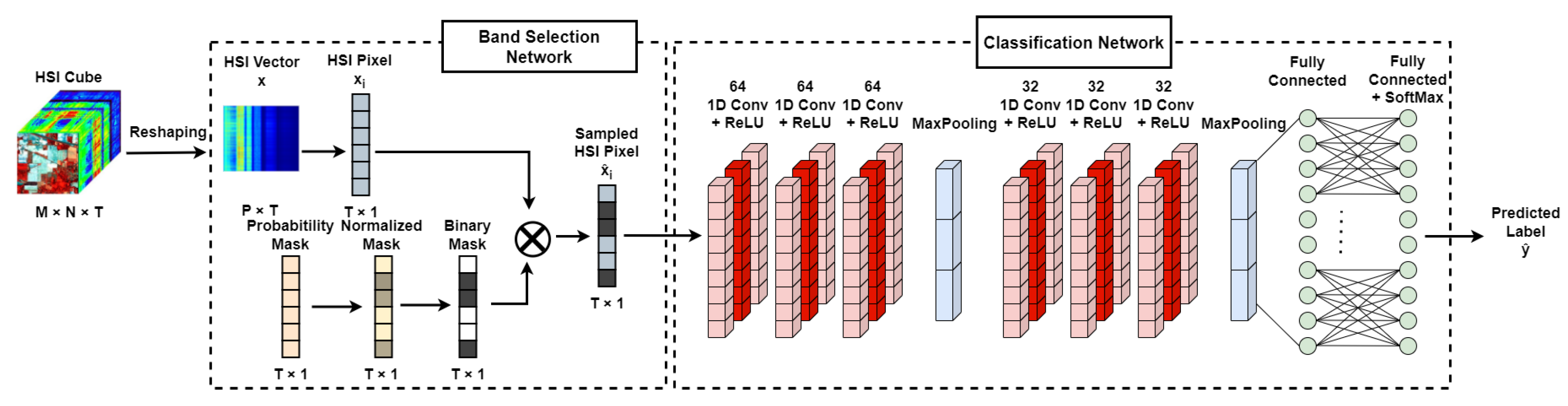
Measurement learning is the problem of learning a measurement pattern jointly for main tasks such as classification, detection, compression, or reconstruction. The joint measurement learning-classification approach usually requires a more complex design of the input–output stream and loss function, compared to applying band selection first and classification later. These models also usually require more parameters and operation at training, which increases complications in memory allocation, although usually, this is not an overwhelming issue. Compared to the complications in design and computation, the advantage of the joint approach is well worth it for the increase in performance compared to solving two separate problems.
Measurement learning has been recently studied with DL architectures mainly within the computational imaging and the sparse signal reconstruction framework [43,44,45,46,47,48]. These approaches use the advantage of the end-to-end training nature of deep neural networks (DNNs) to model the measurement process by a dense or convolutional layer to replicate the linear measurement process, starting from a fixed random Gaussian measurement matrix similar to the compressive sensing scenario [49,50,51]. It was shown that measurement matrices leading to enhanced reconstruction or classification performance can be learned; however, the learned measurement matrices are not constrained in the sense that they learn a linear combination of all available projections. This makes them unsuitable for applications such as HBS because the measurement for band selection is only a subset of the full spectral observation and not a linear combination of spectral observations. For HBS, a constrained measurement having only binary values needs to be learned. In [52], constrained measurement matrices are learned with binary or bipolar values by incorporating additional losses that force the desired constraint. In [53], a DL approach jointly learning measurement for classification was shown. The work in [27] shows a similar approach to measurement learning, focusing on reducing the number of bands through hard thresholding rather than through learning a measurement matrix.

3. Proposed Method

The proposed data-driven joint band selection and classification architecture can be decomposed into two concatenated networks: (1) a band selection network that identifies an optimal band selection pattern, and (2) a classification network that uses only selected bands to determine the output class. Figure 1 shows the proposed network architecture. The band selection network takes the full single-pixel spectral dataset as input and generates a band-selected proxy HSI spectrum. The proxy spectrum is produced by multiplying the input spectrum with a learned binary mask where the selected bands are represented by ones and the redundant bands are represented by zeros. The output of the band selection network is passed into a DNN-based classification network to obtain the final classification label of the given HSI pixel. The entire architecture comprising both the learned band selection and the classification networks is learned by minimizing the final classification loss; hence, learned band selection optimizes the final goal of classification directly. Since we employ a constrained measurement learning strategy to select the bands, the proposed approach is named Measurement Learning-based Band Selection (MLBS), and a detailed description of the architecture is provided next.

3.1. Learning-Based Optimization of Band Selection Pattern

The input of the band selection network is a spectral vector X of size T × 1 , where T is the total number of spectral bands as illustrated in Figure 1. The aim is to learn a binary mask that selects the optimal bands; however, discrete operations are not differentiable. To make the operation differentiable, we begin with an unconstrained vector V R T that will be the seed for the band selection process. This seed is initialized randomly from the normal distribution. These weights will be updated through the backpropagation process. With V as a parameter, we can construct a probabilistic mask S of size T × 1 , as shown in Figure 1. We want the probabilistic map S to be defined on the entire spectral space and at each spectral band, taking a non-negative continuous probability value between 0 and 1; thus, S [ 0 , 1 ] T . This can be achieved via the equation S = σ t ( V ) , where σ t ( . ) is the element-wise sigmoid function, and t is the slope of the sigmoid that acts as a hyperparameter. From this,
S i = σ t ( V i ) = 1 1 + e t V i ,
for the i-th spectral band. Since the value of S i lies in the region [ 0 , 1 ] , it describes a Bernoulli random variable for the i-th band. If we draw binary realizations from S , we get a binary mask B { 0 , 1 } T such that B i = 1 T β ( S i ) , where β ( s ) represents the Bernoulli random variable with parameter s. The obtained binary mask B will have a value of 1 for the bands that are selected and 0 for the bands that will not be selected.
Let us assume we have a labeled hyperspectral dataset with full spectral observations { X j R T } j = 1 N , where N is the total number of hyperspectral data samples and each sample is a T × 1 spectral vector. Since binary realizations drawn from S define the binary mask B , we would like to minimize the classification loss in the expected sense. Hence, we aim to solve the following optimization problem:
arg min V , Θ E B i = 1 T β σ t ( V i ) j = 1 N L ( f Θ ( B X j ) , j ) s . t . 1 T σ t ( V ) 1 = α ,
where f Θ is the mapping for the classification network with learnable parameters Θ , B X j is the classification network input with ⊙ being the pointwise multiplication, and L ( f Θ ( B X j ) , j ) refers to the cross-entropy loss between the predicted network output and the ground truth j . The α value denotes the ratio of the selected bands. The constraint 1 T σ t ( V ) 1 = 1 T S 1 = α ensures that the probabilistic mask has on average α number of non-zero elements.
The optimization problem in (2) includes an expectation over realizations from the probabilistic map. To implement the minimization, we can obtain an approximation of the expectation by Monte-Carlo averaging for K independent trials:
arg min V , Θ 1 K k = 1 K j = 1 N L ( f Θ ( b ( k ) X j ) , j ) s . t . 1 T σ t ( V ) 1 = α ,
where b ( k ) are independent realizations drawn from the distribution i = 1 T β ( S i ) . The minimization in (3) takes the same form of variational autoencoder (VAE) in [54], where the authors use the re-parameterization trick to rewrite b ( k ) = U ( k ) σ t ( V ) . Here, U ( k ) deduces the independent identical realizations from i = 1 T u ( 0 , 1 ) , which is a set of random uniform variables between [ 0 , 1 ] . Thus, if the inequality is satisfied, then the result of this inequality would be 1; otherwise, it is 0, leading to a binary mask realization. Although the inequality operation provides a binary mask, it does not allow end-to-end learning in this form since the thresholding function is non-differentiable. To make the total loss function for the HBS and classification differentiable, we relax the thresholding operation with another element-wise sigmoid function σ r with slope r similar to [55,56]. Then, the loss minimization problem becomes
arg min V , Θ 1 K k = 1 K j = 1 N L ( f Θ ( σ r ( σ t ( V ) U ( k ) ) X j ) , j ) s . t . 1 T σ t ( V ) 1 = α .
The optimization in (4) is still a constrained minimization problem, imposing the number of selected bands. To convert (4) to an unconstrained optimization, we utilize a normalization layer defined as
N α ( S ) = α s ¯ S if s ¯ α 1 1 α 1 s ¯ ( 1 S ) otherwise
where the parameter s ¯ is the average of the pre-normalization of probability mask S , defined as s ¯ = S 1 / T . It can be seen that the values of N α ( S ) [ 0 , 1 ] T and satisfy the constraint N α ( S ) 1 = T α . The normalized mask computed from the probability mask is shown in Figure 1. Using the normalization layer output, the final objective function can be rewritten as
arg min V , Θ 1 K k = 1 K j = 1 N L ( f Θ ( σ r ( N α ( σ t ( V ) ) U ( k ) ) X j ) , j )
Minimizing (6) through back-propagation will produce the parameters of the classification network Θ and the seed vector V for the probabilistic mask jointly. The probability mask S is generated by using an element-wise sigmoid with slope s on V , and it is rescaled through the norm layer. The output of the norm layer is passed into another element-wise sigmoid with slope r to produce the binary mask B = σ r ( N α ( S ) U ( k ) ) . Once B is obtained, the selected band X j ^ can be obtained as the element-wise multiplication of the binary mask B and X j . The selected bands are then fed into the classification network part, as shown in Figure 1, which is detailed next.

3.2. Classification Network

The second part of the proposed MLBS algorithm is the classification network, the visualization of which can be found on the right-hand side of Figure 1. The classification network takes the band-selected data as the input and gives the class prediction of the given pixel label j as the output. Our goal in this study is to demonstrate a joint band selection and classification scheme, and for the latter task, we opt to use a deep convolutional neural network (CNN) learning feature hierarchically from the selected bands due to the proven performance of convolutional layers and deep structures for learning features directly from the data in many classification tasks, especially in computer vision applications [57]. Kernel sizes and numbers, on the other hand, were chosen heuristically to trade-off between the computational time and the accuracy. The proposed framework also allows one to utilize any other existing DNN-based classification architecture with similar inputs and outputs the classification network to further optimize classification performance.
In the proposed architecture, the main building blocks are 1 D convolutional filters (Conv1D), followed by ReLU activation functions, as illustrated in Figure 1. The first convolutional block consists of three Conv1D and ReLU pairs, and each Conv1D layer uses 64 filters with a stride of 1 and a kernel length of 3. With the same stride, kernel length, and activation value, the Conv1D layers in the second convolution block have 32 filters. After each Conv1D block, a max-pooling layer (Maxpool1D) comes in order to downsample the extracted features with a pooling size of 2. The output of the second convolutional block is flattened before being fed into a set of fully connected dense layers. The first dense layer consists of 25 output neurons with ReLU activation, while the second layer generates class labels for the given HSI data. The output of the second layer passes through the SoftMax function as an activation function, converting the output into the class probabilities of the input HSI pixel. The classification loss function L ( j ^ , j ) of the j th spectral sample is the cross-entropy loss, which is defined as
L ( j ^ , j ) = c = 1 C j , c l o g ( j , c ^ ) .
where ^ j , c is the SoftMax layer output that gives the probability of the j th sample belonging to c th class, and j ^ and j represent predicted and ground truth logits, respectively. Once we have the prediction of the probabilities of all class labels, the final class label is declared as the one that corresponds to the maximum class probability, i.e., y j ^ = arg max c j , c ^ . The total loss function is back-propagated to learn both the band selection and the classification network parameters jointly. The overall steps of MLBS for joint band selection and HSI image classification can be summarized in Algorithm 1.
Algorithm 1 MLBS Algorithm
Input: 
Selection Ratio α , Input HSI Data of size N × T , slopes for sigmoid t and r, Mini-batch size B, Number of Epoch E
Output: 
Trained parameters V ^ , Θ ^
  1:
for  e = 1 : E  do
  2:
    for  b = 1 : B  do
  3:
        Apply Equation (1) with slope t to find the random mask S
  4:
        Apply Equation (5) to generate the normalized mask N α ( S )
  5:
        Apply σ r to generate the binary mask B
  6:
        Apply X j B to select bands
  7:
        Compute classification network output
  8:
        Compute loss L in Equation (7) for the minibatch
  9:
    end for
10:
    Update V ^ , Θ ^ using backpropagation
11:
end for

4. Datasets

In this work, we opt to use two publicly available HSI datasets: the Indian Pines (IP) [58] and the University of Pavia (UP) [59].
The IP dataset was collected in a test site in Northwest Tippecanoe County, Indiana, located 6 mi west of West Lafayette via an Airborne Visible/Infrared Imaging Spectrometer (AVIRIS). The image covers a 2 × 2 mile agricultural area with 20 m spatial resolution. It has a spectral resolution of 10 nm that covers a range from 200 to 2400 nm. Initially, the collected HSI data had dimensions of 145 × 145 × 224 , where 224 denotes the total number of spectral bands. Purdue University initially reduced the number of bands to 220 for radiometric corrections, while the Computational Intelligence Group (CIG) further reduced it to 200 by eliminating bands that were corrupted due to water absorption. The HSI data contain a total of 10 , 249 labeled samples for a total of 16 classes that include alfalfa, no-till corn 1, minimal-till corn, corn, grass/pasture, grass/trees, mowed grass/pasture, windowed hay, oats, no-till soybeans, minimal-till soybeans, clean soybeans, wheat, woods, building/grass/tree drives, and stone/steel towers.
For the UP dataset, a reflective optics spectrographic imaging system (ROSIS)-3 sensor collected a hyperspectral image of a protion of Pavia city in Italy with 115 bands within the spectral range from 0.43 to 0.86 μm in the University of Pavia area. The spatial resolution is 1.3 m. In this paper, we use 103 bands after removing the bands with low SNR values. The data tensor size is 640 × 340 × 103. The UP data are divided into 9 classes with a total of 42 , 776 labeled samples, including asphalt, meadows, gravel, trees, painted metal sheets, bare soil, bitumen, self-blocking bricks, and shadows. The ground truth images for both datasets can be found in the first column of Figures 5a and 6a.

5. Experimental Results

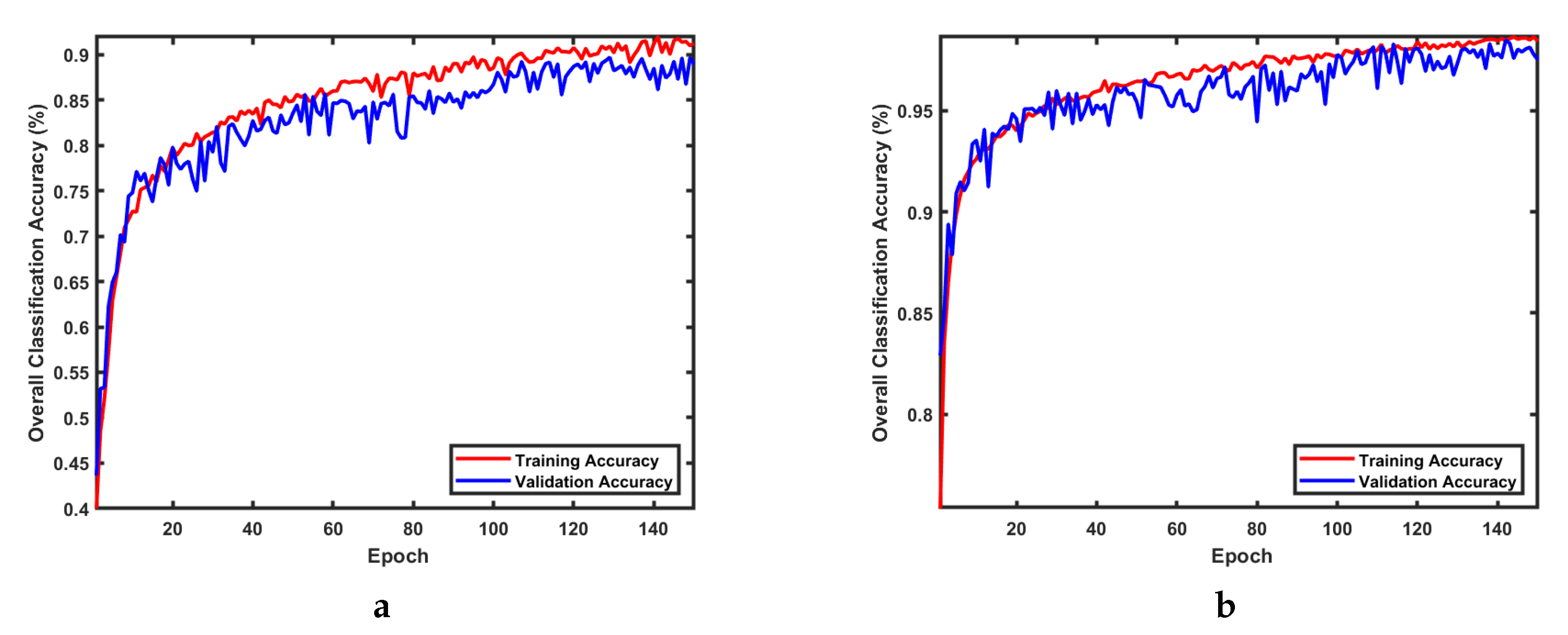
5.1. Experimental Setup

The training process follows a 10/90 percent split. For both datasets, only randomly selected 10 % portion of data points belonging to each class are allocated as the training dataset. The rest of the data points are used to form the test dataset. This is exactly the same dataset split followed in the compared studies. Both datasets are also normalized to the interval [ 0 , 1 ] with respect to the lowest and highest brightness values.
The implementation details of the training procedure for the MLBS model are described as follows: The slope values for the first and second sigmoid functions in Equation (6) are chosen as t = 5 and r = 200 . These values are selected based on a heuristic grid search. For the training of the MLBS architecture, the gradient descent based on the Adaptive Moment Estimation (ADAM) optimizer is used with a batch size of 16. Varying learning rates from 0.1 to 0.0001 were tested to find the best learning rate value heuristically. In the end, the models were trained with a decreasing learning rate from 0.01 in the first 50 epochs to 0.001 for the next 50, and finally, 0.0001 for 50 more epochs. The model is therefore trained for 150 epochs in total.
The model implementation, training, and evaluation codes were written in Python language using the TensorFlow library and the Keras API. Figures were drawn with matplotlib library, and SciKit’s metrics library was used for evaluation. The training and evaluation codes were processed in a dedicated server with 3 NVIDIA Titan RTX GPUs. The implementation of the MLBS model with datasets and the source code can be found in the link [60].

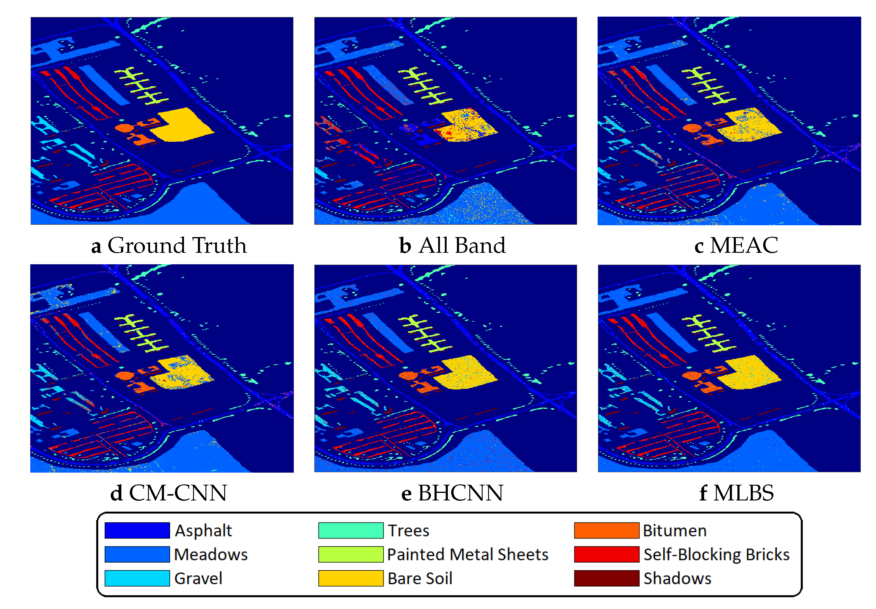
5.2. Joint Band Selection and Classification with MLBS

We first demonstrate the performance of MLBS for the case where the binary mask selects 30 bands. The learning curves over different epochs are shown in Figure 2, which illustrates the overall training and test classification accuracy over 150 epochs. The figures for both datasets clearly show that classification accuracy increases as training progresses. Learning curve plots also show very close training and validation accuracy values, indicating that the MLBS approach is not overfitting.
The binary mask over different epochs as learning progresses over the training data is also visualized in Figure 3 for both IP and UP datasets, together with the average classification accuracy values corresponding to the dataset and the epoch. The figure shows that the initial binary mask in the first epoch expectedly produces a low classification accuracy for both datasets. The weights for the binary mask are initialized randomly from the normal distribution satisfying the selected number of band constraints. As the learning progresses with increasing epoch numbers, better band selections are obtained, which in turn leads to higher classification performances. For example, for the IP dataset, while the initial band selection provided an accuracy of 44 % , after 10 epochs with updated band selections, this increased to 75 % . At 100 epochs, an accuracy of 88 % is achieved, and more stable changes are observed after 100 epochs. A similar trend can be observed in the UP dataset. In the first epoch, the average accuracy starts at 83 % , and just after 10 epochs, the accuracy level approaches 93 % . At the end of the training, the accuracy level reaches 95 % . Another important point is that the selected bands are randomly spread or connected in the earlier epochs; as the training progresses, selected bands are more clustered in certain spectral ranges that are useful for class separation, but many selected bands are not adjacent, which means they are less correlated.
Figure 3 also shows that in the first epoch, the condition in Equation (5) roughly satisfies the selected ratio of selected bands with the randomly initialized weights, but as the training progresses, the number of selected bands converges to the chosen ratio—in this case, 30 bands. Overall, Figure 2 and Figure 3 together show the effectiveness of the data-driven manner for the HBS problem, jointly enhancing the classification performance. The MLBS model reaches a higher overall classification performance for both datasets during training and provides a transparent framework for a post-training analysis of the selected bands.

5.3. Quantitative Analysis and Comparisons

The next analysis is the quantitative comparison of the proposed MLBS model with various state-of-the-art HBS techniques for both datasets as a function of the number of selected bands in terms of classification performance. The MLBS is a supervised technique, where we train the proposed joint band selection and classification neural network utilizing the training dataset described earlier. For a fair comparison, the proposed approach is compared with state-of-the-art supervised techniques such as MEAC [28], BHCNN [27], and CMCNN [26]. While MEAC is a signal processing-based technique, BHCNN and CMCNN are deep neural network-based approaches like MLBS. These methods are selected for comparison because they provide the state-of-the-art available classification performance according to their respective publications and reviews, such as [7]. In addition, there are many unsupervised techniques, and the classification accuracies of the high-performing ones like FDPC [23], WaluDI [16], ISSC [21], and S-AEBS [25] are already given in [7]. Here, we focus on the comparison of the supervised techniques, wherein we implemented each of the compared approaches and achieved the classification results in the same machine.
All the compared techniques were tested over the same two publicly available HSI datasets discussed in Section 4. For quantitative comparisons, we use the overall accuracy (OCA), average accuracy (ACA), and kappa statistics (KC) metrics as defined in [61]. OCA is defined as the ratio of the total number of correctly classified testing samples to the total number of testing samples. ACA metric shows the average classification accuracy for all class labels. And finally, KC measures the agreement between the classification results and the ground truth.
The OCA of all compared approaches is shown in Figure 4 as a function of the number of selected bands varying from 5 to 60 with an increment of 5. The OCA achieved using all the available bands is shown on the same plots as a red-stripped line. All of the compared approaches use the same classification network architecture, and hence the observed performance differences, are expected to be due to different band selection approaches. From Figure 4, it is clear that the proposed MLBS approach outperforms compared state-of-the-art approaches in both datasets, providing higher OCA over all the tested number of band cases. MLBS provides approximately 3 % more accuracy for the IP dataset and 2 % more for the UP dataset than the next performing approach. This enhanced performance is due to the design of the MLBS, which directly minimizes the classification loss while learning to select the bands and implement classification jointly. BHCNN, which is also a DL-based approach, provides the overall second-highest classification accuracy compared to other techniques.
Figure 4 shows the change in classification accuracy with respect to the available number of selected bands for all the compared algorithms. The accuracy of MLBS gets higher compared to the all-bands case only when the selected number of channels is more than 10. It can also be observed that as more bands are selected, the OCA for all approaches increase, and after the number of selected bands exceeds 30, the change in the OCA performance of the MLBS and the compared techniques mostly flattens. MLBS is seen to outperform the compared techniques for both low or high numbers of selected band regimes.
The OCA metric shows the overall accuracy. In order to show a more detailed classification performance of each class, as well as the ACA and KC metrics, the performance of the MLBS model along with the compared algorithms for 30 selected bands with both the IP and the UP datasets are listed in Table 2 and Table 3, respectively. Each row shows the classification performance for the specified classes, as well as the average metrics of ACA, OCA, and KC for the compared techniques and when using all the bands. The highest performance for each row is indicated in bold. The proposed MLBS model can distinguish individual labels more clearly compared to other algorithms for most of the cases, as it did for OCA. For both the IP and UP datasets, MLBS gives the highest classification accuracy for most of the individual classes, while for several classes, BHCNN is the top-performing approach. The overall highest score in most individual classes indicates MLBS as achieving the highest ACA and OCA results for both datasets; that is, 89.08 % and 97.78 % OCA and 82.88 % and 93.77 % ACA for the IP and UP datasets, respectively. For the KC metric, while MLBS is the outperforming approach for the IP dataset with a score of 81.14 % , BHCNN is the top-performing technique for the UP dataset with a score of 93.55 % . It should be noted that the two DL-based joint band selection and classification techniques provide the highest performances, indicating the benefit of data-driven DL approaches for band selection. Since the same classification network is utilized for all compared techniques, the differences between techniques are mainly due to the different band-selection schemes.
For the visualization of the classification results, the classification labels of both datasets as color maps, along with the color maps of the predictions of all compared methods, are shown in Figure 5 and Figure 6. The classification maps of the DL-based methods (CM-CNN, BHCNN and MLBS) for the 30 selected band case are illustrated in the bottom rows. The sixteen classes of ground objects in Figure 5a for the IP dataset and the nine classes of objects in Figure 6a for the UP dataset are detailed in Table 2 and Table 3, respectively. The classification maps produced by both the proposed MLBS and the BHCNN techniques are very close to the ground truth images, with MLBS showing slightly better performance. Since classifications are performed for each spatial pixel, misclassifications at the pixel level can be seen for all compared techniques and for both datasets.

5.4. Computational Analysis

A final analysis shows the performance of MLBS and the compared band selection models in terms of computational time. For supervised techniques such as MLBS or the compared approaches, there are two categories of computation. First, the models are trained over the training dataset with an offline learning process, and later, the inference on a sample test dataset can be achieved with the trained model. Here, we provide both the training and the inference computational times for the compared approaches.
Table 4 presents the training and inference times of the compared techniques under both datasets. All approaches were trained and evaluated on the same computer, which has 3 NVIDIA Titan RTX GPUs, and the computational time values were collected during the training and inference processes. The total number of trainable parameters in the final MLBS model is counted as 212,954 for the IP dataset and takes 2.79 MB in memory, while the MLBS model for the UP dataset has 188,050 parameters and takes 2.48 MB in memory.
With the dataset training setup detailed in Section 5.1, the training with the whole IP dataset takes approximately 1216 s for the MLBS approach, while the inference time for an individual test sample is 0.0937 s on average. For the UP dataset, the computational time for training takes 5050 s, and the average inference time is 0.1249 s for an individual test sample.
In general, the overall training time for the DL-based methods are much higher compared to the testing time. It should be noted that the time used for training MLBS and other DL-based band selection models is related to the model size, model hyperparameters, and dataset dimensions. Although high, the training for DL-based approaches should be conducted once, and when trained, the same model can be used for testing; the inference times listed in Table 4 indicate the testing computational complexity for testing. Compared approaches show varying training and inference times depending on the overall complexity, but usually, the training and inference times are generally similar; while slightly higher, the training time for BHCNN and the inference time for CM-CNN are observed. The proposed MLBS has an average computational complexity across the compared techniques.

6. Discussion and Future Work

In this work, a DL-based architecture that is composed of a band selection network followed by a classification architecture is trained jointly to optimize the final classification. In this way, the proposed network learns to select the bands that will optimize the classification performance. The evaluation of the proposed MLBS approach on two test datasets shows enhanced classification performance for the same number of selected bands. Nevertheless, there are several points to consider in the implementation of MLBS in order to prepare a roadmap for future work. In this section, we discuss several points for improvement and various directions for future work.
The first important point is that MLBS is a supervised neural network model that needs to be trained. Hence, annotated, clean, high-quality, and diverse training data are needed to train the model that can be generalizable for various cases. Our results evaluate MLBS over two publicly available hyperspectral datasets; however, further developments related to annotated datasets, such as those in [62], will benefit DL-based techniques such as MLBS. In addition, the IP and UP datasets used in this study have different bandwidths, number of bands, image size, resolution, and segmentation classes; this prevents them from being used together simultaneously. Instead, evaluations within each dataset are made. Datasets that are compatible with each other will enhance DL-based techniques and provide better evaluations against the generalization of the DL models.
A tangential problem to the first issue concerns the nature of the datasets. Both the IP and UP datasets used in this study have different bandwidths, number of bands, image sizes and resolution and segmentation classes; by themselves, they are not adequately numerous datasets for ML solutions. These differences prevent them from being used together at once; rather, only one dataset can be used for a single evaluation. Making the available datasets compatible to provide consistency between them will be beneficial work for better DL-based HSI band selection models.
The second important point is the lack of interpretability of the general neural network-based models. MLBS is a neural network model, and as most other neural networks, the internal decision process of why the model prefers certain bands against others is almost completely unclear to an observer. While this is a more general limitation for major DL-based approaches, more interpretable models and physical explanations related to some selections are desired for understanding the selection process and the advantages of the selected bands. We plan to add more interpretability to the next iteration of the MLBS model, and we plan to make it more physics-aware by adding prior physical information by updating the loss function. Physics-informed NN algorithms applied in different problems shed light on this discussion [63].
The third point is that MLBS provides a general framework for band selection and classification. MLBS is composed of two networks following each other, and one can select a different classifier and jointly learn the band selection and classification scheme as long as the classifier is learnable, in the sense that we should be able to apply back-propagation through the classifier. This allows for the optimization of the classification network so that the joint architecture can provide enhanced band selection and classification performance. Currently, the MLBS approach uses a classical convolutional network structure for classification. While this study focuses on the band selection model, for future work, we plan to design and compare different classification networks to optimize the joint performance. One current trend in this respect seems to be combining signal compression with autoencoder-based architectures for more efficient classification and dimensionality reduction embedded in the architecture [64,65,66]. There are also architectures based on attention maps for better feature extraction [67,68]. Such enhancements on the classification part of the model have the potential to lead to higher joint performance.

7. Conclusions

In this work, a deep neural network-based learning model is proposed to select bands from the hyperspectral data. The proposed architecture is composed of a constrained measurement learning network for band selection, followed by a convolutional network for classification. The combined architecture is jointly trained to minimize the classification loss learning to select the bands that will directly enhance the classification performance. The architecture is flexible to adapt any superior DL-based classification model that can lead to enhanced band selection and classification performance.
The proposed MLBS approach has been evaluated with Indian Pines (IP) and the University of Pavia (UP) datasets. It is observed that the proposed approach results in higher classification accuracy compared to the existing state-of-the-art supervised band selection methods for the same number of bands selected. In the case of the 30 selected bands, MLBS achieves ACA and OCA scores in both the IP (89.08% OCA and 82.88% ACA) and UP (97.78% OCA and 93.77% ACA) datasets. Computational analysis indicates that the proposed technique has similar computational complexity to compared approaches for both training and inference.

Author Contributions

Conceptualization: A.C.G.; methodology: R.M., C.O.A. and A.C.G.; software: R.M. and C.O.A.; validation: R.M., C.O.A. and A.C.G.; formal analysis: R.M. and C.O.A.; investigation: R.M., C.O.A. and A.C.G.; resources: A.C.G.; data curation: R.M. and C.O.A.; writing—original draft preparation: R.M. and C.O.A.; writing—review and editing: R.M., C.O.A., Q.D. and A.C.G.; visualization: R.M. and C.O.A.; supervision: A.C.G.; project administration: A.C.G.; funding acquisition: A.C.G. All authors have read and agreed to the published version of the manuscript.

Funding

This work was supported by the National Science Foundation under NSF CAREER Grant No: 2047771.

Data Availability Statement

Not applicable.

Conflicts of Interest

The authors declare no conflict of interest.

References

  1. Manolakis, D.; Shaw, G. Detection algorithms for hyperspectral imaging applications. IEEE Signal Process. Mag. 2002, 19, 29–43. [Google Scholar] [CrossRef]
  2. Yuen, P.W.; Richardson, M. An introduction to hyperspectral imaging and its application for security, surveillance and target acquisition. Imaging Sci. J. 2010, 58, 241–253. [Google Scholar] [CrossRef]
  3. Dale, L.M.; Thewis, A.; Boudry, C.; Rotar, I.; Dardenne, P.; Baeten, V.; Pierna, J.A.F. Hyperspectral imaging applications in agriculture and agro-food product quality and safety control: A review. Appl. Spectrosc. Rev. 2013, 48, 142–159. [Google Scholar] [CrossRef]
  4. Harsanyi, J.C.; Chang, C.I. Hyperspectral image classification and dimensionality reduction: An orthogonal subspace projection approach. IEEE Trans. Geosci. Remote Sens. 1994, 32, 779–785. [Google Scholar] [CrossRef]
  5. Dopido, I.; Villa, A.; Plaza, A.; Gamba, P. A quantitative and comparative assessment of unmixing-based feature extraction techniques for hyperspectral image classification. IEEE J. Sel. Top. Appl. Earth Obs. Remote Sens. 2012, 5, 421–435. [Google Scholar] [CrossRef]
  6. Wang, J.; Zhou, J.; Huang, W. Attend in bands: Hyperspectral band weighting and selection for image classification. IEEE J. Sel. Top. Appl. Earth Obs. Remote Sens. 2019, 12, 4712–4727. [Google Scholar] [CrossRef]
  7. Sun, W.; Du, Q. Hyperspectral band selection: A review. IEEE Geosci. Remote Sens. Mag. 2019, 7, 118–139. [Google Scholar] [CrossRef]
  8. Chang, C.I.; Liu, K.H. Progressive band selection of spectral unmixing for hyperspectral imagery. IEEE Trans. Geosci. Remote Sens. 2013, 52, 2002–2017. [Google Scholar] [CrossRef]
  9. Kim, J.H.; Kim, J.; Yang, Y.; Kim, S.; Kim, H.S. Covariance-based band selection and its application to near-real-time hyperspectral target detection. Opt. Eng. 2017, 56, 053101. [Google Scholar] [CrossRef]
  10. Bajcsy, P.; Groves, P. Methodology for hyperspectral band selection. Photogramm. Eng. Remote Sens. 2004, 70, 793–802. [Google Scholar] [CrossRef]
  11. Chang, C.I.; Du, Q.; Sun, T.L.; Althouse, M.L. A joint band prioritization and band-decorrelation approach to band selection for hyperspectral image classification. IEEE Trans. Geosci. Remote Sens. 1999, 37, 2631–2641. [Google Scholar] [CrossRef]
  12. Ifarraguerri, A.; Prairie, M.W. Visual method for spectral band selection. IEEE Geosci. Remote Sens. Lett. 2004, 1, 101–106. [Google Scholar] [CrossRef]
  13. He, Y.; Liu, D.; Yi, S. Recursive spectral similarity measure-based band selection for anomaly detection in hyperspectral imagery. J. Opt. 2010, 13, 015401. [Google Scholar] [CrossRef]
  14. Du, H.; Qi, H.; Wang, X.; Ramanath, R.; Snyder, W.E. Band selection using independent component analysis for hyperspectral image processing. In Proceedings of the 32nd Applied Imagery Pattern Recognition Workshop, Washington, DC, USA, 15–17 October 2003; pp. 93–98. [Google Scholar]
  15. Keshava, N. Distance metrics and band selection in hyperspectral processing with applications to material identification and spectral libraries. IEEE Trans. Geosci. Remote Sens. 2004, 42, 1552–1565. [Google Scholar] [CrossRef]
  16. MartÍnez-UsÓMartinez-Uso, A.; Pla, F.; Sotoca, J.M.; García-Sevilla, P. Clustering-based hyperspectral band selection using information measures. IEEE Trans. Geosci. Remote Sens. 2007, 45, 4158–4171. [Google Scholar] [CrossRef]
  17. Ahmad, M.; Haq, D.I.U.; Mushtaq, Q.; Sohaib, M. A new statistical approach for band clustering and band selection using K-means clustering. Int. J. Eng. Technol. 2011, 3, 606–614. [Google Scholar]
  18. Li, S.; Qiu, J.; Yang, X.; Liu, H.; Wan, D.; Zhu, Y. A novel approach to hyperspectral band selection based on spectral shape similarity analysis and fast branch and bound search. Eng. Appl. Artif. Intell. 2014, 27, 241–250. [Google Scholar] [CrossRef]
  19. Yuan, Y.; Zhu, G.; Wang, Q. Hyperspectral band selection by multitask sparsity pursuit. IEEE Trans. Geosci. Remote Sens. 2014, 53, 631–644. [Google Scholar] [CrossRef]
  20. Du, Q.; Bioucas-Dias, J.M.; Plaza, A. Hyperspectral band selection using a collaborative sparse model. In Proceedings of the 2012 IEEE International Geoscience and Remote Sensing Symposium, Munich, Germany, 22–27 July 2012; pp. 3054–3057. [Google Scholar]
  21. Sun, W.; Zhang, L.; Du, B.; Li, W.; Lai, Y.M. Band selection using improved sparse subspace clustering for hyperspectral imagery classification. IEEE J. Sel. Top. Appl. Earth Obs. Remote Sens. 2015, 8, 2784–2797. [Google Scholar] [CrossRef]
  22. Li, S.; Wu, H.; Wan, D.; Zhu, J. An effective feature selection method for hyperspectral image classification based on genetic algorithm and support vector machine. Knowl.-Based Syst. 2011, 24, 40–48. [Google Scholar] [CrossRef]
  23. Jia, S.; Tang, G.; Zhu, J.; Li, Q. A novel ranking-based clustering approach for hyperspectral band selection. IEEE Trans. Geosci. Remote Sens. 2015, 54, 88–102. [Google Scholar] [CrossRef]
  24. Sun, W.; Li, W.; Li, J.; Lai, Y.M. Band selection using sparse nonnegative matrix factorization with the thresholded earth’s mover distance for hyperspectral imagery classification. Earth Sci. Inform. 2015, 8, 907–918. [Google Scholar] [CrossRef]
  25. Tschannerl, J.; Ren, J.; Zabalza, J.; Marshall, S. Segmented autoencoders for unsupervised embedded hyperspectral band selection. In Proceedings of the 2018 7th European Workshop on Visual Information Processing (EUVIP), Tampere, Finland, 26–28 November 2018; pp. 1–6. [Google Scholar]
  26. Cai, R.; Yuan, Y.; Lu, X. Hyperspectral band selection with convolutional neural network. In Proceedings of the Chinese Conference on Pattern Recognition and Computer Vision (PRCV), Guangzhou, China, 23–26 November 2018; Springer: Berlin/Heidelberg, Germany, 2018; pp. 396–408. [Google Scholar]
  27. Feng, J.; Chen, J.; Sun, Q.; Shang, R.; Cao, X.; Zhang, X.; Jiao, L. Convolutional neural network based on bandwise-independent convolution and hard thresholding for hyperspectral band selection. IEEE Trans. Cybern. 2020, 51, 4414–4428. [Google Scholar] [CrossRef] [PubMed]
  28. Yang, H.; Du, Q.; Su, H.; Sheng, Y. An efficient method for supervised hyperspectral band selection. IEEE Geosci. Remote Sens. Lett. 2010, 8, 138–142. [Google Scholar] [CrossRef]
  29. Imbiriba, T.; Bermudez, J.C.M.; Richard, C.; Tourneret, J.Y. Band selection in RKHS for fast nonlinear unmixing of hyperspectral images. In Proceedings of the 2015 23rd European Signal Processing Conference (EUSIPCO), Nice, France, 31 August–4 September 2015; pp. 1651–1655. [Google Scholar]
  30. Feng, J.; Jiao, L.; Sun, T.; Liu, H.; Zhang, X. Multiple kernel learning based on discriminative kernel clustering for hyperspectral band selection. IEEE Trans. Geosci. Remote Sens. 2016, 54, 6516–6530. [Google Scholar] [CrossRef]
  31. Guo, Z.; Yang, H.; Bai, X.; Zhang, Z.; Zhou, J. Semi-supervised hyperspectral band selection via sparse linear regression and hypergraph models. In Proceedings of the 2013 IEEE International Geoscience and Remote Sensing Symposium-IGARSS, Melbourne, VIC, Australia, 21–26 July 2013; pp. 1474–1477. [Google Scholar]
  32. Su, H.; Du, Q.; Chen, G.; Du, P. Optimized hyperspectral band selection using particle swarm optimization. IEEE J. Sel. Top. Appl. Earth Obs. Remote Sens. 2014, 7, 2659–2670. [Google Scholar] [CrossRef]
  33. Ye, Z.; Cai, W.; Liu, S.; Liu, K.; Wang, M.; Zhou, W. A band selection approach for hyperspectral image based on a modified hybrid rice optimization algorithm. Symmetry 2022, 14, 1293. [Google Scholar] [CrossRef]
  34. Kavitha, K.; Jenifa, W. Feature selection method for classifying hyper spectral image based on particle swarm optimization. In Proceedings of the 2018 International Conference on Communication and Signal Processing (ICCSP), Chennai, India, 3–5 April 2018; pp. 119–123. [Google Scholar]
  35. Geng, X.; Sun, K.; Ji, L.; Zhao, Y. A fast volume-gradient-based band selection method for hyperspectral image. IEEE Trans. Geosci. Remote Sens. 2014, 52, 7111–7119. [Google Scholar] [CrossRef]
  36. Ghamisi, P.; Couceiro, M.S.; Benediktsson, J.A. A novel feature selection approach based on FODPSO and SVM. IEEE Trans. Geosci. Remote Sens. 2014, 53, 2935–2947. [Google Scholar] [CrossRef]
  37. Wang, M.; Wan, Y.; Ye, Z.; Gao, X.; Lai, X. A band selection method for airborne hyperspectral image based on chaotic binary coded gravitational search algorithm. Neurocomputing 2018, 273, 57–67. [Google Scholar] [CrossRef]
  38. Archibald, R.; Fann, G. Feature selection and classification of hyperspectral images with support vector machines. IEEE Geosci. Remote Sens. Lett. 2007, 4, 674–677. [Google Scholar] [CrossRef]
  39. Khan, A.; Vibhute, A.D.; Mali, S.; Patil, C. A systematic review on hyperspectral imaging technology with a machine and deep learning methodology for agricultural applications. Ecol. Inform. 2022, 69, 101678. [Google Scholar] [CrossRef]
  40. Sharma, V.; Diba, A.; Tuytelaars, T.; Van Gool, L. Hyperspectral CNN for Image Classification & Band Selection, with Application to Face Recognition; Technical Report KUL/ESAT/PSI/1604; KU Leuven, ESAT: Leuven, Belgium, 2016. [Google Scholar]
  41. Zhan, Y.; Hu, D.; Xing, H.; Yu, X. Hyperspectral band selection based on deep convolutional neural network and distance density. IEEE Geosci. Remote Sens. Lett. 2017, 14, 2365–2369. [Google Scholar] [CrossRef]
  42. Lorenzo, P.R.; Tulczyjew, L.; Marcinkiewicz, M.; Nalepa, J. Band selection from hyperspectral images using attention-based convolutional neural networks. arXiv 2018, arXiv:1811.02667. [Google Scholar]
  43. Shi, W.; Jiang, F.; Zhang, S.; Zhao, D. Deep Networks for Compressed Image Sensing. In Proceedings of the 2017 IEEE International Conference on Multimedia and Expo (ICME), Hong Kong, China, 10–14 July 2017. [Google Scholar]
  44. Mousavi, A.; Dasarathy, G.; Baraniuk, R.G. A Data-Driven and Distributed Approach to Sparse Signal Representation and Recovery. In Proceedings of the International Conference on Learning Representations, New Orleans, LA, USA, 6–9 May 2019. [Google Scholar]
  45. Li, S.; Zhang, W.; Cui, Y.; Cheng, H.V.; Yu, W. Joint Design of Measurement Matrix and Sparse Support Recovery Method via Deep Auto-Encoder. IEEE Signal Process. Lett. 2019, 26, 1778–1782. [Google Scholar] [CrossRef]
  46. Mdrafi, R.; Gurbuz, A.C. Joint Learning of Measurement Matrix and Signal Reconstruction via Deep Learning. IEEE Trans. Comput. Imaging 2020, 6, 818–829. [Google Scholar] [CrossRef]
  47. Wu, S.; Dimakis, A.G.; Sanghavi, S.; Yu, F.X.; Holtmann-Rice, D.; Storcheus, D.; Rostamizadeh, A.; Kumar, S. Learning a Compressed Sensing Measurement Matrix via Gradient Unrolling. arXiv 2019, arXiv:1806.10175. [Google Scholar]
  48. Lohit, S.; Kulkarni, K.; Kerviche, R.; Turaga, P.; Ashok, A. Convolutional Neural Networks for Noniterative Reconstruction of Compressively Sensed Images. IEEE Trans. Comput. Imaging 2018, 4, 326–340. [Google Scholar] [CrossRef]
  49. Candès, E.; Romberg, J.; Tao, T. Stable signal recovery from incomplete and inaccurate measurements. Comm. Pure Appl. Math. 2006, 59, 1207–1223. [Google Scholar] [CrossRef]
  50. Candès, E.J.; Wakin, M.B. An introduction to compressive sampling. IEEE Signal Process. Mag. 2008, 25, 21–30. [Google Scholar] [CrossRef]
  51. Donoho, D.L.; Maleki, A.; Montanari, A. Message-passing algorithms for compressed sensing. Proc. Natl. Acad. Sci. USA 2009, 106, 18914–18919. [Google Scholar] [CrossRef]
  52. MdRafi, R.; Gurbuz, A.C. Data Driven Learning of Constrained Measurement-Matrices for Signal Reconstruction. In Proceedings of the 2021 55th Asilomar Conference on Signals, Systems, and Computers, Pacific Grove, CA, USA, 31 October–3 November 2021; pp. 1591–1595. [Google Scholar]
  53. Mdrafi, R.; Gurbuz, A.C. Compressed Classification from Learned Measurements. In Proceedings of the Proceedings of the IEEE/CVF International Conference on Computer Vision, Montreal, BC, Canada, 11–17 October 2021; pp. 4038–4047. [Google Scholar]
  54. Kingma, D.P.; Welling, M. Auto-encoding variational bayes. arXiv 2013, arXiv:1312.6114. [Google Scholar]
  55. Jang, E.; Gu, S.; Poole, B. Categorical reparameterization with gumbel-softmax. arXiv 2016, arXiv:1611.01144. [Google Scholar]
  56. Maddison, C.J.; Mnih, A.; Teh, Y.W. The concrete distribution: A continuous relaxation of discrete random variables. arXiv 2016, arXiv:1611.00712. [Google Scholar]
  57. Li, Z.; Liu, F.; Yang, W.; Peng, S.; Zhou, J. A survey of convolutional neural networks: Analysis, applications, and prospects. IEEE Trans. Neural Netw. Learn. Syst. 2021, 33, 6999–7019. [Google Scholar] [CrossRef] [PubMed]
  58. Baumgardner, M.F.; Biehl, L.L.; Landgrebe, D.A. 220 band aviris hyperspectral image data set: June 12, 1992 indian pine test site 3. Purdue Univ. Res. Repos. 2015, 10, R7RX991C. [Google Scholar]
  59. Plaza, A.; Benediktsson, J.A.; Boardman, J.W.; Brazile, J.; Bruzzone, L.; Camps-Valls, G.; Chanussot, J.; Fauvel, M.; Gamba, P.; Gualtieri, A.; et al. Recent advances in techniques for hyperspectral image processing. Remote Sens. Environ. 2009, 113, S110–S122. [Google Scholar] [CrossRef]
  60. Measurement Learning-Based Band Selection (MLBS). 2023. Available online: https://github.com/msuimpress/mlbs_band_selection (accessed on 1 July 2023).
  61. Congalton, R.G. A review of assessing the accuracy of classifications of remotely sensed data. Remote Sens. Environ. 1991, 37, 35–46. [Google Scholar] [CrossRef]
  62. Fuchs, M.H.P.; Demir, B. HySpecNet-11k: A Large-Scale Hyperspectral Dataset for Benchmarking Learning-Based Hyperspectral Image Compression Methods. arXiv 2023, arXiv:2306.00385. [Google Scholar]
  63. Cuomo, S.; Di Cola, V.S.; Giampaolo, F.; Rozza, G.; Raissi, M.; Piccialli, F. Scientific machine learning through physics–informed neural networks: Where we are and what’s next. J. Sci. Comput. 2022, 92, 88. [Google Scholar] [CrossRef]
  64. La Grassa, R.; Re, C.; Cremonese, G.; Gallo, I. Hyperspectral data compression using fully convolutional autoencoder. Remote Sens. 2022, 14, 2472. [Google Scholar] [CrossRef]
  65. Kuester, J.; Gross, W.; Schreiner, S.; Heizmann, M.; Middelmann, W. Transferability of convolutional autoencoder model for lossy compression to unknown hyperspectral prisma data. In Proceedings of the 2022 12th Workshop on Hyperspectral Imaging and Signal Processing: Evolution in Remote Sensing (WHISPERS), Rome, Italy, 13–16 September 2022; pp. 1–5. [Google Scholar]
  66. Patel, H.; Upla, K.P. A shallow network for hyperspectral image classification using an autoencoder with convolutional neural network. Multimed. Tools Appl. 2022, 81, 695–714. [Google Scholar] [CrossRef]
  67. He, K.; Sun, W.; Yang, G.; Meng, X.; Ren, K.; Peng, J.; Du, Q. A dual global–local attention network for hyperspectral band selection. IEEE Trans. Geosci. Remote Sens. 2022, 60, 5527613. [Google Scholar] [CrossRef]
  68. Dong, Y.; Liu, Q.; Du, B.; Zhang, L. Weighted feature fusion of convolutional neural network and graph attention network for hyperspectral image classification. IEEE Trans. Image Process. 2022, 31, 1559–1572. [Google Scholar] [CrossRef] [PubMed]
Figure 1. Block diagram of the proposed method for T total number of bands.
Remotesensing 15 04460 g001
Figure 2. Learning curves for 30 selected bands over 150 epochs for (a) Indian Pines dataset and (b) University of Pavia dataset.
Remotesensing 15 04460 g002
Figure 3. Learned masks for 30 selected bands by the proposed approach over different epochs with classification accuracies. Yellow bands are selected, blue ones are discarded. (a) Indian Pines dataset. (b) University of Pavia dataset.
Remotesensing 15 04460 g003
Figure 4. Comparison of overall classification accuracy among the methods on datasets of (a) Indian Pines and (b) University of Pavia.
Remotesensing 15 04460 g004
Figure 5. Comparison of the band selection models for 30 selected bands on the color map of IP dataset labels.
Remotesensing 15 04460 g005
Figure 6. Comparison of the band selection models for 30 selected bands on the color map of UP dataset labels.
Remotesensing 15 04460 g006
Table 1. Compared state-of-the-art band selection methods, categories of their band selection approaches, and a brief description of their strategies.
MethodHBS ApproachCategoryBrief Description of the Strategy
MVPCA [11]UnsupervisedRanking-basedPCA-based ranking and high order selection
FDPC [23]UnsupervisedClustering-basedDistance clustering and density peak selection
WaluDI [16]UnsupervisedClustering-basedInformation clustering and minmax optimization
ISSC [21]UnsupervisedSparsity-basedDomain transform and orthogonal rank search with L2-norm optimization
S-AEBS [25]UnsupervisedLearning-basedNeural network-based autoencoder training and selecting highest contributing bands
MMCA [11]SupervisedRanking-basedIterative band reduction with respect to misclassification error minimization
MEAC [28]SupervisedSearch-basedIterative band selection with respect to covariance minimization
CM-CNN [26]SupervisedLearning-basedAttention map generation with a neural network and selecting highest contributing bands
BHCNN [27]SupervisedLearning-basedBand selection with hard tresholding, learning theshold jointly with HSI classification
Table 2. Classification results of DL-based band selection methods for 30 selected bands with IP dataset.
Class NameMethod
MEACBHCNNCM-CNNMLBSAll Bands
Alfalfa76.4769.0565.2270.3936.59
No-till corn71.2476.9270.3178.4375.41
Minimal-till corn63.6770.6963.8672.1466.8
Corn64.0471.2358.0265.1659.14
Grass/pasture90.6187.4488.1390.2182.53
Grass/trees94.3497.5497.2198.0896.04
Mowed grass/pasture80.9588.6182.398656
Windrowed hay97.4998.6596.5499.0598.61
Oats53.3357.7652.4963.0538.89
No-till soybeans70.7879.3776.5681.9866.4
Minimal-till soybean80.3983.2979.2284.5680.76
Clean soybean64.4984.0881.6386.3469.85
Wheat98.7096.8696.3797.2398.91
Woods93.3697.4796.8998.1594.38
Buildings/grass/trees/drives55.1758.8355.0862.0352.74
Stone/steel towers94.2992.4985.4493.3489.29
ACA78.0881.8977.8482.8872.65
OCA78.9087.7478.0689.0879.12
KC75.9380.4177.5681.1476.05
Table 3. Classification results of DL-based band selection methods for 30 selected bands with UP dataset.
Class NameMethod
MEACBHCNNCM-CNNMLBSAll Bands
Asphalt92.8694.4984.4395.291.62
Meadows96.4398.2897.3198.6598.16
Gravel78.6180.3165.8582.0477.27
Trees93.5594.8386.0295.4289.75
Painted Metal Sheets99.5999.3893.4399.0398.95
Bare Soil84.1189.5779.0391.7690.14
Bitumen83.2188.9572.5687.9685.38
Self-blocking Bricks84.7092.7872.8993.8590.2
Shadows99.3010089.9210099.89
ACA90.2693.1782.3893.7791.26
OCA92.0995.5983.3297.7893.56
KC89.4993.5587.4693.2191.42
Table 4. Comparison of the training and inference time of the compared band selection models.
DatasetMethod
MEACCM-CNNBHCNNMLBS
IPTraining12781275 s1293 s1216 s
Inference0.0904 s0.14060.1093 s0.0937 s
UPTraining4959 s4877 s5625 s5050 s
Inference0.1099 s0.1939 s0.1406 s0.1249 s
Disclaimer/Publisher’s Note: The statements, opinions and data contained in all publications are solely those of the individual author(s) and contributor(s) and not of MDPI and/or the editor(s). MDPI and/or the editor(s) disclaim responsibility for any injury to people or property resulting from any ideas, methods, instructions or products referred to in the content.

