Technical Note

Mapping the National Seagrass Extent in Seychelles Using PlanetScope NICFI Data

1
German Aerospace Center (DLR), Remote Sensing Technology Institute (IMF), Rutherfordstr. 2, 12489 Berlin, Germany
2
Department of Biology, University of Oxford, Oxford OX1 3RB, UK
3
Ecospan Environmental Ltd. (Part of Ocean Ecology), Unit 8 Strashleigh View, Lee Mill Industrial Estate, Lee Mill, Plymouth PL21 9GS, UK
4
Blue Economy Research Institute (BERI), University of Seychelles, Anse Royale, Victoria P.O. Box 1348, Mahé, Seychelles
5
The Pew Charitable Trusts, Washington, DC 20004, USA
6
Island Conservation Society (ICS), Pointe Larue, Mahé, Seychelles
7
The Seychelles Conservation and Climate Adaptation Trust (SeyCCAT), Room 109, Oceangate House, Flamboyant Avenue, Victoria, Mahé, Seychelles
8
Department of Biology, University of Florida, Gainesville FL 32601, USA
9
German Aerospace Center (DLR), Remote Sensing Technology Institute (IMF), 82234 Wessling, Germany
*
Author to whom correspondence should be addressed.
Remote Sens. 2023, 15(18), 4500; https://doi.org/10.3390/rs15184500
Submission received: 21 July 2023 / Revised: 1 September 2023 / Accepted: 6 September 2023 / Published: 13 September 2023
(This article belongs to the Special Issue Advances in Remote Sensing of Land-Sea Ecosystems)

Abstract

:
Seagrasses provide ecosystem services worth USD 2.28 trillion annually. However, their direct threats and our incomplete knowledge hamper our capabilities to protect and manage them. This study aims to evaluate if the NICFI Satellite Data Program basemaps could map Seychelles’ extensive seagrass meadows, directly supporting the country’s ambitions to protect this ecosystem. The Seychelles archipelago was divided into three geographical regions. Half-yearly basemaps from 2015 to 2020 were combined using an interval mean of the 10th percentile and median before land and deep water masking. Additional features were produced using the Depth Invariant Index, Normalised Differences, and segmentation. With 80% of the reference data, an initial Random Forest followed by a variable importance analysis was performed. Only the top ten contributing features were retained for a second classification, which was validated with the remaining 20%. The best overall accuracies across the three regions ranged between 69.7% and 75.7%. The biggest challenges for the NICFI basemaps are its four-band spectral resolution and uncertainties owing to sampling bias. As part of a nationwide seagrass extent and blue carbon mapping project, the estimates herein will be combined with ancillary satellite data and contribute to a full national estimate in a near-future report. However, the numbers reported showcase the broader potential for using NICFI basemaps for seagrass mapping at scale.

1. Introduction

Seagrass meadows provide ecosystem services worth USD 2.28 trillion annually [1], such as blue carbon sequestration [2], provisioning of habitats and nurseries for commercially important fishes [3] and endangered species [4], as well as improving water quality [5]. Unfortunately, these very valuable ecosystems are facing many threats [6,7]. Since Waycott et al. [8] highlighted the large gaps in knowledge for the distribution and trends of seagrass habitats, our current spatial knowledge of seagrass habitats has improved [6]. However, some of these gaps still exist, owing to resource limitations, nascency in the pertinent data and scalable analytics, and access issues, despite the need to push towards protecting the seagrass meadows [6]. Furthermore, the aforementioned gaps imply unaccounted seagrass losses in regions of poor data availability, such as Africa and Southeast Asia [9,10]. As such, this reinforces the need for more investment to understand, monitor, and conserve these habitats.
The knowledge gaps are not only restricted to the unknown seagrass habitats. While 25% of the global seagrass blue carbon is in World Heritage sites, 7 out of 28 of these sites had no State of Conservation reports, and many lacked a long-term monitoring programme [11]. Many seagrass conservation or management programmes are concentrated on a small spatial or temporal scale [7], as coastal wetlands, including seagrasses, can be difficult to access and survey [12]. Without basic information on the distribution and extent of seagrasses, it is hard to assess levels of protection [13]. In comparison to the often spatially associated habitats of coral reefs and mangroves, the presence and services provided by seagrass meadows are generally less recognised by the general public, even in the Great Barrier Reef World Heritage Area, where they cover a larger area [14]. Such neglect is a challenge if the seagrasses are to be adequately protected, managed, and restored to avoid further degradation and revert to previous losses [15]. An easily accessible and large-scale approach to seagrass mapping and monitoring is needed to put seagrasses on the map to increase their visibility and perceived value [16]. This is essentially the scope and value of remote sensing, including satellite Earth Observation.
Remote sensing-driven efforts can map and monitor global surface habitats, especially for areas that are not easily accessible [2,17,18]. This has been further enhanced with the introduction of cloud computing, such as the Google Earth Engine (GEE) platform, which provides anyone with easy access to computational resources to map the Earth’s surface across space and time [19,20]. Since then, seagrasses have been mapped in GEE on a national and regional level using Sentinel-2 [16,21,22,23] and Landsat 8 [24]—both free and publicly available satellite archives that have a spatial resolution of 10 m and 30 m, respectively [2]. Traganos et al. [16] mapped the Greek seagrass on a national level using a multitemporal approach, achieving an overall accuracy of 72%, and later extended it to the countries around the Mediterranean Sea with an average overall accuracy of 72% [22]. By using a soft probability classifier to map national seagrasses in Kenya, Tanzania, Mozambique, and Madagascar, overall mapping accuracies ranging from 73.2% to 89.6% were achieved in East Africa [23]. By including segmentation, texture features, as well as a Principal Component Analysis in conjunction with the variable selection and dataset normalisation, Blume et al. [21] were able to increase the overall accuracy to 71.0% and 76.6%, depending on whether the minimum or maximum seagrass extent of the Bahamas was considered. Sebastian et al. [25] mapped the seagrasses in Kalpeni Lagoon, India, over ten epochs between 2003 and 2020, achieving an R2 value of 0.97 when validated with field survey data.
In 2017, as part of Norway’s International Climate and Forest Initiative (NICFI) scheme, the Norwegian Government and PlanetScope released the NICFI Basemap composite images for monitoring terrestrial forests over time [26,27]. With a higher spatial resolution of 4.77 m, this dataset is also available on GEE. While optimised for terrestrial and forest applications, a substantial buffer area extends the data from the coastline across much of the neighbouring shallow water regions globally. This presents an opportunity to map the shallow coastal habitats from NICFI basemaps. In relation to Seychelles, much of the aforementioned central region is captured on NICFI basemaps, which could be used to map the seagrasses in that region. Thus, this study evaluates the use of the NICFI basemaps to map seagrasses in Seychelles and, more broadly, across national geographical scales. The results of this paper will be combined with other datasets as part of a larger study to map and estimate seagrass distribution in the Seychelles [28].

2. Materials and Methods

2.1. Study Site

The Seychelles is an archipelagic nation in the Western Indian Ocean (Figure 1). It is the smallest African country by land area (455 km2) [29,30] but has the largest marine area of the continent with an Exclusive Economic Zone (EEZ) of ~1.35 million km2 [30]. Its shallow habitat encompasses coral reefs and seagrass meadows. Previous studies have mapped seagrasses in these shallow waters [31]. However, owing to the difficulty in accessing some of the major islands, the national seagrass map in Seychelles was incomplete when the present study was initiated, and its total area was unclear [32].
At least eight species of seagrasses have been recorded in Seychelles [32], while more recent estimates suggest the number may be as high as 12 [28]. Many seagrass meadows were known to occur in the north on the Mahé Plateau [31], but also in other regions [33].
The Seychelles is highly vulnerable to climate change [34]. Their coral reef habitats are at risk, along with adjacent coastal habitats such as the seagrass meadows [34,35]. Furthermore, seagrass meadows themselves are also vulnerable to the effects of environmental and human activities [36]. In light of their rich marine biodiversity [37,38,39], it is thus natural for Seychelles to take the lead in protecting these habitats, including seagrasses [40].
Seychelles is a pioneer proponent of the Blue Economy, which aims to reduce or stop the loss of marine biodiversity while allowing for economic development [40]. Seychelles recently committed to protecting all its seagrass meadows by 2030 in its most recently updated Nationally Determined Contribution (NDC) to the Paris Agreement [28]. Naturally, implementing this commitment and strengthening the Blue Economy requires a spatial inventory of their blue carbon habitats, such as the seagrass meadows, which could then be extended to blue carbon accounting [2]. For large-scale marine mapping applications in the tropics, optical imagery is the cheapest and most efficient approach, particularly when imagery is cloud-free, the sea surface is calm and wave-free, and the water is not turbid, permitting a clear view of the seabed conditions that well-represent much of the Seychellois waters [41]. Unfortunately, the central region of Seychelles (Figure 2) was not acquired by Sentinel-2 imagery until mid-2021, which resulted in a lack of usable images in that region. This meant that the Sentinel-2 archive provided less information to map the seagrasses in that central region compared to the other geographic locations (Figure 2).

2.2. Datasets

The study applies the NICFI Satellite Data Program’s Basemaps for Tropical Forest Monitoring—Africa dataset on the Google Earth Engine to the application of seagrass mapping. These basemaps are multitemporal composites of atmospherically corrected PlanetScope Surface Reflectance images sourced from Planet Labs PBC, with a half-yearly range from December 2015 to August 2020 and a monthly range from September 2020 to the present [26]. Compared to a single PlanetScope image, the NICFI basemaps use statistics to bypass issues when lacking good images during certain time periods [42,43] while retaining the high spatial resolution of PlanetScope images for seagrass classification [44]. Although the atmospheric correction is terrestrial, previous use of terrestrially corrected surface reflectance images in other satellite imagery, such as the Sentinel-2 Level 2A Surface Reflectance Product on GEE, was found to still produce useful results [23,45]. As with the standard PlanetScope imagery, the spatial resolution of the NICFI basemaps is better than Sentinel-2 or Landsat 8 at 4.77 m (Table 1) [12]. Furthermore, the temporal resolution of PlanetScope imagery is better as there is a high probability of a standard quality, cloud-free image per five consecutive days in many parts of the world [46]. As such, it has been used for high-resolution time series for forest monitoring [43]. The coverage of NICFI basemaps extends to the central Seychelles, which was not covered by Sentinel-2 until May 2021. However, the spectral resolution of NICFI basemaps features only four bands—blue, green, red, and near-infrared [26]. Owing to the stretched use of its buffered region from the coastline, seagrasses that are too far from the coastline are naturally excluded (Figure 1), but this also substantially removes large areas corresponding to deep water pixels. More importantly, the NICFI basemaps were able to cover a substantial area of central Seychelles that was excluded from the Sentinel-2 data collection (Figure 2). Thus, NICFI basemaps provided the most viable data for mapping seagrasses across much of the central region.
Reference data were pooled across fieldwork and included snorkel and diving transect surveys, sediment coring sites, historical field observations, and an expert knowledge annotated dataset. While the dataset was collected for a range of purposes, it was the best available dataset and thus was used for the mapping of seagrass and other benthic classes [49]. Our study built on previous mapping efforts in the region to define a shallow (0–10 m) and deep subclass (>10 m to maximum optical depth), using the benthic classes of the Allen Coral Atlas [50] as a spatial filter for the aforementioned depth subclasses [50,51]. Owing to a diversity of dataset types, all vectors were converted to points, and a decluttering algorithm was performed to remove points that were closer than the minimum spatial resolution of the NICFI basemaps. However, an area or buffer exclusion was not performed since the localised scale of the field surveys means that much data could easily be discarded down to singular points using the kilometre-wide buffers usually employed for remote sensing. As there was an excess of sand and seagrass points, these classes were thinned down to a larger degree compared to the other classes to reduce the influence of the dominant class on the Random Forest classifier [52].

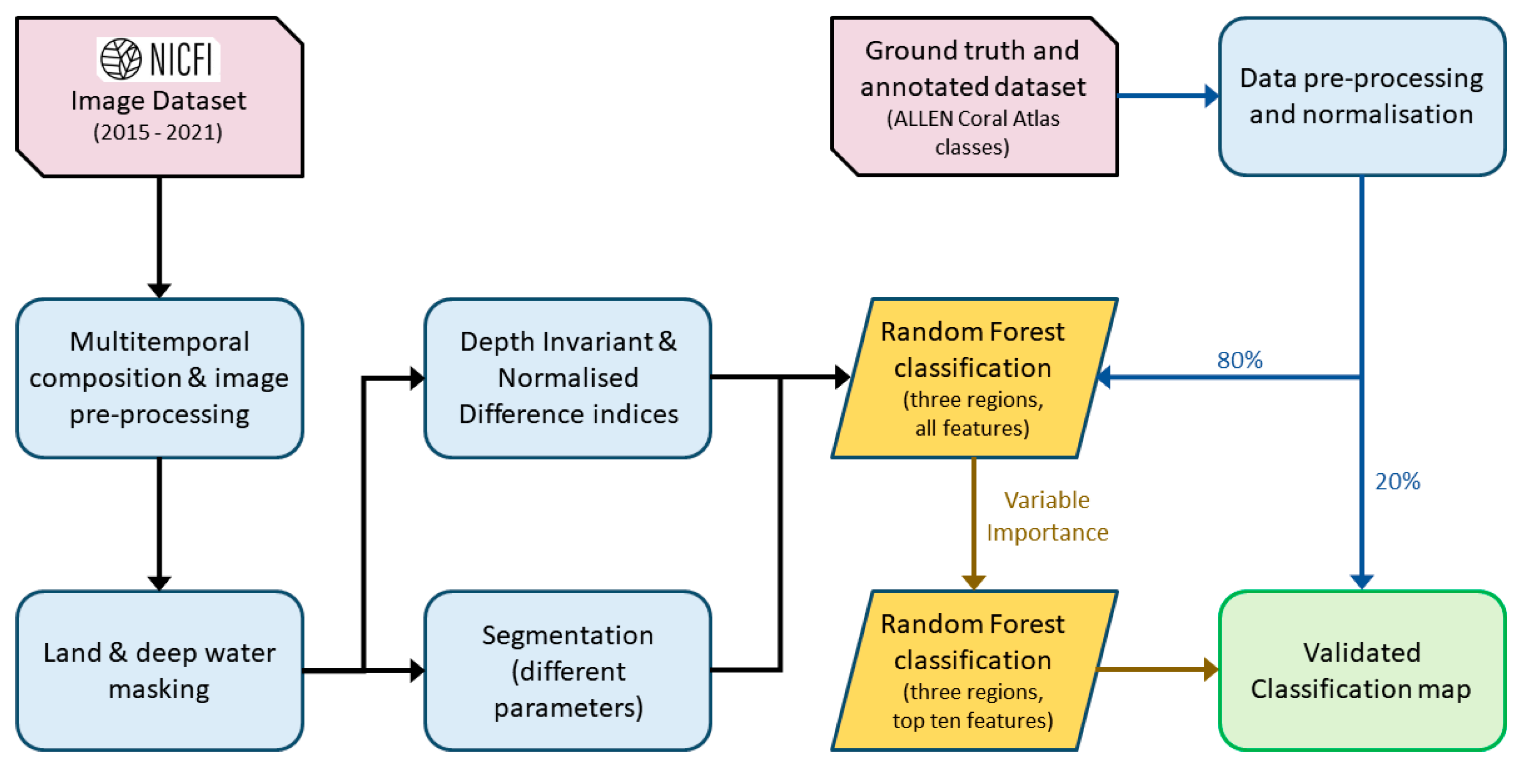
2.3. Earth Observation Framework

A fully cloud-native algorithmic framework was implemented for the data processing and image classification (Figure 3).

2.3.1. Multitemporal Data Analytics for Planet NICFI Basemaps

The NICFI half-yearly composite basemaps from 2015 to 2020 were selected, as the monthly composites from end-2020 onwards have issues with cloud and other atmospheric contamination. A multitemporal composition of 14 basemaps was then performed based on an interval mean of the 10th and 50th percentile. This statistical metric is the best-performing in this region over other approaches such as the 20th percentile, median, as well as other combinations of interval means. The lower and upper percentiles help to reduce the effects of the darker cloud shadows as well as the brighter sunglint and remnant clouds, respectively [53]. A mean of these two images combines their strengths together to produce a better composite. Furthermore, this approach alleviates the influence of tidal inundations [12].
The composite image was divided by pi to obtain the normalised water-leaving reflectance. Following, the land was masked using a Normalised Difference Water Index (NDWI) adapted from Landsat 8 [54] and proven useful in Sentinel-2 Surface Reflectance Products [53]. Deep water masking was performed using an adapted true colour HSV approach owing to the band limitations of PlanetScope [55], as well as manual masking for the pixels that were easily confused [41,49]. Owing to the limited number of spectral bands and the use of variable importance downstream to retain only the most useful features, the N band was retained for the downstream feature generation phase rather than removed by standard atmospheric correction. This prevents the overcorrection of aquatic pixels at the shallowest waters and allows the N band to be useful in detecting intertidal seagrasses [12,42].
To remain within the computational quota of GEE, the classification was separated into three geographical regions—north, central, and south (Figure 2). If the computational quota of GEE had been exceeded, then the code script would time out or terminate, depending on the type of error, and any uncompleted processes would fail to yield any valid results. For the same computational quota reason, the spatial resolution was computed at 5 m instead of 4.77 m.

2.3.2. Feature Engineering

Three methods were used in the feature generation phase: Normalised Difference indices, Depth Invariant Indices (DII), and segmentation.
All combinations of the four spectral bands were used to generate different Normalised Difference (ND) indices, including the Normalised Difference Vegetation Index (NDVI) and NDWI. Equation (1) shows the general equation for the Normalised Difference Index. As aforementioned, NDVI has been used for intertidal seagrass detection [12]. Although the NDWI might have been used upstream for land masking, it was bulk-produced and left to the variable importance approach downstream to weigh its contributions. Meanwhile, the blue and green bands are usually better for detection in deeper waters, as their penetration into the water column is better than red or near-infrared [51]. Thus, Normalised Difference Indices of blue and green combinations were also included in the analysis.
N o r m a l i s e d   D i f f e r e n c e i j = i j i + j   ,
where i and j are the bands used. Only a combination was used instead of the permutation, as the combination ij would be the negative of combination ji, meaning duplicated information.
The Depth Invariant Index was proposed by Lyzenga et al. [56], who found that two logarithmically-transformed bands showed a linear relationship with respect to relative depth, so long as the data are from the same class or cover. The DII is a good substitute for bathymetry and is thus used in a classification where bathymetric data are unavailable [56]. The same spectral band combinations as the ND indices were also used to derive different DII. The N band was included because there are linear relationships between the N band combinations similar to the concept of DII. While the blue (B) and green (G) bands are generally proposed for aquatic remote sensing [51], the band combination might also be situational and case-specific [57], thereby necessitating an analysis across the possible band combinations.
D e p t h   I n v a r i a n t   I n d e x i j = l n L i k i k j l n L j k i k j = a + a 2 + 1 a = σ i i σ j j 2 σ i j ,
where L i and L j are the reflectance values of bands i and j, k i k j is the ratio attenuation coefficient of bands i and j, σ i i is the variance of band i, σ j j is the variance of band j, and σ i j is the covariance of both bands i and j. The high spatial resolution of the NICFI basemaps allows for a finer object-based approach. The GEE-inbuilt Simple Non-Iterative Clustering (SNIC) segmentation function (ee.Algorithms.Image.Segmentation.SNIC) and the function to connect similar pixels based on the previous function into an object (ee.Image.reduceConnectedComponents) were used to produce the segmentation features [43]. The SNIC is a polygonal partitioning algorithm based on Simple Linear Iterative Clustering (SLIC), which segments an image into smaller polygons or superpixels using seeds or pixels selected from a grid [58]. Unlike SLIC, which involves multiple iterations of centroid computation per run, SNIC performs a constant calculation of centroid values after each pixel is assigned to a cluster, thereby allowing for the segmentation to be completed in one run without needing iterations [58]. As such, it is highly suitable for GEE, which is not iterative [19]. This approach was also used to enhance the classification and identification of different wetland types on GEE [59] and improve seagrass species identification in single PlanetScope images [44]. Parameter optimisation was performed for the segmentation seed grid size (seed grid) and compactness as well as for the maximum size of the reduced connected components (Reduce Connected Components) based on the overall accuracy of the classification. The tested ranges are 5, 10, and 15 for seed grid size, 0, 0.2, 0.4, 0.6, and 0.8 for compactness, and 10, 100, and 1000 for the reduced connected components. The grid size and reduced connected components cannot be increased further, given the size of the PlanetScope NICFI composite images in this study, or else the calculations would exceed the computational quota of GEE and not produce any valid results.

2.3.3. Normalisation of Reference Data

The processed image was then sampled with the cleaned reference data, which were then split into a training and test dataset in an 80:20 ratio. Following, the training dataset was normalised per class to remove the lowest 5-percentile and highest 10-percentile spectral values that might affect the classifier [21,52]. This would ensure that the trained classifier was not biased by any possible extreme or anomalous training data, which would allow it to be more suitable for transfer to other areas of the same geographic region. The test dataset was not normalised to maximise the amount of data points used for testing as well as to ensure that the quantitative penalty from misclassifications would not be reduced (Figure 4).

2.3.4. Classification

The Random Forest function in GEE (ee.Classifier.smileRandomForest) was used for classification using the default parameters [16,21,22,23], which includes a 50:50 random split of the training dataset for its training. The Random Forest model is a supervised machine-learning ensemble approach of many independent decision trees [60]. This model is robust against noise and overfitting [60] and is able to manage any collinearity or non-linearity between the predictor variables [61]. It has also performed well with high accuracies for coastal habitat mapping over a range of scales and in different parts of the world [21,22,23,50]. The model was first trained using only the training dataset with all the features before a variable importance (ee.Classifier.explain) was used to identify and extract the top ten features [21,42]. Then, the model was trained using the training dataset again with only these ten features for classification. The frequency plots of the features that are selected within the top ten features per region can be found in the Supplementary Materials.

2.4. Accuracy Assessment
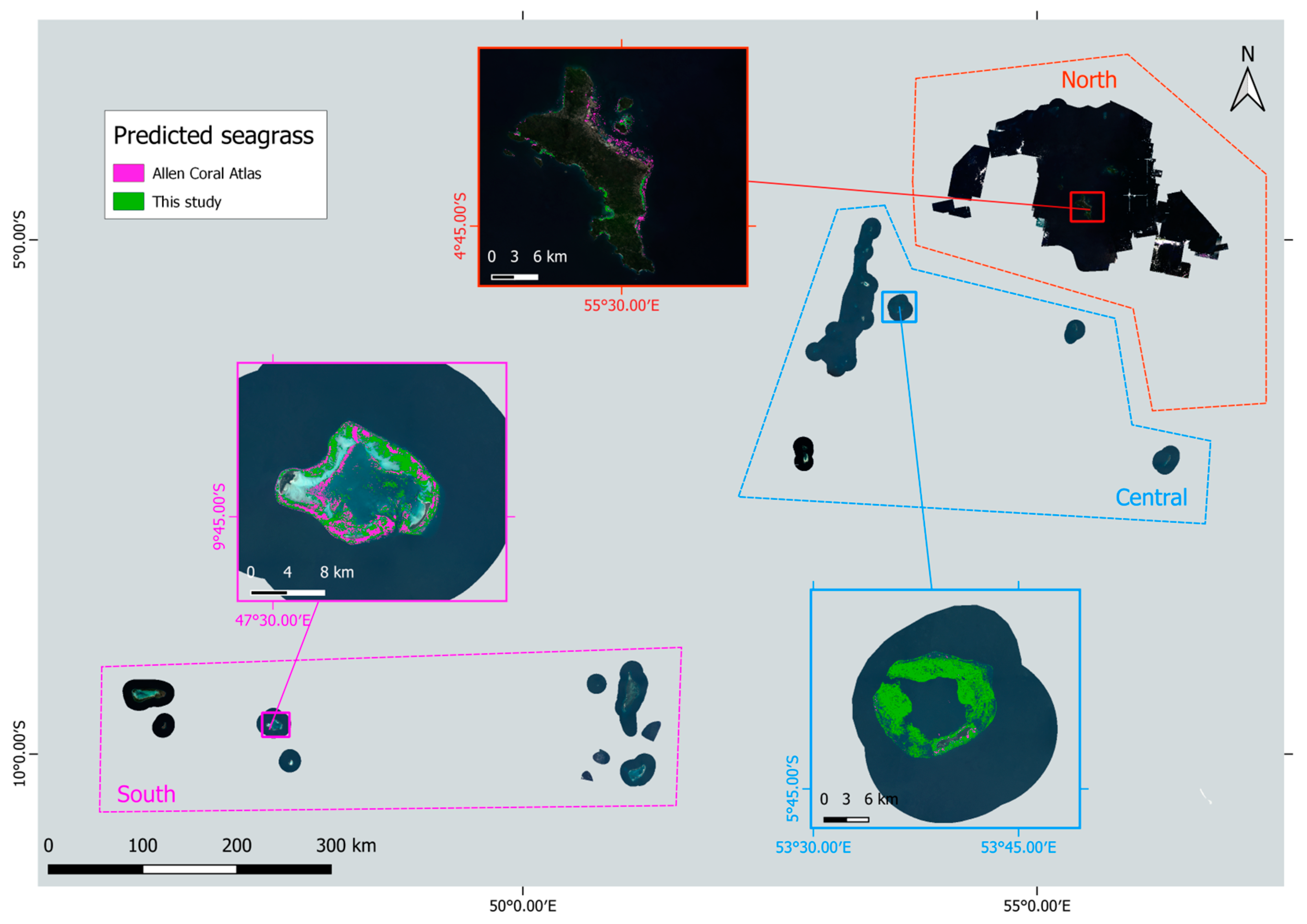
The performance of the classification was quantitatively assessed via the overall image accuracy, the seagrass-class producer’s and user’s accuracy, as well as the seagrass-class F1 score using the test dataset [16,21,22,23]. These metrics are commonly used in remote sensing [62]. Given a class i:
F 1 i = 2 × P A i × U A i P A i + U A i   C l a s s   P r o d u c e r s   A c c u r a c y ,   P A i = n u m b e r   o f   c o r r e c t l y   c l a s s i f i e d   s a m p l e s   f o r   c l a s s   i   n u m b e r   o f   s a m p l e s   i n   r e f e r e n c e   d a t a   f o r   c l a s s   i C l a s s   U s e r s   A c c u r a c y ,   U A i = n u m b e r   o f   c o r r e c t l y   c l a s s i f i e d   s a m p l e s   f o r   c l a s s   i   n u m b e r   o f   c l a s s i f i e d   s a m p l e s   f o r   c l a s s   i ,
The F1 score is bounded between 0 and 1, with higher values suggesting a better classification of class i. Nevertheless, a high F1 score may still be susceptible to commission errors, which happens with a high P A i and a low U A i , or omission errors, which is the converse. As such, the study would also consider the difference in P A i and U A i when understanding the possible errors in the resultant map.

3. Results

The classification with segmentation features achieved the best overall accuracies between 69.7% and 75.7%. The corresponding parameters for the segmentation functions are also reported in Table 2. The producer’s and user’s accuracy for the seagrass class in the north is similar at 62.6% and 63.9%, respectively, suggesting a good balance between sensitivity and specificity. In the two other regions, the producer’s accuracy of the seagrass class is greater than the user’s accuracy by at least 5%, which would suggest a tendency for commissioning errors and overestimation. Nonetheless, both regions had a better F1 score for the seagrass class than for the north.
A total of 798.97 km2 of seagrasses were identified, whose bulk is in the central and south regions. The north region had the least total predicted seagrass meadow at 39.41 km2, while the central region had the most at 428.18 km2 (Table 3). Most of the predicted seagrass areas in the north are located around the Inner Islands of Mahé, Praslin, and La Digue, as well as at Denis and Bird Islands.
Compared to the Allen Coral Atlas (ACA) project, which does not map deeper seagrasses (below 10 m) [50], more seagrasses were mapped in the deeper central region in this study (Figure 4). More shallow seagrasses were predicted in the north and south regions by this study as compared to the ACA. However, the deeper seagrasses could not be mapped in the north, as there was confusion between the darker seagrass cover and the dark optically deep waters owing to insufficient training data for seagrasses in those deeper extents. There was also some misclassification by ACA at Cosmoledo in the south (Figure 5), which was suppressed by the deep water mask in this study.

4. Discussion

This study is the first to explore the suitability of the high spatial resolution NICFI basemaps to map and estimate the national seagrass extent and optically shallow seabed of a given country; in our case study, this of archipelagic Seychelles. A total of 798.97 km2 of seagrass meadows was mapped to an accuracy between 69.7% and 75.7%. Such application is beyond the intended use of these NICFI basemaps [26,43] and thereby expands the applications of these basemaps. Furthermore, with the restricted options for benthic remote sensing, the possibility of an alternative product or data source is helpful and broadens the available options for the task. In this study, the insufficient coverage by Sentinel-2 over the Seychelles would have meant that much of the central region of the Seychelles could possibly not have been mapped (Figure 2). Beyond seagrasses, the NICFI basemaps could also be used for other coastal, intertidal, and nearshore marine habitats, such as coral reefs and algae. The increased spatial resolution of NICFI provides the potential for a finer-scaled map than Sentinel-2 (Table 1). The use of reference data collected from accessible regions allowed map-based estimates of seagrasses in less accessible islands, atolls, and offshore banks. Without the judicious use of reference data, these less accessible places are unable to be mapped, and their seagrass meadows could not be fully accounted for within the NDCs.
The mapped seagrasses in this study are substantially less than the seagrass extent of 20,831.68 km2 reported in an earlier ecosystem services report [31], based on photointerpretation of satellite imagery. In comparison, the use of a reproducible classification model reduces the subjectivity that might be incurred during photointerpretation. By leveraging the power of cloud computing and parallel processing [21,22,23], an area as large as Seychelles can be quickly mapped over the required time and labour needed for the photointerpretation approach. Meanwhile, version 7 of the UNEP-WCMC seagrass dataset of the Seychellois seagrass contained only point and no polygon data in the region; hence, no meaningful comparisons could be made [63]. The Allen Coral Atlas Benthic Layer of Seychelles mapped seagrasses only up to 10 m in depth, provided a national estimate of 207.03 km2, and excluded the deeper reef seagrasses found in the central region. Furthermore, the training dataset used in the present study is obtained by local experts and collaborators. As such, these mapped areas provide a better estimate of the actual seagrass distribution in the Seychelles currently and contribute to filling knowledge gaps in the global seagrass extent [6]. Addressing these gaps will better inform scientific research and management policies that rely on such data in turn.

4.1. Challenges

Despite its potential, the NICFI basemaps face challenges with their four-band spectral resolution. Furthermore, the lack of reference data designed for remote sensing research would introduce more uncertainties in the results [49]. In conjunction, it would naturally stress the image processing, which again leads to more uncertainties.
Owing to the physics of light travelling through a water column [64], the suitable range of optical wavelengths is generally restricted to the visible spectrum [51]. Seagrass may have similar spectral profiles as certain greener macroalgae species or appear brown in different conditions that confuse it instead with brown macroalgae [41,42,65]. This was partly mitigated with the addition of features [43,44,56]. Although the derived features would have some correlation with its source band(s), the improved quantitative and qualitative results demonstrate their use to alleviate the low spectral feature space of the NICFI basemaps while not substantially under or overestimating the seagrass meadows. Similarly, Vizzari et al. [43] achieved better results with an object-based Random Forest classification on NICFI basemaps over the Sentinel-2 images for terrestrial forest detection, thereby further enforcing the use of feature generation to improve the classification.
Uncertainties may also arise from the reference dataset. An ideal dataset for remote sensing should be balanced and representative of the whole image [52]. Unfortunately, the inaccessibility to the banks around the northern plateau and many Outer Islands compared to the inhabited areas of the Inner Islands would naturally bias the collected data to the areas of easy access [29]. It is costly to organise field surveys in less accessible places, and even citizen science is susceptible to spatio-temporal clustering bias related to accessibility or popularity [66]. To illustrate, the low availability of deeper seagrass spatial data came from a reuse of data designed for other purposes, such as coring at deeper depths [49]. Processing the reference data to fit remote sensing research introduces its own uncertainties, even as it alleviates other issues, such as anomalous values or comparability between different classes [21].
While PlanetScope had normalised and harmonised their NICFI basemaps using Landsat data with the purpose of detecting deforestation, these basemaps are not a product of a radiative transfer model [26]. This aligns with a recommendation to correct the images with a data fusion approach made by Frazier and Hemingway on some of the shortcomings of PlanetScope images [67]. Additionally, the multitemporal composite of the composites leverages a statistical approach to further reduce possible anomalies [54]. Although a region of the Seychelles was not captured by Sentinel-2 until mid-2021, this is unlikely for other sites globally. As such, future alternatives include data harmonisation and/or fusion with Sentinel-2 to improve its image quality while retaining its high spatial resolution [68].
Ultimately, the NICFI basemaps are terrestrially focused [26]; thus, there is a limit to its coastal buffer. For offshore shallow reefs that are substantial and still visible via satellite imagery, some of these reefs and seagrass meadows lie outside of the NICFI basemaps. As such, supplementary datasets, such as Sentinel-2, had to be included to fully comprise the national extent of the Seychellois seagrass meadows [28].

4.2. Transferability

So long as the shortfalls of the NICFI basemaps are both considered and managed, NICFI is easily incorporated into GEE workflows to create seagrass maps of better spatial resolution than other publicly available satellite imagery such as Sentinel-2 and Landsat 8. The ability to transfer methods across multiple data sources is also well demonstrated by this study, as much of the framework was originally developed on Sentinel-2 imagery [16,22]. Owing to spectral and spatial resolution differences as well as the nature of the NICFI basemaps as image composites (Table 1), some adaptations and finetuning of processing workflows are to be expected. The workflow identified here can, however, be easily transferred to other sites. It is highly accessible to aspiring researchers or managers and has a relatively low barrier of knowledge to entry [16]. The resulting spatially explicit maps and estimates are expected to aid blue carbon accounting efforts, such as for the Seychelles’ Blue Economy [40], in order to achieve a tangible outcome for the conservation and management of seagrasses based on data-driven Earth Observation science.

4.3. Beyond PlanetScope

This study showcases the potential for broader use of NICFI basemaps for seagrass and other benthic seafloor mapping at scale. The scope of this study is strictly the analysis of NICFI basemaps for mapping seagrasses. As such, it is not recommended to quote the area estimates by the NICFI basemap in this study (Table 3) and to instead refer to Rowlands et al. [28] for the best seagrass estimates based on the combined results of this study, Sentinel-2, and other datasets. Nevertheless, this successful use of NICFI basemaps suggests that it might be premature to discount NICFI basemaps or any other imagery for the use of aquatic applications, especially if more broadly applied options are not feasible or available for a specific application or area.

5. Conclusions

The NICFI basemap composite based on an interval mean of 10 and 50 percentiles was able to classify seagrasses in Seychelles to a high level of accuracy. Not only does it showcase that the NICFI basemaps could be applied beyond the original scope of terrestrial applications (forest and NDVI monitoring) originally envisaged, but the ability to map out some of the deeper seagrass meadows compared to its contemporaries suggests a multisensory approach may be required to deliver seagrass mapping and monitoring objectives at national to global scales. While challenges remain, this blueprint project and mapping endeavour demonstrate the potential of the NICFI basemaps on GEE to contribute to seagrass mapping, climate change agendas, national blue carbon accounting, and the conservation of seagrasses across national scales.

Supplementary Materials

The following supporting information can be downloaded at https://www.mdpi.com/article/10.3390/rs15184500/s1.

Author Contributions

Conceptualization, D.T. and G.R.; methodology, C.B.L., D.T., L.M. and G.R.; software, C.B.L.; validation, C.B.L., L.M. and G.R.; formal analysis, C.B.L., D.T., L.M. and G.R.; investigation, C.B.L.; resources, S.A., S.K.B., A.C., A.F., J.H., M.M., J.A.M., L.M. and G.R.; data curation, C.B.L., D.T., L.M. and G.R.; writing—original draft preparation, C.B.L.; writing—review and editing, C.B.L., D.T., L.M., S.A., S.K.B., A.C., A.F., J.H., M.M., J.A.M. and G.R.; visualisation, C.B.L.; supervision, P.R. and G.R.; project administration, D.T. and G.R.; funding acquisition, G.R. All authors have read and agreed to the published version of the manuscript.

Funding

Support for this project was provided by The Pew Charitable Trusts (No. 34376). The views expressed herein are those of the author(s) and do not necessarily reflect the views of The Pew Charitable Trusts. C.B.L. is supported by the DLR-DAAD Research Fellowship (No. 57478193). D.T. is funded by DLR through the Global Seagrass Watch technology marketing project.

Data Availability Statement

Mapping data are available upon request due to restrictions. The satellite data presented in this study are available upon request from the corresponding author. The reference data are not publicly available due to licences with the Seychelles government.

Acknowledgments

We thank Spyridon Christofilakos (DLR) for his feedback on the draft manuscript. This data have been provided under the NICFI Satellite Data Program.

Conflicts of Interest

The authors declare no conflict of interest. The funders had no role in the design of the study, in the collection, analyses, or interpretation of data, in the writing of the manuscript, or in the decision to publish the results.

References

  1. Davidson, N.C.; van Dam, A.A.; Finlayson, C.M.; McInnes, R.J. Worth of wetlands: Revised global monetary values of coastal and inland wetland ecosystem services. Mar. Freshw. Res. 2019, 70, 1189–1194. [Google Scholar] [CrossRef]
  2. Malerba, M.E.; Duarte de Paula Costa, M.; Friess, D.A.; Schuster, L.; Young, M.A.; Lagomasino, D.; Serrano, O.; Hickey, S.M.; York, P.H.; Rasheed, M.; et al. Remote sensing for cost-effective blue carbon accounting. Earth-Sci. Rev. 2023, 238, 104337. [Google Scholar] [CrossRef]
  3. Unsworth, R.K.F.; Nordlund, L.M.; Cullen-Unsworth, L.C. Seagrass meadows support global fisheries production. Conserv. Lett. 2019, 12, e12566. [Google Scholar] [CrossRef]
  4. Hughes, A.R.; Williams, S.L.; Duarte, C.M.; Heck, K.L., Jr.; Waycott, M. Associations of concern: Declining seagrasses and threatened dependent species. Front. Ecol. Environ. 2009, 7, 242–246. [Google Scholar] [CrossRef]
  5. de los Santos, C.B.; Olivé, I.; Moreira, M.; Silva, A.; Freitas, C.; Araújo Luna, R.; Quental-Ferreira, H.; Martins, M.; Costa, M.M.; Silva, J.; et al. Seagrass meadows improve inflowing water quality in aquaculture ponds. Aquaculture 2020, 528, 735502. [Google Scholar] [CrossRef]
  6. Dunic, J.C.; Brown, C.J.; Connolly, R.M.; Turschwell, M.P.; Côté, I.M. Long-term declines and recovery of meadow area across the world’s seagrass bioregions. Glob. Change Biol. 2021, 27, 4096–4109. [Google Scholar] [CrossRef]
  7. Duffy, J.E.; Benedetti-Cecchi, L.; Trinanes, J.; Muller-Karger, F.E.; Ambo-Rappe, R.; Boström, C.; Buschmann, A.H.; Byrnes, J.; Coles, R.G.; Creed, J.; et al. Toward a Coordinated Global Observing System for Seagrasses and Marine Macroalgae. Front. Mar. Sci. 2019, 6, 317. [Google Scholar] [CrossRef]
  8. Waycott, M.; Duarte, C.M.; Carruthers, T.J.B.; Orth, R.J.; Dennison, W.C.; Olyarnik, S.; Calladine, A.; Fourqurean, J.W.; Heck, K.L.; Hughes, A.R.; et al. Accelerating loss of seagrasses across the globe threatens coastal ecosystems. Proc. Natl. Acad. Sci. USA 2009, 106, 12377–12381. [Google Scholar] [CrossRef]
  9. Fortes, M.D.; Ooi, J.L.S.; Tan, Y.M.; Prathep, A.; Bujang, J.S.; Yaakub, S.M. Seagrass in Southeast Asia: A review of status and knowledge gaps, and a road map for conservation. Bot. Mar. 2018, 61, 269–288. [Google Scholar] [CrossRef]
  10. Mtwana Nordlund, L.; Koch, E.W.; Barbier, E.B.; Creed, J.C. Seagrass Ecosystem Services and Their Variability across Genera and Geographical Regions. PLoS ONE 2016, 11, e0163091. [Google Scholar] [CrossRef]
  11. Losciale, R.; Day, J.; Heron, S. Conservation status, research, and knowledge of seagrass habitats in World Heritage properties. Conserv. Sci. Pract. 2022, 4, e12830. [Google Scholar] [CrossRef]
  12. Zhou, Q.; Ke, Y.; Wang, X.; Bai, J.; Zhou, D.; Li, X. Developing seagrass index for long term monitoring of Zostera japonica seagrass bed: A case study in Yellow River Delta, China. ISPRS J. Photogramm. Remote Sens. 2022, 194, 286–301. [Google Scholar] [CrossRef]
  13. Unsworth, R.K.F.; McKenzie, L.J.; Collier, C.J.; Cullen-Unsworth, L.C.; Duarte, C.M.; Eklöf, J.S.; Jarvis, J.C.; Jones, B.L.; Nordlund, L.M. Global challenges for seagrass conservation. Ambio 2019, 48, 801–815. [Google Scholar] [CrossRef]
  14. Losciale, R.; Hay, R.; Rasheed, M.; Heron, S. ‘The public perception of the role, importance, and vulnerability of seagrass. A case study from the Great Barrier Reef’. Environ. Dev. 2022, 44, 100757. [Google Scholar] [CrossRef]
  15. Buelow, C.A.; Connolly, R.M.; Turschwell, M.P.; Adame, M.F.; Ahmadia, G.N.; Andradi-Brown, D.A.; Bunting, P.; Canty, S.W.J.; Dunic, J.C.; Friess, D.A.; et al. Ambitious global targets for mangrove and seagrass recovery. Curr. Biol. 2022, 32, 1641–1649.e1643. [Google Scholar] [CrossRef]
  16. Traganos, D.; Aggarwal, B.; Poursanidis, D.; Topouzelis, K.; Chrysoulakis, N.; Reinartz, P. Towards Global-Scale Seagrass Mapping and Monitoring Using Sentinel-2 on Google Earth Engine: The Case Study of the Aegean and Ionian Seas. Remote Sens. 2018, 10, 1227. [Google Scholar] [CrossRef]
  17. Phinn, S.; Roelfsema, C.; Kovacs, E.; Canto, R.; Lyons, M.; Saunders, M.; Maxwell, P. Mapping, Monitoring and Modelling Seagrass Using Remote Sensing Techniques. In Seagrasses of Australia: Structure, Ecology and Conservation; Larkum, A.W.D., Kendrick, G.A., Ralph, P.J., Eds.; Springer International Publishing: Cham, Switzerland, 2018; pp. 445–487. [Google Scholar]
  18. Rowlands, G.; Purkis, S.; Riegl, B.; Metsamaa, L.; Bruckner, A.; Renaud, P. Satellite imaging coral reef resilience at regional scale. A case-study from Saudi Arabia. Mar. Pollut. Bull. 2012, 64, 1222–1237. [Google Scholar] [CrossRef] [PubMed]
  19. Gorelick, N.; Hancher, M.; Dixon, M.; Ilyushchenko, S.; Thau, D.; Moore, R. Google Earth Engine: Planetary-scale geospatial analysis for everyone. Remote Sens. Environ. 2017, 202, 18–27. [Google Scholar] [CrossRef]
  20. Yang, H.; Kong, J.; Hu, H.; Du, Y.; Gao, M.; Chen, F. A Review of Remote Sensing for Water Quality Retrieval: Progress and Challenges. Remote Sens. 2022, 14, 1770. [Google Scholar] [CrossRef]
  21. Blume, A.; Pertiwi, A.P.; Lee, C.B.; Traganos, D. Bahamian seagrass extent and blue carbon accounting using Earth Observation. Front. Mar. Sci. 2023, 10, 1058460. [Google Scholar] [CrossRef]
  22. Traganos, D.; Lee, C.B.; Blume, A.; Poursanidis, D.; Čižmek, H.; Deter, J.; Mačić, V.; Montefalcone, M.; Pergent, G.; Pergent-Martini, C.; et al. Spatially Explicit Seagrass Extent Mapping Across the Entire Mediterranean. Front. Mar. Sci. 2022, 9, 871799. [Google Scholar] [CrossRef]
  23. Traganos, D.; Pertiwi, A.P.; Lee, C.B.; Blume, A.; Poursanidis, D.; Shapiro, A. Earth observation for ecosystem accounting: Spatially explicit national seagrass extent and carbon stock in Kenya, Tanzania, Mozambique and Madagascar. Remote Sens. Ecol. Conserv. 2022, 8, 778–792. [Google Scholar] [CrossRef]
  24. Trinh, X.T.; Takeuchi, W. 30 Years National Scale Seagrass Mapping in Vietnam with Landsat and Sentinel Imagery on Google Earth Engine. In Proceedings of the 40th Asian Conference on Remote Sensing (ACRS 2019), Daejeon, Republic of Korea, 14–18 October 2019. [Google Scholar]
  25. Sebastian, T.; Sreenath, K.R.; Sreeram, M.P.; Ranith, R. Dwindling seagrasses: A multi-temporal analysis on Google Earth Engine. Ecol. Inform. 2023, 74, 101964. [Google Scholar] [CrossRef]
  26. Planet Team. Planet Application Program Interface: In Space for Life on Earth. 2017. Available online: https://api.planet.com (accessed on 1 December 2022).
  27. Sano, E.E.; Bolfe, É.L.; Parreiras, T.C.; Bettiol, G.M.; Vicente, L.E.; Sanches, I.D.A.; Victoria, D.d.C. Estimating Double Cropping Plantations in the Brazilian Cerrado through PlanetScope Monthly Mosaics. Land 2023, 12, 581. [Google Scholar] [CrossRef]
  28. Rowlands, G.; Antat, S.; Baez, S.; Cupidon, A.; Faure, A.; Harlay, J.; Lee, C.; Martin, L.; Masque, P.; Morgan, M.; et al. The Seychelles Seagrass Mapping and Carbon Assessment; Government of Seychelles, Ministry of Agriculture: Victoria Mahe, Seychelles, 2023.
  29. Central Intelligence Agency. The World Factbook 2021: Seychelles. Available online: https://www.cia.gov/the-world-factbook/countries/seychelles/ (accessed on 15 March 2023).
  30. Benzaken, D.; Hoareau, K. From concept to practice: The blue economy in Seychelles. In The Blue Economy in Sub-Saharan Africa: Working for a Sustainable Future; Sparks, D., Ed.; Routledge: London, UK, 2021; pp. 143–157. [Google Scholar]
  31. The Nature Conservancy. Evaluation of Ecosystem Goods and Services for Seychelles’ Existing and Proposed Protected Area System; An Unpublished Report to Government of Seychelles—MACCE and SWIOFish3 Programme; The Nature Conservancy: Arlington, VA, USA, 2022; p. 78. [Google Scholar]
  32. Chanda, A. Blue Carbon Dynamics in the Indian Ocean Seagrass Ecosystems. In Blue Carbon Dynamics of the Indian Ocean, 1st ed.; Chanda, A., Das, S., Ghosh, T., Eds.; Springer: Cham, Switzerland, 2022; pp. 145–169. [Google Scholar]
  33. Hamylton, S.; Hagan, A.; Bunbury, N.; Fleischer-Dogley, F.; Spencer, T. Mapping the Lagoon at Aldabra Atoll, Western Indian Ocean; Papers: Part B; University of Wollongong, Faculty of Science, Medicine and Health: Wollongong, NSW, Australia, 2018. [Google Scholar]
  34. Payet, R.; Agricole, W. Climate Change in the Seychelles: Implications for Water and Coral Reefs. AMBIO A J. Hum. Environ. 2006, 35, 182–189. [Google Scholar] [CrossRef]
  35. Duarte, B.; Martins, I.; Rosa, R.; Matos, A.R.; Roleda, M.Y.; Reusch, T.B.H.; Engelen, A.H.; Serrão, E.A.; Pearson, G.A.; Marques, J.C.; et al. Climate Change Impacts on Seagrass Meadows and Macroalgal Forests: An Integrative Perspective on Acclimation and Adaptation Potential. Front. Mar. Sci. 2018, 5, 190. [Google Scholar] [CrossRef]
  36. Ingram, J.C.; Dawson, T.P. The impacts of a river effluent on the coastal seagrass habitats of Mahé, Seychelles. S. Afr. J. Bot. 2001, 67, 483–487. [Google Scholar] [CrossRef]
  37. Mackie, A.S.Y.; Oliver, P.G.; Darbyshire, T.; Mortimer, K. Shallow marine benthic invertebrates of the Seychelles Plateau: High diversity in a tropical oligotrophic environment. Philos. Trans. R. Soc. A Math. Phys. Eng. Sci. 2005, 363, 203–228. [Google Scholar] [CrossRef]
  38. Barnes, D.K.A.; Barnes, R.S.K.; Smith, D.J.; Rothery, P.; Coral & Coastal Ecology of the Seychelles Research Programme. Littoral biodiversity across scales in the Seychelles, Indian Ocean. Mar. Biodivers. 2009, 39, 109–119. [Google Scholar] [CrossRef]
  39. Daly, R.; Stevens, G.; Daly, C.K. Rapid marine biodiversity assessment records 16 new marine fish species for Seychelles, West Indian Ocean. Mar. Biodivers. Rec. 2018, 11, 6. [Google Scholar] [CrossRef]
  40. Schutter, M.S.; Hicks, C.C. Networking the Blue Economy in Seychelles: Pioneers, resistance, and the power of influence. J. Political Ecol. 2019, 26, 425–447. [Google Scholar] [CrossRef]
  41. Lizcano-Sandoval, L.; Anastasiou, C.; Montes, E.; Raulerson, G.; Sherwood, E.; Muller-Karger, F.E. Seagrass distribution, areal cover, and changes (1990–2021) in coastal waters off West-Central Florida, USA. Estuar. Coast. Shelf Sci. 2022, 279, 108134. [Google Scholar] [CrossRef]
  42. Wicaksono, P.; Maishella, A.; Wahyudi, A.a.J.; Hafizt, M. Multitemporal seagrass carbon assimilation and aboveground carbon stock mapping using Sentinel-2 in Labuan Bajo 2019–2020. Remote Sens. Appl. Soc. Environ. 2022, 27, 100803. [Google Scholar] [CrossRef]
  43. Vizzari, M. PlanetScope, Sentinel-2, and Sentinel-1 Data Integration for Object-Based Land Cover Classification in Google Earth Engine. Remote Sens. 2022, 14, 2628. [Google Scholar] [CrossRef]
  44. Wicaksono, P.; Lazuardi, W. Assessment of PlanetScope images for benthic habitat and seagrass species mapping in a complex optically shallow water environment. Int. J. Remote Sens. 2018, 39, 5739–5765. [Google Scholar] [CrossRef]
  45. Roca, M.; Navarro, G.; García-Sanabria, J.; Caballero, I. Monitoring Sand Spit Variability Using Sentinel-2 and Google Earth Engine in a Mediterranean Estuary. Remote Sens. 2022, 14, 2345. [Google Scholar] [CrossRef]
  46. Roy, D.P.; Huang, H.; Boschetti, L.; Giglio, L.; Yan, L.; Zhang, H.H.; Li, Z. Landsat-8 and Sentinel-2 burned area mapping—A combined sensor multi-temporal change detection approach. Remote Sens. Environ. 2019, 231, 111254. [Google Scholar] [CrossRef]
  47. Thales Alenia Space. Sentinel-2 Products Specification Document. Sentinel 2 Document Library. 2022, p. 552. Available online: https://sentinel.esa.int/web/sentinel/user-guides/sentinel-2-msi/document-library/-/asset_publisher/Wk0TKajiISaR/content/sentinel-2-level-1-to-level-1c-product-specifications (accessed on 1 December 2022).
  48. Roy, D.P.; Huang, H.; Houborg, R.; Martins, V.S. A global analysis of the temporal availability of PlanetScope high spatial resolution multi-spectral imagery. Remote Sens. Environ. 2021, 264, 112586. [Google Scholar] [CrossRef]
  49. Kovacs, E.M.; Roelfsema, C.; Udy, J.; Baltais, S.; Lyons, M.; Phinn, S. Cloud Processing for Simultaneous Mapping of Seagrass Meadows in Optically Complex and Varied Water. Remote Sens. 2022, 14, 609. [Google Scholar] [CrossRef]
  50. Lyons, M.B.; Roelfsema, C.M.; Kennedy, E.V.; Kovacs, E.M.; Borrego-Acevedo, R.; Markey, K.; Roe, M.; Yuwono, D.M.; Harris, D.L.; Phinn, S.R.; et al. Mapping the world’s coral reefs using a global multiscale earth observation framework. Remote Sens. Ecol. Conserv. 2020, 6, 557–568. [Google Scholar] [CrossRef]
  51. Li, J.; Fabina, N.S.; Knapp, D.E.; Asner, G.P. The Sensitivity of Multi-spectral Satellite Sensors to Benthic Habitat Change. Remote Sens. 2020, 12, 532. [Google Scholar] [CrossRef]
  52. Millard, K.; Richardson, M. On the Importance of Training Data Sample Selection in Random Forest Image Classification: A Case Study in Peatland Ecosystem Mapping. Remote Sens. 2015, 7, 8489–8515. [Google Scholar] [CrossRef]
  53. Cordeiro, M.C.R.; Martinez, J.-M.; Peña-Luque, S. Automatic water detection from multidimensional hierarchical clustering for Sentinel-2 images and a comparison with Level 2A processors. Remote Sens. Environ. 2021, 253, 112209. [Google Scholar] [CrossRef]
  54. Donchyts, G.; Schellekens, J.; Winsemius, H.; Eisemann, E.; Van de Giesen, N. A 30 m Resolution Surface Water Mask Including Estimation of Positional and Thematic Differences Using Landsat 8, SRTM and OpenStreetMap: A Case Study in the Murray-Darling Basin, Australia. Remote Sens. 2016, 8, 386. [Google Scholar] [CrossRef]
  55. Lee, C.B.; Traganos, D.; Reinartz, P. A Simple Cloud-Native Spectral Transformation Method to Disentangle Optically Shallow and Deep Waters in Sentinel-2 Images. Remote Sens. 2022, 14, 590. [Google Scholar] [CrossRef]
  56. Lyzenga, D.R.; Malinas, N.P.; Tanis, F.J. Multispectral bathymetry using a simple physically based algorithm. IEEE Trans. Geosci. Remote Sens. 2006, 44, 2251–2259. [Google Scholar] [CrossRef]
  57. Hamylton, S. An evaluation of waveband pairs for water column correction using band ratio methods for seabed mapping in the Seychelles. Int. J. Remote Sens. 2011, 32, 9185–9195. [Google Scholar] [CrossRef]
  58. Achanta, R.; Süsstrunk, S. Superpixels and Polygons Using Simple Non-iterative Clustering. In Proceedings of the 2017 IEEE Conference on Computer Vision and Pattern Recognition (CVPR), Honolulu, HI, USA, 21–26 July 2017; pp. 4895–4904. [Google Scholar]
  59. Liu, Z.Y.-C.; Chamberlin, A.J.; Tallam, K.; Jones, I.J.; Lamore, L.L.; Bauer, J.; Bresciani, M.; Wolfe, C.M.; Casagrandi, R.; Mari, L.; et al. Deep Learning Segmentation of Satellite Imagery Identifies Aquatic Vegetation Associated with Snail Intermediate Hosts of Schistosomiasis in Senegal, Africa. Remote Sens. 2022, 14, 1345. [Google Scholar] [CrossRef]
  60. Breiman, L. Random Forests. Mach. Learn. 2001, 45, 5–32. [Google Scholar] [CrossRef]
  61. Gislason, P.O.; Benediktsson, J.A.; Sveinsson, J.R. Random Forests for land cover classification. Pattern Recognit. Lett. 2006, 27, 294–300. [Google Scholar] [CrossRef]
  62. Maxwell, A.E.; Warner, T.A. Thematic Classification Accuracy Assessment with Inherently Uncertain Boundaries: An Argument for Center-Weighted Accuracy Assessment Metrics. Remote Sens. 2020, 12, 1905. [Google Scholar] [CrossRef]
  63. NEP-WCMC, Short FT. Global Distribution of Seagrasses (Version 7.1). Seventh Update to the Data Layer Used in Green and Short (2003). 2021. Available online: https://data.unep-wcmc.org/datasets/7 (accessed on 1 February 2023).
  64. Lee, Z.; Carder, K.L.; Mobley, C.D.; Steward, R.G.; Patch, J.S. Hyperspectral remote sensing for shallow waters. I. A semianalytical model. Appl. Opt. 1998, 37, 6329–6338. [Google Scholar] [CrossRef] [PubMed]
  65. Bannari, A.; Ali, T.S.; Abahussain, A. The capabilities of Sentinel-MSI (2A/2B) and Landsat-OLI (8/9) in seagrass and algae species differentiation using spectral reflectance. Ocean Sci. 2022, 18, 361–388. [Google Scholar] [CrossRef]
  66. Bird, T.J.; Bates, A.E.; Lefcheck, J.S.; Hill, N.A.; Thomson, R.J.; Edgar, G.J.; Stuart-Smith, R.D.; Wotherspoon, S.; Krkosek, M.; Stuart-Smith, J.F.; et al. Statistical solutions for error and bias in global citizen science datasets. Biol. Conserv. 2014, 173, 144–154. [Google Scholar] [CrossRef]
  67. Frazier, A.E.; Hemingway, B.L. A Technical Review of Planet Smallsat Data: Practical Considerations for Processing and Using PlanetScope Imagery. Remote Sens. 2021, 13, 3930. [Google Scholar] [CrossRef]
  68. Kwan, C.; Zhu, X.; Gao, F.; Chou, B.; Perez, D.; Li, J.; Shen, Y.; Koperski, K.; Marchisio, G. Assessment of Spatiotemporal Fusion Algorithms for Planet and Worldview Images. Sensors 2018, 18, 1051. [Google Scholar] [CrossRef]
Figure 1. Map of the Seychellois NICFI composite image with the mapped seagrass extent in green derived from this study, Sentinel-2, as well as the previous dataset [28]. The three geographical regions adopted by this study are also displayed here. The north region had the most reef seagrasses that were not captured by the NICFI image.
Remotesensing 15 04500 g001
Figure 2. The dates of the earliest Sentinel-2 images, based on Military Grid Reference System tiles, for Seychelles.
Remotesensing 15 04500 g002
Figure 3. Schematic workflow.
Remotesensing 15 04500 g003
Figure 4. Boxplot showing the class spectral profiles of the normalised training (left) and original validation (right) dataset for each class in the north region for (a) the original spectral bands, (b) the Normalised Difference indices, and (c) the Depth Invariant Indices.
Remotesensing 15 04500 g004aRemotesensing 15 04500 g004b
Figure 5. The predicted seagrass areas of the Allen Coral Atlas (purple) and our study (green) in Seychelles. One island from each region is displayed in the greater zoom, namely Mahé, Desroches, and Cosmoledo.
Remotesensing 15 04500 g005
Table 1. Attributes of Sentinel-2 imagery [47] against PlanetScope NICFI basemaps [26].
PlanetScope NICFISentinel-2
Temporal RangeDecember 2015 to presentJune 2015 to present (Level 1)
March 2017 to present (Level 2)
Image TypeHalf-yearly composite (December 2015 to August 2020)
Monthly composite (September 2020 to present)
Single Images
Image LevelSurface reflectanceTop of Atmosphere (Level 1)
Surface Reflectance (Level 2)
Spectral ResolutionFour bands (R, G, B, N)13 bands
Spatial Resolution4.77 m10 m
20 m
60 m
Temporal Resolution of Sensor36 h on average [48]5 days
Pre-processing/Atmospheric CorrectionMODIS-based atmospheric correction
Normalisation and harmonisation to Landsat SR data
Radiometric correction, Orthorectification (Level 1)
Atmospheric correction (Level 2)
Table 2. Classification accuracies of the best segmentation parameters. The optimised parameters are also given in this table.
NorthCentralSouth
Overall Accuracy69.7%73.4%75.7%
Producer’s Accuracy (seagrass)62.6%89.2%86.9%
User’s Accuracy (seagrass)63.9%77.7%81.5%
F1 score (seagrass)63.3%83.1%84.1%
Seed Grid size101515
Compactness0.60.60.8
Size for Reduce Connected Components10001001000
Table 3. Estimated seagrass extent in Seychelles by region based on this study, the Allen Coral Atlas, and a combined approach using this study, Sentinel-2, expert knowledge, and other datasets [28].
RegionTotal Predicted Seagrass Area (km2)
Planet NICFIAllen Coral AtlasCombined Approach
North39.417.48356.90
Central428.1824.72725.82
South331.38174.63337.93
Total798.97206.831420.65
Disclaimer/Publisher’s Note: The statements, opinions and data contained in all publications are solely those of the individual author(s) and contributor(s) and not of MDPI and/or the editor(s). MDPI and/or the editor(s) disclaim responsibility for any injury to people or property resulting from any ideas, methods, instructions or products referred to in the content.

