
Study on the Polarization Pattern Induced by Wavy Water Surfaces

1
College of Engineering, Ocean University of China, Qingdao 266100, China
2
School of Mechanical Engineering, Guangxi University, Nanning 530004, China
3
Key Laboratory for Micro/Nano Technology and System of Liaoning Province, Dalian University of Technology, Dalian 116024, China
*
Author to whom correspondence should be addressed.
Remote Sens. 2023, 15(18), 4565; https://doi.org/10.3390/rs15184565
Submission received: 14 August 2023
/
Revised: 8 September 2023
/
Accepted: 15 September 2023
/
Published: 16 September 2023
(This article belongs to the Special Issue Advances in the Ocean Surface Dynamics: Ocean Waves, Wind, and Air-Sea Interaction - in Memory of Professor Shengchang Wen)
Abstract
:In nature, the wavy ocean surface is a common polarizer, which can change the polarization state of incident light by refraction and reflection and form a new polarization pattern different from the atmosphere. In this paper, we establish the polarized optical transmission model of wavy ocean surface reflection and refraction and simulate polarization patterns induced by wavy ocean surfaces. We study the polarization patterns reflected by wavy water surfaces and polarization patterns inside and outside Snell’s window under wavy ocean surfaces. The correctness of the simulation results is verified by qualitative and quantitative analysis. The environmental factors affecting the corresponding polarization patterns are discussed. Through contrastive analysis, we find that polarization patterns induced by wavy water surfaces are predictable and regular, which has great potential for human application. This kind of polarization pattern is influenced by the sun’s position and water surface condition. The study will promote the development of remote sensing, target detection, and polarization navigation.
1. Introduction
When sunlight is scattered by the atmosphere and reaches water surfaces, some light will be reflected by wavy air–water interfaces, forming reflected polarization patterns. The polarization pattern of water reflection contains a lot of information, which can be used by marine organisms and even humans. However, it is difficult to measure because it is affected by solar flares and wave reflection from water and water bottom. It has been found that most organisms can sense polarization and use it to navigate, hunt, and escape [1]. Some aquatic insects can detect habitats using the polarization patterns reflected by water surfaces [2]. Thus, the study of polarization patterns of surface reflection is of great value, especially in aquatic ecology [3]. At the same time, some light is refracted by the wavy ocean surface, scattered by underwater particles, and finally forms the underwater polarization pattern. When viewed upward from calm water, the 180° field of view will be compressed to 97.5° due to the refraction of the ocean surface, which is called Snell’s window [4]. Underwater polarization patterns can therefore be divided into inside Snell’s window and outside Snell’s window [5], which have completely different formation mechanisms and optical properties. In general, the zenith angle observed in the window ranges from 0° to 48.75° and that outside the window ranges from 48.75° to 90°. In Snell’s window, polarization patterns are compressed from skylights and are therefore similar to the atmospheric polarization pattern. The polarization pattern outside the Snell’s Window is dominated by direct sunlight and water turbidity. At present, there have been many studies on underwater polarization patterns in Snell’s window, which is mainly affected by atmospheric conditions [6], solar position, clouds, atmospheric dust, haze, observation distance, and multiple scattering [7]. However, in deeper water, the DOP (degree of polarization) and AOP (angle of polarization) patterns inside Snell’s window will become irregular due to the lack of light [8,9,10]. Furthermore, more than 70 underwater species [11] can sense the polarized light and use it to navigate or communicate [12,13,14,15], which shows the potential of underwater polarization patterns to be applied by humans. In summary, polarization patterns induced by wavy ocean surfaces, such as polarization patterns reflected by wavy water surfaces and polarization patterns inside and outside Snell’s window under wavy water surfaces, contain a wealth of information. Therefore, this study has important theoretical significance and application value. The establishment of a normal polarization pattern model can promote the research of the underwater polarized light transmission model, help humans understand the behavior of organisms with polarization vision, and realize underwater polarization communication and navigation.
At present, the polarization transmission model [16,17,18] and polarization detection technology [19,20,21] are becoming more mature. However, most research on polarization patterns is based on the fact that that the incident light is unpolarized and the ocean surface is flat, which is obviously inconsistent with reality. The water surface cannot be reduced to a general deflector because of the presence of surface waves. Therefore, compared with flat water, the polarization pattern induced by wavy water surfaces is more complex, which is influenced by the incident light, the observed orientation, and the water condition. For direct sunlight, we can simulate polarization patterns simply using the Fresnel refraction principle. However, for skylights incoming from all directions, the process of wave water reflection and refraction becomes unpredictable. In order to accurately and effectively predict the polarization pattern induced by wavy water surfaces and promote the application of ocean remote sensing, the optical transmission model of polarization pattern induced by wavy water surfaces is established by using the Stokes vector and Mueller matrix, considering atmospheric scattering, water surface effect, and underwater scattering. The correctness of the model is verified by comparing the simulation with the measurement. This model will promote the research of remote sensing, target detection, and polarization navigation.
2. Methods
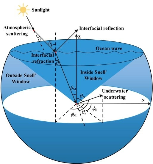
Figure 1 shows the formation mechanism of the polarization pattern induced by wavy water surfaces. Before sunlight penetrates into the water, it is scattered by the atmospheric particles first. Then, some light is reflected by the wavy water surfaces and forms the reflection polarization pattern. Some light is refracted by the wavy water surfaces, further scattered by the underwater particles, and finally forms the underwater polarization pattern. Both types of light contain lots of information.
2.1. Atmospheric Scattering
The major source of the polarization pattern induced by wavy water surfaces is the scattered skylight. To estimate if the photon exits during multiple scatterings and further calculate scattering time and underwater depth, we first describe the atmospheric radiance distribution [22]:
where is skylight radiance, and and are atmospheric zenith angles of the sun and observation, respectively. A, B, and C are values of constants, which are given by the model of Harrison and Coombes [22]. m is the mass of the atmosphere, ρ is the regression coefficient, and τ is the optical thickness of the atmosphere. is the scattering angle:
is the atmospheric solar azimuth angle and is the atmospheric observation azimuth angle. We use the Rayleigh atmosphere model to simulate atmospheric polarization patterns:
is atmospheric DOP and is atmospheric AOP, respectively.
The polarization state of the light can be described by the Stokes vector . , , , and describe the different aspects of polarized light, respectively. The calculation formula of the Stokes vector is as follows:
The ellipsoid rate is set to 0 because the skylight is mainly linearly polarized. Thus, the Stokes vector of incident light is:
2.2. Reflection and Refraction of Air–Water Interface
When the skylight reaches the wavy ocean surface, the polarization states will change because of reflection and refraction, which can be described by the Mueller matrix. For polarization patterns reflected by wavy water surfaces (Figure 2), the change of polarization state can be represented by the reflection Mueller matrix:
where and . is the zenith angle of incidence and is the zenith angle of refraction:
where and are the refraction indices of air and water, respectively.
The refraction Mueller matrix is as follows:
When the zenith angle of the incident light is 90°, the zenith angle of refracted light is
Therefore, the skylight polarization pattern is compressed into the underwater Snell’s window. Correspondingly, there exist two kinds of underwater polarization patterns: one is inside Snell’s window and the other is outside Snell’s window (Figure 3).
Considering the existence of waves on the real sea surface, we use the Cox–Munk wave model [23] to simulate ocean waves. As shown in Figure 1, in this model, the wave surface is regarded as a collection of several small surface elements, each of which is approximately a plane. The light beams reflected or refracted by each small surface element strictly follow Snell’s refraction law. Under certain water quality conditions, the slope distribution of each face element is a function of wind speed and direction. According to the wave slope distribution, the Stokes vector of the incident light in each sampling direction in the sky is calculated, respectively. Then, the weighted average of the Stokes vector of the light beam in each direction is obtained. is the atmospheric zenith angle and is the atmospheric azimuth angle. is the underwater zenith angle and is the underwater azimuth angle. If the incident light is to be observed, it must meet the following requirements:
Then, and are projected onto the XOZ and YOZ planes:
The slope of the ocean surface element is:
In order to consider the influence of wind direction, we rotate the coordinate axis to match the wind direction. The slope of the wave plane element is expressed in the new coordinate system as:
where is the included angle of wind direction with respect to the positive direction of the X-axis. The probability that the slope component of the wave surface element is [23]
The skewness coefficients (C21 and C03) and the peakedness coefficients (C40, C22, and C04) are given by the Cox–Munk wave model [23]. , . and are the root mean square values of and , respectively:
where is the wind speed. Stokes vector after incident light from each sampling direction in the sky reflected or refracted by the water surface can be expressed as:
2.3. Underwater Scattering
We calculate the scattering Mueller matrix using Mie theory. First, we need to determine the effective radius [24] of water impurity:
r is the particle radius. n(r) is particle size distribution [25,26]:
where γA and γB are distribution parameters. CA and CB are related to the concentration of oceanic particles. Based on formula (1), we can calculate the scattering number and water depth of polarization patterns. Then, using the Monte Carlo method, we can obtain the underwater multiple Mie scattering Mueller matrix:
where k is scattering time and is the rotation matrices [27]:
where is the rotation angle:
is the underwater scattering angle. It should be noted that when the depth is low, the model of polarization patterns will only need to consider surface refraction and single Rayleigh scattering of underwater particles [16]. Thus, the Monte Carlo method and underwater multiple Mie scattering Mueller matrix are not needed under this circumstance. The final Stokes vector is thus:
Then, the underwater DOP and AOP are solved and the underwater polarization pattern is obtained.
3. Results and Discussion
3.1. Polarization Patterns Reflected by Wavy Water Surfaces
The polarization patterns reflected by water surfaces under different sun positions are shown in Figure 4. The water surface is calm. The azimuth and zenith angles of observation range from 0° to 360° and from 0° to 90°, respectively. The solar azimuth angle is 0° and the solar zenith angles are 30°, 60°, and 90°, respectively. In DOP patterns, the maximum DOP (about 100%) of the water surface reflecting skylight constitutes a characteristic ring band, called the Brewster region. The angle at which light is reflected from this ring band is 53°, known as the Brewster Angle. The AOP in most regions is 90°. This is because in general, the vertical vector is stronger than the horizontal in reflection and the opposite is true in refraction. As the solar zenith angle increases, the region with the AOP of 90° decreases. When the solar zenith angle is 90°, a more regular “∞” pattern appears. At the same time, there are still neutral points in the pattern, where the DOP is zero and the AOP is distorted. The Arago and Babinet neutral points of the skylight polarization are positioned at the left and right tips of this ∞-shaped region, respectively, where the positive polarization switches to negative polarization.
Figure 5 shows the polarization pattern of wave surface reflection at different wind directions at the wind speed of 5 m/s. The wind directions are 0°, 45°, and 90°, respectively. For better analysis features, the solar zenith angle is selected as 60°. When the wind direction changes, the pattern changes in the corresponding direction. Since the direction of wave tilt is related to the wind direction, the change of wind direction will affect the reflection direction of incident light through the wave surface. However, the overall trend remains stable, proving the feasibility of using the surface reflection polarization pattern for human utilization under various wind conditions.
Figure 6 shows the simulation results of the polarization pattern of wave surface reflection at different wind speeds at a wind direction of 0°. The wind speeds are 1 m/s, 5 m/s, and 10 m/s, respectively. For better analysis features, the solar zenith angle is selected as 60°. Higher wind speeds cause larger fluctuations in the water surface, making it easier for skylights to be refracted by waves in multiple directions. At the same time, the Cox–Munk wave model has a good simulation effect under moderate wind speed. Thus, when the wind speed increases, both the DOP and AOP patterns become fuzzy and decrease regularly. However, the general distribution trend is stable.
The simulation of the proposed model is consistent with the underwater measurement of Oulu [28]. For better comparison, the simulation uses the same legend as the actual map. In the experiment, a polarization imager with an observation field of 180° was used to obtain polarization patterns reflected on the wavy water surface as shown in Figure 7. The water is calm and 10–15 m deep. The DOP and AOP patterns of reflection were measured from the vertical direction in visible light wavelength. In the experimental figure, the position of the mirrored sun is represented by a white dot, the horizon is represented by a black circle, and the noise area in the outer circle is the overexposed part. Based on the physical parameters of the experiment scene, we carry out the corresponding simulation by our model. As can be seen from the figure, the distribution law and variation trend of simulation and experimental results are consistent. The position of neutral points and relevant features are matched, which proves that it is reasonable to use the single Rayleigh scattering model and Fresnel refraction theory to describe polarization characteristics of wavy ocean surface reflection.
In order to further investigate the variation of the water surface reflection polarization pattern with respect to the solar zenith angle, we analyzed the polarization distribution on the calm water surface at different zenith angles on and perpendicular to the solar meridian. Since the AOP in most regions is 90°, we mainly explored the distribution characteristics of the DOP, as shown in Figure 8. Figure 8a is the DOP at different zenith angles on the solar meridian and Figure 8b is the DOP at different zenith angles perpendicular to the solar meridian. While on the solar meridian, the region with the higher DOP is between the observed zenith angle of 40° and 60° and has less to do with the solar zenith angle. When perpendicular to the solar meridian, the region with higher DOP is related to the solar zenith angle. When the solar zenith angle is small, the region with higher DOP is between the observed zenith angle of 40° and 60°. When the solar zenith angle is large, the region with higher DOP is between the observed zenith angle of 30° and 50°.
In this section, we study polarization patterns of wave ocean surface reflection. The influence of different sun’s positions, wind direction, and wind speed on wave surface reflection polarization patterns is discussed. The consistency of simulation and measurements proves the correctness of our model. The results show that polarization patterns reflected by the wave surface can be predicted, which is mainly related to the sun’s position, wind direction, and wind speed. The model can be used to accurately analyze the polarization characteristics of surface-reflected light and provide the theoretical basis for remote sensing.
3.2. Polarization Patterns inside Snell’s Window under Wavy Water Surfaces
The research on underwater polarization patterns inside Snell’s window is relatively mature. Thus, we mainly conduct a comparative analysis between the simulation and experiment in this section to verify the correctness of our model. The simulation of the proposed model is compared with the measurement in the Santa Barbara Channel and Hawaii [29] in visible light wavelength. The simulation uses the same legend as the actual map. In the experiment, the solar zenith angles were 77° and 88°, the water depths were 6 m and 1.5 m, the water surface wind speed was 6 m/s, and the wind direction was 0°. Figure 9 shows the quantitative analysis of underwater DOP patterns. The maximum DOP sets in the simulation were the same as that in the experiment, which were 45% and 60%. Other experimental conditions and equipment were consistent with those mentioned above. By comparing the simulation and experimental data of DOP at different zenith angles in the main plane of the sun, it can be found that the maximum DOP positions of the simulation and experiment are consistent. Figure 10 shows the quantitative analysis of underwater AOP patterns. In the quantitative analysis, the AOP simulation and experimental data of the observed zenith angle of 20° and observed azimuth angle of 90° to 270° are compared. We find that the AOP patterns are in good agreement with the measured results and the value of AOP is about 0° when the observed azimuth is 90°. In contrast, AOP patterns are more robust in general underwater environments and have better application potential [30,31]. Considering that the Cox–Munk wave model has a good simulation effect under moderate wind speed, the model in this paper has a high accuracy under moderate wind speed. Because the polarization characteristics of light are related to its propagation direction, the wave morphology has a great influence on the polarization distribution in shallow water. The proposed model is beneficial for the study of the optical transmission process of atmospheric and oceanic coupled systems.
3.3. Polarization Patterns outside Snell’s Window under Wavy Water Surfaces
Polarization patterns outside Snell’s window under the wavy water surface under different sun positions are shown in Figure 11. The wind direction is 0° and the wind speed is 5 m/s. The solar zenith angles are 0°, 30°, 60°, and 90°, respectively. The observed azimuth angles range from 0° to 360°, the observed zenith angles range from 0° to 90°, respectively, and the solar azimuth is 0°. Underwater polarization patterns inside and outside Snell’s window are continuous at the boundary. In this section, considering the two have different formation mechanisms, we separate the pattern of the inside and outside of Snell’s window and only show the polarization distribution outside Snell’s window for a better comparative analysis of relevant laws. With the increase of the solar zenith angle, the DOP increases as a whole and the position of the maximum DOP band changes further. In the AOP pattern, the AOP changes numerically and morphologically. The DOP pattern is symmetric with respect to the solar meridian and the AOP pattern is negative with respect to the solar meridian. The underwater polarization patterns outside Snell’s window have strong regularity, which are predictable and have rich information that can be used by marine organisms and even human beings.
In the experiment [29], solar zenith angles were 43°, 58°, and 61°, respectively. In the simulation, the maximum DOP was set as equal to the measurements in visible light wavelength: 38%, 35%, and 40%. The depths were 24 m, 11 m, and 17 m. The wind speed was about 6–8 m/s and the wind direction was 0°. Other experimental conditions and equipment were consistent with those mentioned above. Figure 12 is the simulation and measurement of the underwater DOP pattern outside Snell’s window. The position and morphology of the maximum DOP band of the simulation are consistent with the measurement. Figure 13 is the simulation and measurement of underwater AOP patterns outside Snell’s window. The simulation and measurement also maintain good similarity. The simulated polarization pattern and variation rule outside Snell’s window are consistent with the experimental data, which proves the correctness of the theoretical model. However, when the depth is large and the DOP is low, the consistency of simulation and measurement decreases. The lower DOP will decrease the reliability of polarization imaging and increase the image noise.
Figure 14a shows the comparison of specific values of DOP of each observed zenith angle outside Snell’s window in the main solar plane when the solar zenith angle is 58°. The results show that the trend of simulation and measured results is basically consistent. When the DOP is larger, the polarization pattern is more stable and the consistency between simulation and experiment is better. Figure 14b shows the comparison of specific values of AOP in each observed direction between simulation and experiment [32] when the solar zenith angle is 47°. Compared with the DOP, the consistency of the AOP simulation and experiment is better. This is due to the robustness of AOP for a variety of conditions, which also explains why AOP is used in current polarization navigation. The quantitative analysis and comparison of the DOP and AOP simulations and experiments further prove the reasonability of the propped model and the predictability of the underwater polarization patterns outside Snell’s window.
In this section, the polarization pattern outside Snell’s window under wavy ocean surfaces is studied. The influence of different sun’s positions on the polarization pattern outside Snell’s window under wavy ocean surfaces is discussed. The consistency of the simulation and experimental data proves the correctness of the proposed model. We find that the polarization pattern outside Snell’s window under the wavy ocean surface is predictable and mainly related to the solar position. This model can be used to analyze the polarization characteristics of Snell’s window under the wave water surface more accurately. At the same time, there are still differences between the simulation and the measured results. Poor water quality, underwater reflection, and high wind speed can also cause model failure. When the depth is large, due to the increase in scattering times and the complexity of the optical path, the simulation results of the model will be different from the measured results. However, in general, this model can predict the polarization distribution outside Snell’s window and serve underwater polarization navigation. The accuracy of the model will be further improved by experimental calibration.
4. Conclusions
Based on the Stokes vector and Mueller matrix, the model of polarization patterns induced by wavy water surface is established. We verify the correctness of the model by comparing the simulation with the experiment. The results illustrate that the polarization patterns induced by a wavy water surface are predictable under certain conditions and contain important information, which can be used by aquatic organisms and even human beings. This model can predict the polarization patterns induced by wavy water surfaces. Based on the physical model and the radiation transmission theory, the simulation accuracy is high, the speed is fast, and the polarization characteristics of the water surface can be directly reflected. It provides a theoretical basis for remote sensing, target detection, and polarization navigation. By analyzing the polarization pattern, we can obtain the ocean remote sensing information better, so as to serve for water quality monitoring, underwater particle retrieval, marine geographic exploration, and so on. For underwater target detection, we can conduct image recovery using the optical parameters calculated by the proposed model. Then, we can obtain clear underwater images and extend the underwater working distance. At the same time, the research can promote the development of polarization navigation whose precision can be improved by the calibration algorithm based on the polarization pattern. At the same time, single Rayleigh scattering is used to describe the polarization distribution in clear skies. Therefore, when the weather was poor, such as cloudy and haze, the model could not predict the polarization distribution of water reflection well. The Cox–Munk wave model only has a good simulation effect under moderate wind speed, so an increase in wind speed will also lead to the failure of the model. In addition, the performance of polarization measuring equipment, measuring methods, and water conditions and depth will also affect the consistency of the simulation and experiment. In the future, we will improve the accuracy of the model by solving the above problems.
Author Contributions
Methodology, H.C.; writing—review and editing, Q.Z., Z.W., Z.Z. and J.Q. All authors have read and agreed to the published version of the manuscript.
Funding
This research was funded by Laoshan Laboratory (LSKJ202203500), Shandong Postdoctoral Science Foundation (SDBX2023012), and Qingdao Postdoctoral Program Grant (QDBSH20230202009).
Data Availability Statement
The data that support the findings of this study are available from the corresponding author upon reasonable request.
Conflicts of Interest
The authors declare no conflict of interest.
References
- Lambrinos, D.; Möller, R.; Labhart, T.; Pfeifer, R.; Wehner, R. A mobile robot employing insect strategies for navigation. Robot. Auton. Syst. 2000, 30, 39–64. [Google Scholar] [CrossRef]
- Schwind, R. Spectral regions in which aquatic insects see reflected polarized light. J. Comp. Physiol. A 1995, 177, 439–448. [Google Scholar] [CrossRef]
- Lerner, A.; Sabbah, S.; Erlick, C.; Shashar, N. Navigation by light polarization in clear and turbid waters. Philos. Trans. R. Soc. B 2011, 366, 671–679. [Google Scholar] [CrossRef] [PubMed]
- Lynch, D.K. Snell’s window in wavy water. Appl. Opt. 2015, 54, B8–B11. [Google Scholar] [CrossRef]
- Waterman, T.H. Polarization patterns in submarine illumination. Science 1954, 120, 927–932. [Google Scholar] [CrossRef]
- Tonizzo, A.; Zhou, J.; Gilerson, A.; Twardowski, M.S.; Gray, D.J.; Arnone, R.A.; Gross, B.M.; Moshary, F.; Ahmed, S.A. Polarized light in coastal waters: Hyperspectral and multiangular analysis. Opt. Express 2009, 17, 5666–5682. [Google Scholar] [CrossRef]
- Sabbah, S.; Barta, A.; Gal, J.; Horvath, G.; Shashar, N. Experimental and theoretical study of skylight polarization transmitted through Snell’s window of a flat water surface. J. Opt. Soc. Am. A 2006, 23, 1978. [Google Scholar] [CrossRef]
- Ivanoff, A.; Waterman, T.H. Factors, mainly depth and wavelength, affecting the degree of underwater light polarization. J. Mar. Res. 1958, 16, 283–307. [Google Scholar]
- Waterman, T.H. Polarization of scattered sunlight in deep water. Deep Sea Res. 1955, 3, 426–434. [Google Scholar]
- Shashar, N.; Sabbah, S.; Cronin, T.W. Transmission of linearly polarized light in seawater: Implications for polarization signaling. J. Exp. Biol. 2004, 207, 3619–3628. [Google Scholar] [CrossRef]
- Sabbah, S.; Lerner, A.; Erlick, C.; Shashar, N. Under water polarization vision-A physical examination. Recent Res. Dev. Exp. Theor. Biol. 2005, 1, 123–176. [Google Scholar]
- Goddard, S.M.; Forward, R.B. The role of the underwater polarized light pattern, in sun compass navigation of the grass shrimp, Palaemonetes vulgaris. J. Comp. Physiol. A 1991, 169, 479–491. [Google Scholar] [CrossRef]
- Shashar, N.; Hagan, R.; Boal, J.G.; Hanlon, R.T. Cuttlefish use polarization sensitivity in predation on silvery fish. Vis. Res. 2000, 40, 71–75. [Google Scholar] [CrossRef] [PubMed]
- Waterman, T.H. Reviving a neglected celestial underwater polarization compass for aquatic animals. Biol. Rev. 2006, 81, 111–115. [Google Scholar] [CrossRef] [PubMed]
- Cartron, L.; Josef, N.; Lerner, A.; McCusker, S.D.; Darmaillacq, A.S.; Dickel, L.; Shashar, N. Polarization vision can improve object detection in turbid waters by cuttlefish. J. Exp. Mar. Biol. Ecol. 2013, 447, 80–85. [Google Scholar] [CrossRef]
- Cheng, H.; Chu, J.; Zhang, R.; Tian, L.; Gui, X. Underwater polarization patterns considering single Rayleigh scattering of water molecules. Int. J. Remote Sens. 2020, 41, 4947–4962. [Google Scholar] [CrossRef]
- Cheng, H.; Chu, J.; Zhang, R.; Tian, L.; Gui, X. Turbid underwater polarization patterns considering multiple Mie scattering of suspended particles. Photogramm. Eng. Remote Sens. 2020, 86, 737–743. [Google Scholar] [CrossRef]
- Cheng, H.; Chu, J.; Zhang, R.; Zhang, P. Simulation and measurement of the effect of various factors on underwater polarization patterns. Optik 2021, 237, 166637. [Google Scholar] [CrossRef]
- Cheng, H.; Chu, J.; Zhang, R.; Gui, X.; Tian, L. Real-time position and attitude estimation for homing and docking of an autonomous underwater vehicle based on bionic polarized optical guidance. J. Ocean Univ. China 2020, 19, 1042–1050. [Google Scholar] [CrossRef]
- Cheng, H.; Chu, J.; Chen, Y.; Liu, J.; Gong, W. Polarization-based underwater image enhancement using the neural network of Mueller matrix images. J. Mod. Opt. 2022, 69, 264–271. [Google Scholar] [CrossRef]
- Cheng, H.; Zhang, D.; Zhu, J.; Yu, H.; Chu, J. Underwater target detection utilizing polarization image fusion algorithm based on unsupervised learning and attention mechanism. Sensors 2023, 23, 5594. [Google Scholar] [CrossRef] [PubMed]
- Harrison, A.W.; Coombes, C.A. Angular distribution of clear sky short wavelength radiance. Sol. Energy 1988, 40, 57–63. [Google Scholar] [CrossRef]
- Cox, C.; Munk, W. Measurement of the roughness of the sea surface from photographs of the sun’s glitter. J. Opt. Soc. Am. 1954, 44, 838–850. [Google Scholar] [CrossRef]
- Hess, M.; Koepke, P.; Schult, I. Optical properties of aerosols and clouds: The software package OPAC. Bull. Am. Meteorol. Soc. 1998, 79, 831–844. [Google Scholar] [CrossRef]
- Risović, D. Two-component model of sea particle size distribution. Deep Sea Res. Part I 1993, 40, 1459–1473. [Google Scholar] [CrossRef]
- Risović, D.; Martinis, M. A comparative analysis of sea-particle-size distribution models. Fizika B 1995, 4, 111–120. [Google Scholar]
- You, Y.; Tonizzo, A.; Gilerson, A.A.; Cummings, M.E.; Brady, P.; Sullivan, J.M.; Twardowski, M.S.; Dierssen, H.M.; Ahmed, S.A.; Kattawar, G.W. Measurements and simulations of polarization states of underwater light in clear oceanic waters. Appl. Opt. 2011, 50, 4873–4893. [Google Scholar] [CrossRef]
- Gal, J.; Horvath, G.; Meyer-Rochow, V.B. Measurement of the reflection–polarization pattern of the flat water surface under a clear sky at sunset. Remote Sens. Environ. 2001, 76, 103–111. [Google Scholar] [CrossRef]
- Bhandari, P.; Voss, K.J.; Logan, L.; Twardowski, M. The variation of the polarized downwelling radiance distribution with depth in the coastal and clear ocean. J. Geophys. Res.-Ocean. 2011, 116, C00H10. [Google Scholar] [CrossRef]
- Cheng, H.; Yu, S.; Yu, H.; Zhu, J.; Chu, J. Bioinspired underwater navigation using polarization patterns within Snell’s window. China Ocean Eng. 2023, 37, 628–636. [Google Scholar] [CrossRef]
- Cheng, H.; Chen, Q.; Zeng, X.; Yuan, H.; Zhang, L. The polarized light field enables underwater unmanned vehicle bionic autonomous navigation and automatic control. J. Mar. Sci. Eng. 2023, 11, 1603. [Google Scholar] [CrossRef]
- Powell, S.B.; Garnett, R.; Marshall, J.; Rizk, C.; Gruev, V. Bioinspired polarization vision enables underwater geolocalization. Sci. Adv. 2018, 4, eaao6841. [Google Scholar] [CrossRef] [PubMed]
Figure 1.
The formation mechanism of the polarization pattern induced by wavy water surfaces.

Figure 2.
Forming process of polarization patterns reflected by wavy water surfaces.

Figure 3.
Mechanism of Snell’s window formation.

Figure 4.
Simulations of DOP (a) and AOP (b) patterns reflected by water surfaces at different sun positions.
Figure 4.
Simulations of DOP (a) and AOP (b) patterns reflected by water surfaces at different sun positions.

Figure 5.
Simulations of DOP (a) and AOP (b) patterns reflected by water surfaces at different wind directions.
Figure 5.
Simulations of DOP (a) and AOP (b) patterns reflected by water surfaces at different wind directions.

Figure 6.
Simulations of DOP (a) and AOP (b) patterns reflected by water surfaces at different wind speeds.
Figure 6.
Simulations of DOP (a) and AOP (b) patterns reflected by water surfaces at different wind speeds.

Figure 7.
Simulation and measurement [28] of DOP (a) and AOP (b) patterns reflected by water surfaces.
Figure 7.
Simulation and measurement [28] of DOP (a) and AOP (b) patterns reflected by water surfaces.

Figure 8.
Numerical comparison of DOP reflected by water surfaces. (a) The DOP at different zenith angles on the solar meridian; (b) The DOP at different zenith angles perpendicular to the solar meridian.
Figure 8.
Numerical comparison of DOP reflected by water surfaces. (a) The DOP at different zenith angles on the solar meridian; (b) The DOP at different zenith angles perpendicular to the solar meridian.

Figure 9.
Comparative analysis of DOP patterns under wave water inside Snell’s window when the solar zenith angle is 77° (a) and 88° (b).
Figure 9.
Comparative analysis of DOP patterns under wave water inside Snell’s window when the solar zenith angle is 77° (a) and 88° (b).

Figure 10.
Comparative analysis of AOP patterns under wave water inside Snell’s window when the solar zenith angle is 77° (a) and 88° (b).
Figure 10.
Comparative analysis of AOP patterns under wave water inside Snell’s window when the solar zenith angle is 77° (a) and 88° (b).

Figure 11.
Simulations of underwater DOP (a) and AOP (b) patterns outside Snell’s window.

Figure 12.
Simulation (a) and measurement (b) of underwater DOP patterns outside Snell’s window.

Figure 13.
Simulation (a) and measurement (b) of underwater AOP patterns outside Snell’s window.

Figure 14.
Simulation and measurement of underwater DOP and AOP outside Snell’s window. (a) The comparison of specific values of DOP; (b) The comparison of specific values of AOP.
Figure 14.
Simulation and measurement of underwater DOP and AOP outside Snell’s window. (a) The comparison of specific values of DOP; (b) The comparison of specific values of AOP.

Disclaimer/Publisher’s Note: The statements, opinions and data contained in all publications are solely those of the individual author(s) and contributor(s) and not of MDPI and/or the editor(s). MDPI and/or the editor(s) disclaim responsibility for any injury to people or property resulting from any ideas, methods, instructions or products referred to in the content. |
© 2023 by the authors. Licensee MDPI, Basel, Switzerland. This article is an open access article distributed under the terms and conditions of the Creative Commons Attribution (CC BY) license (https://creativecommons.org/licenses/by/4.0/).
Share and Cite
MDPI and ACS Style
Cheng, H.; Zhang, Q.; Wan, Z.; Zhang, Z.; Qin, J. Study on the Polarization Pattern Induced by Wavy Water Surfaces. Remote Sens. 2023, 15, 4565. https://doi.org/10.3390/rs15184565
AMA Style
Cheng H, Zhang Q, Wan Z, Zhang Z, Qin J. Study on the Polarization Pattern Induced by Wavy Water Surfaces. Remote Sensing. 2023; 15(18):4565. https://doi.org/10.3390/rs15184565
Chicago/Turabian StyleCheng, Haoyuan, Qianli Zhang, Zhenhua Wan, Zhongyuan Zhang, and Jin Qin. 2023. "Study on the Polarization Pattern Induced by Wavy Water Surfaces" Remote Sensing 15, no. 18: 4565. https://doi.org/10.3390/rs15184565
Note that from the first issue of 2016, this journal uses article numbers instead of page numbers. See further details here.