Impact of Atmospheric Correction on Classification and Quantification of Seagrass Density from WorldView-2 Imagery

Abstract

Mapping the seagrass distribution and density in the underwater landscape can improve global Blue Carbon estimates. However, atmospheric absorption and scattering introduce errors in space-based sensors’ retrieval of sea surface reflectance, affecting seagrass presence, density, and above-ground carbon (AGC_seagrass) estimates. This study assessed atmospheric correction’s impact on mapping seagrass using WorldView-2 satellite imagery from Saint Joseph Bay, Saint George Sound, and Keaton Beach in Florida, USA. Coincident in situ measurements of water-leaving radiance (L_w), optical properties, and seagrass leaf area index (LAI) were collected. Seagrass classification and the retrieval of LAI were compared after empirical line height (ELH) and dark-object subtraction (DOS) methods were used for atmospheric correction. DOS left residual brightness in the blue and green bands but had minimal impact on the seagrass classification accuracy. However, the brighter reflectance values reduced LAI retrievals by up to 50% compared to ELH-corrected images and ground-based observations. This study offers a potential correction for LAI underestimation due to incomplete atmospheric correction, enhancing the retrieval of seagrass density and above-ground Blue Carbon from WorldView-2 imagery without in situ observations for accurate atmospheric interference correction.

1. Introduction

Seagrasses represent the greatest data gap in Blue Carbon habitat mapping, with their spatial extent largely under-represented in the Blue Carbon inventories for Canada, Mexico, and the United States [1]. This under-representation is due to a combination of fundamental uncertainties about the true extent and density of seagrass meadows, as well as the logistical and labor challenges involved in the ground-based mapping of submerged seagrass populations, many of which are located in remote coastal areas [2]. Remote sensing imagery obtained from air- and space-borne sensors can quantify seagrass and other benthic ecosystems, and the ability to remotely quantify seagrass meadows has been greatly enhanced by high-spatial-resolution (≤30 m) space-based sensors such as Landsat, IKONOS, Quickbird-2, RapidEye, WorldView-2 and -3, and Sentinel-2 [3,4,5,6,7,8,9,10,11,12].

Space-based observations benefit from the radiometric calibration provided by most satellite-based sensors, allowing the generation of optically consistent remote sensing reflectance (R_rs, sr⁻¹) products that account for differences in solar illumination across time and space. This optical consistency is essential for change detection and the creation of climate-quality data records [13]. Automated pixel-based classification, which also requires optical consistency, enables more precise estimates of spatial cover compared to manually delineated polygons obtained from aerial imagery [14,15]. It also facilitates the calculation of landscape-scale metrics, such as patch shape, area, and separation, which are critical for determining changes in the shape of seagrass meadows resulting from the loss, gain, fragmentation, and/or merging of vegetated patches [16].

The automated classification of imagery is typically achieved via supervised methods, often referred to as object-based image analysis (OBIA), which utilizes pre-determined sections of the image as a training dataset. The use of complex machine learning techniques to separate seagrass from other benthic classes based on spectral characteristics is in its infancy, but a deep convolutional neural network (DCNN) has been shown to achieve high accuracies for images generated by a variety of satellite-based sensors, including RapidEye, WorldView-2 [3], and Landsat-5, -7, and 8 [5], with less computational complexity compared to other approaches [17,18].

The retrieval of the above-ground carbon biomass of seagrass (AGC_seagrass) is a crucial step in utilizing satellite imagery for Blue Carbon mapping. The above-ground vegetation density quantified from space can be linked to ecologically relevant properties, including standing carbon biomass, ecosystem productivity, and Blue Carbon stocks ([19] and references therein). These estimates are critical for understanding the carbon budget of coastal oceans and can help quantify the economic value of these coastal ecosystems, which is estimated to be between USD 5000 and USD 19,000 per hectare annually [20,21].

Methods to retrieve aquatic biomass from satellites have followed two pathways. The first pathway incorporates radiative transfer modeling to remove the effects of the overlying water column to provide top-of-canopy reflectance, from which the seagrass density is then derived based on local in situ relationships between canopy reflectance and the leaf area index (LAI) [22,23]. AGC_seagrass is then calculated from LAI using a series of transfer coefficients [24,25,26]. The second pathway uses locally derived, image-specific empirical relationships between sea surface reflectance properties above seagrass meadows and percent cover or above-ground carbon (AGC_seagrass [10,11]), which are not easily transferred to other images. By retrieving top-of-canopy reflectance, the radiative transfer approach provides a more general solution that accounts for differences in water column depth and optical properties that can obscure the estimation of LAI and standing biomass. This correction is particularly important for improving seagrass mapping in optically complex waters [12] and remote locations, where ground data can be difficult to obtain.

If in situ observations of water-leaving radiances coincident with the satellite overpass are available, then absorption and scattering by the atmosphere can be corrected using the empirical line height (ELH) method [27]. However, the availability of in situ calibration target measurements is rare, and it is therefore common to employ a correction procedure, such as a dark-object subtraction (DOS [28,29]). As with the ELH approach, complex radiative transfer correction methods, such as Fast Line-of-sight Atmospheric Analysis of Hypercubes (FLAASH) and Atmospheric and Topographic Correction (ATCOR [30]), require numerous input terms, including atmosphere optical thickness, that can be difficult to parameterize for high-resolution imagery at these scales. Comparisons between in situ water-leaving radiance and satellite retrievals processed through various atmospheric correction methods typically leave residual brightness in all bands, especially the blue region of the spectrum, across multiple sensors used for seagrass classification, including Landsat, Sentinel-2, WorldView-2, and RapidEye [3,11,30,31,32,33,34]. However, those studies did not routinely quantify the impact of the AC error on the quantification of the seagrass distribution or density across the submarine landscape.

Here, we explored the extent to which accuracy and precision in AC impact the ability to retrieve the seagrass distribution and density from WorldView-2 multispectral images from the Gulf Coast of Florida. Our primary goal was to develop a robust algorithm for seagrass classification and density determination that provides a path for the routine, accurate mapping of submerged aquatic vegetation (SAV) across the submarine landscape. The future ability to exploit the growing archive of images from orbiting sensors to quantify important changes in coastal environments requires us to assess the impacts of incomplete atmospheric correction on our classification and quantification algorithms.

2. Methods

2.1. Study Sites

We focused on three sites located along the Florida Gulf Coast, USA (Figure 1). Full characterization of the water column optical properties and quantification of seagrass abundance were undertaken at stations across all study sites (Figure 2) between 18 and 26 May 2010 near Keaton Beach, 1 and 9 November 2010 in Saint Joseph Bay, and 24 April and 5 May 2012 in Saint George Sound, coincident with the scheduled image acquisition at each site.

Saint Joseph Bay is the only embayment in the eastern Gulf of Mexico not directly influenced by riverine input. It does, however, receive water rich in colored dissolved organic matter (CDOM) from the Gulf County Canal, constructed in 1938, which links the Intracoastal Waterway to the bay [35]. At Port Saint Joe, seagrass meadows are extensively distributed in shallow nearshore waters (<2 m depth) throughout the bay, especially at the southern (closed) end, and their distribution has been temporally stable from 1990 to 2020 [5].

Saint George Sound forms the eastern portion of the Apalachicola Bay estuary/lagoon system, which is heavily influenced by the Apalachicola River, receiving discharge from agricultural, industrial, and municipal activities in the 50,000 km² Apalachicola–Flint–Chattahoochee River Basin. Seagrasses are abundant in the shallow, quiescent waters along the mainland coast of the eastern portion of Saint George Sound between Carrabelle and St. Teresa and in the lee of Dog Island Reef (Figure 2B) that separates the southern boundary of St. George Sound from the northern Gulf of Mexico. Seagrasses are absent from the highly turbid waters in the western portion of Apalachicola Bay and in the much smaller Alligator Harbor at the east end.

Keaton Beach is located at the northern end of the Big Bend Seagrass Aquatic Preserve, which encompasses the second-largest contiguous area of seagrass habitat in the eastern Gulf of Mexico [36]. Unlike St. Joseph’s Bay and St. George Sound, in which seagrass meadows are confined to shallow embayments or protected lagoon waters, the seagrass meadows along Keaton Beach inhabit the open Gulf Coast to depths extending to the 3 m isobath. The coastal waters of Keaton Beach are influenced by CDOM-rich but oligotrophic discharge from the Steinhatchee River, a short river derived from the relatively undeveloped watershed dominated by cypress swamps, titi swamps, peat bogs [37], and other non-point sources along this section of the coast.

2.2. Measurement of Water Column Optical Properties and In Situ R_rs

All symbols and definitions described in this and following sections are summarized in

Table 1. Summary of symbols, their definitions, and their dimensions.

Symbol	Definition	Dimensions
Basic parameters
Rrs(DOS)	Remote sensing reflectance from DOS atmospheric correction	sr−1
Rrs(ELH)	Remote sensing reflectance from ELH atmospheric correction	sr−1
Ed(λ)	Spectral downwelling irradiance	W m−2
Eu(λ)	Spectral upwelling irradiance	W m−2
Lu(λ)	Spectral upwelling radiance	W m−2 sr−1 nm−1
Lw(λ)	Spectral water-leaving radiance	W m−2 sr−1 nm−1
zb	Depth of water column from digital elevation map	m
z	Depth of the water column corrected for canopy height and tidal state	m
LAI	Leaf area index	m2 leaf m−2 ground
AGCseagrass	Above-ground seagrass carbon	g
Inherent optical properties of the water column (IOPs)
ap	Absorption by particulate material (algal + sediment + detritus)	m−1
an	Absorption by non-pigmented particulate material	m−1
ag	Absorption by CDOM	m−1
apg	Absorption by particulate and CDOM	m−1
bp	Scattering by particulate material	m−1
bbp	Backscattering by particulate material	m−1
cpg	Beam attenuation coefficient	m−1
Apparent optical properties of the water column (AOPs)
Kd(λ)	Spectral downwelling diffuse water column attenuation coefficient	m−1
KLu (λ)	Spectral upwelling diffuse attenuation coefficient	m−1
Rb(λ)	Spectral benthic reflectance	dimensionless

. The inherent optical properties (IOPs) of spectral absorption (a, m⁻¹) and beam attenuation (c, m⁻¹) were measured at nine channels (412, 440, 488, 510, 532, 555, 650, 676, 715 nm) using an ac-9 Plus (Sea-Bird Instruments) deployed 1 m below the surface at each station. The ac-9 data were corrected for ambient temperature, salinity, and scattering according to Method 3 [38] using a Conductivity, Temperature, and Depth (CTD) sensor incorporated into the ac-9 package. Scattering correction was performed using data from a Hydroscat-6P series 300 (HOBI Labs, Inc.) deployed alongside the ac-9. All data processing of the Hydroscat-6 data was undertaken in accordance with manufacturers’ protocols, including the σ correction for highly scattering waters. Attenuation and absorption by particles plus CDOM (c_pg, a_pg) were calculated by subtracting the absorption and scattering of pure water [39] from the temperature- and salinity-corrected data. The total spectral scattering coefficient (b_p(λ),m⁻¹) was calculated as:

$$b_{\mathrm{p}}\left(\lambda \right)=c_{\mathrm{p}\mathrm{g}}\left(\lambda \right)-a_{\mathrm{p}\mathrm{g}}\left(\lambda \right)$$

(1)

under the assumption that CDOM did not contribute to scattering.

A HyperPro profiling radiometer (SatLantic Instruments) and hyperspectral tethered spectroradiometer buoy (HTSRB, SatLantic Instruments) were floated in tandem at each station to measure downwelling spectral irradiance (E_s(λ,0⁺)) above the sea surface and upwelling spectral radiances (L_u(λ)) at 0.21 m and 0.65 m, respectively, beneath the sea surface. The diffuse attenuation coefficient for upwelling radiance was calculated as:

$$K_{\mathrm{L}\mathrm{u}}\left(\lambda \right)=-\frac{1}{∆z}\mathrm{I}\mathrm{n}\frac{L_{\mathrm{u}}(\lambda ,0.65\mathrm{m})}{L_{\mathrm{u}}(\lambda ,0.21\mathrm{m})}$$

(2)

where Δz was the difference in depth (0.44 m) between the sensors placed at 0.21 and 0.65 m. The water-leaving radiance (L_w(λ)) was calculated by propagating L_u(λ) to the surface using K_Lu(λ) and transmitting it across the air–water interface:

$$L_{\mathrm{w}}\left(\mathsf{\lambda }\right)=\frac{t_{\mathrm{u}}{L}_{\mathrm{u}}\left(l,0.21\right)}{\mathrm{e}\mathrm{x}\mathrm{p}\left[{-0.21K}_{\mathrm{L}\mathrm{u}}\left(\lambda \right)\right]}$$

(3)

where ${\tau }_{\mathrm{u}}$ (=0.54,) represented the fraction of upwelling radiance transmitted upward across the water–air interface of a flat ocean [40,41]. In situ remotely sensed reflectances (R_rs(λ), sr⁻¹) were then calculated as:

$$R_{\mathrm{r}\mathrm{s}}(\lambda )=\frac{L_{\mathrm{w}}\left(\lambda \right)}{E_{\mathrm{s}}(\lambda ,0+)}$$

(4)

R_rs(λ) was then averaged to match the multispectral wavelength bins of the WorldView-2 sensor, using the response functions provided by DigitalGlobe (

Table 2. WorldView-2 spectral center wavelengths and band edges.

Band Name	Center Wavelength (nm) (Lower and Upper Band Edges)
MS1 (NIR1)	835 (770–895)
MS2 (Red)	660 (630–690)
MS3 (Green)	545 (510–580)
MS4 (Blue)	480 (450–510)
MS5 (Red edge)	725 (705–745)
MS6 (Yellow)	605 (585–625)
MS7 (Coastal)	425 (440–450)
MS8 (NIR 2)	950 (860–1040)

).

2.3. In Situ Seagrass Density

Direct counts of Thalassia testudinum (turtle grass), Halodule wrightii (shoal grass), and Syringodium filiforme (manatee grass) shoots were performed by SCUBA divers using 20 to 30 quadrats (0.04 m²) randomly located within a 20 m radius at optically shallow water stations at each site (Figure 2). Halophila spp. (paddlegrass) and Ruppia maritima (widgeon grass) were not present in any of the quadrats. One shoot of each species present was collected from each quadrat for subsequent measurement of total leaf length, leaf width, and number of leaves per shoot and determination of leaf area index (LAI = $\frac{\mathrm{s}\mathrm{h}\mathrm{o}\mathrm{o}\mathrm{t}\mathrm{s}}{{\mathrm{m}}^2 \mathrm{s}\mathrm{e}\mathrm{a}\mathrm{f}\mathrm{l}\mathrm{o}\mathrm{o}\mathrm{r}}\times \frac{{\mathrm{m}}^2 \mathrm{l}\mathrm{e}\mathrm{a}\mathrm{f} \mathrm{a}\mathrm{r}\mathrm{e}\mathrm{a}}{\mathrm{s}\mathrm{h}\mathrm{o}\mathrm{o}\mathrm{t}}$). The LAI of Syringodium filiforme was calculated using the diameter of the cylindrical leaves for leaf width.

2.4. Top-of-Canopy Reflectance Measurements

Downwelling (E_d(λ,z)) and upwelling (E_u(λ,z)) spectral irradiances were measured at the top of the seagrass canopy and at 15 cm above the bare sediment at ~10 randomly selected spots at each station using our Diver-Operated Benthic Bio-Optical Spectrometer (DOBBS), a three-channel radiometer (HR-3, HOBI Labs, Inc.) configured for portable in situ operation by a diver. Instrument spectra (nominally 0.3 nm resolution) were interpolated to 1 nm with a cubic spline and smoothed using a 21 nm running average. Spectral reflectance (R_b(λ), dimensionless) of the seagrass canopy or bare substrate was calculated as $\frac{E_{\mathrm{u}}\left(\mathsf{\lambda },z\right)}{E_{\mathrm{d}}\left(\mathsf{\lambda },z\right)}$. R_b(green) was then calculated by averaging R_b(λ) across the WorldView-2 green band (511 to 581 nm). The mean and standard error of R_b(green) were calculated for each station.

The top-of-canopy reflectance measurements were paired with coincident LAI measurements (Section 2.3) to generate a regression model that could be used with top-of-canopy reflectance retrieved from R_rs (Section 2.6.3) to estimate LAI from the images.

2.5. Satellite Data

The WorldView-2 satellite imaging system operated by Maxar Technologies, Inc. (formerly DigitalGlobe) was tasked to obtain multispectral images of Keaton Beach, Saint Joseph Bay, and Saint George Sound. Tasking information included the optimal geometry relative to the target to minimize direct solar reflectance (sunglint) and local cloud cover. Image collection took place on 20 May 2010 (Keaton Beach), 14 November 2010 (Saint Joseph Bay), and 27 April 2012 (Saint George Sound,

Table 3. WorldView-2 image information for all three sites. Data from NOAA tide stations were used to correct mean lower low water levels to water depth at the time of the image collection.

Date	Location	MAXAR Image ID	View Angle (Degrees Off-Nadir)	Ground Resolution (m)	Sun Elevation	NOAA Tide Station ID
20 May 2010	Keaton Beach	10300100045A9500	36.7°	3	68.8°	8727695
14 Nov 2010	Saint Joseph Bay	103001000897AC00	15.6°	2	40.5°	8728912
27 Apr 2012	Saint George Sound	10300100184AB500	35.4°	3	67.6°	8728360

and Figure 2). Ground resolution, which depended on the view angle required to minimize glint, varied from 2 m at Saint Joseph Bay to 3 m at both Keaton Beach and Saint George Sound (Table 3).

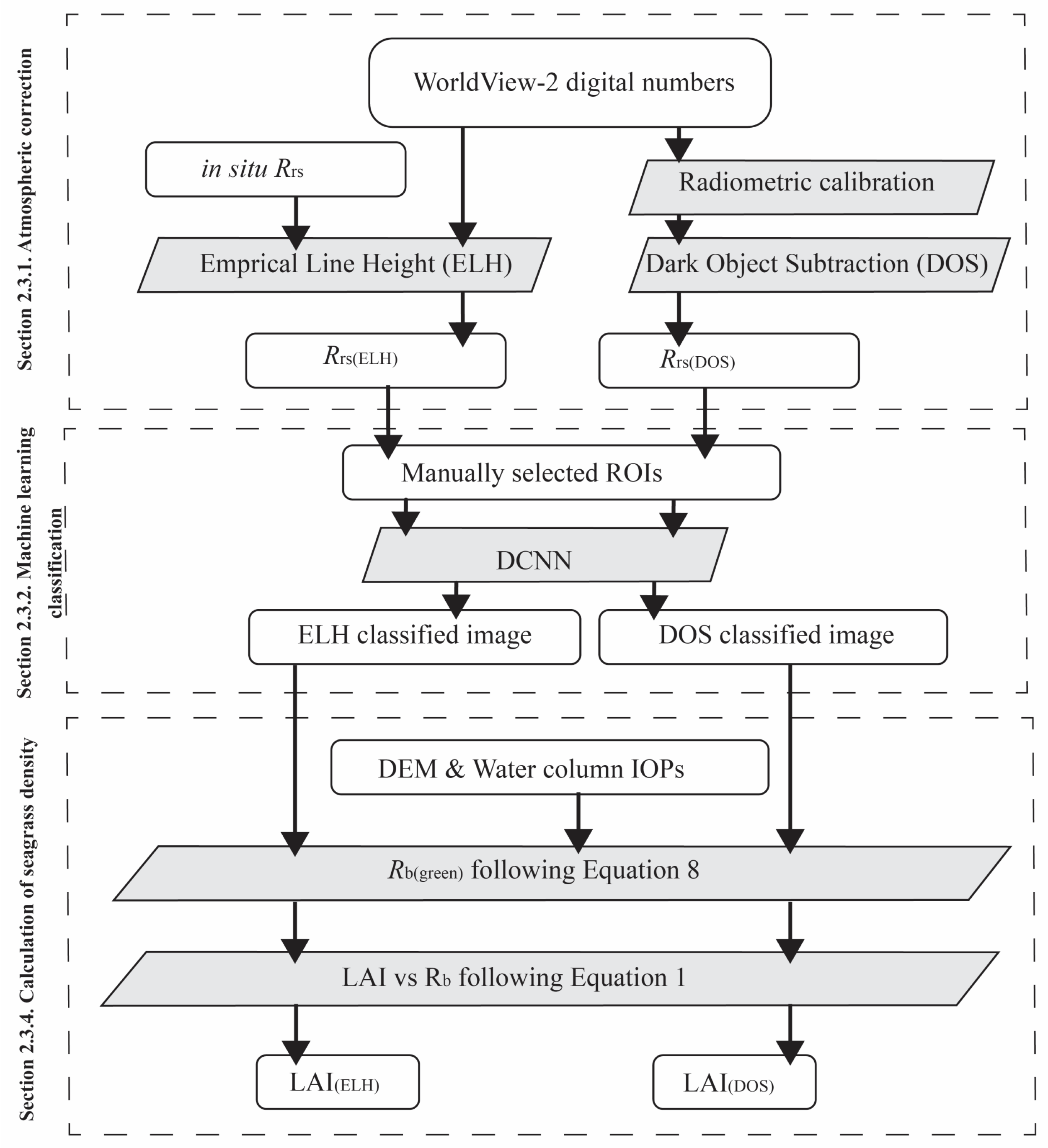
2.6. Data Processing

2.6.1. Atmospheric Correction

Raw, top-of-atmosphere digital values (Level 1b data product) were converted to sea surface reflectance (R_rs) for each image using two atmospheric correction methods (Figure 3). The ELH method incorporates both radiometric calibration and atmospheric correction into a single step [27,42] using in situ observations of R_rs collected coincidently with the satellite overpass (Section 2.2) at “optically deep” stations where the geometric water depth exceeded the depth of the 10% isolume, defined by the diffuse attenuation coefficient K_d. These in situ reflectance values were regressed against the average digital value obtained from a 4 × 4 pixel array extracted from the image corresponding to the location of each station to create R_rs gains (slopes) and offsets (intercepts) for all bands that were subsequently applied to the entire image. Accuracy of the in situ L_w(λ) measurements was validated against HydroLight [43] simulations parameterized with IOP data from the ac-9 and Hydroscat-6 measurements at those stations (Section 2.2). R_rs generated from this method will be referred to in the text as R_rs(ELH) (Figure 3).

Atmospheric correction was also undertaken using the DOS approach [44]. Radiometric calibration and DOS were performed on each image in separate steps, as described in Coffer et al. [3], using radiometric calibration coefficients from Kuester [45]. The red-edge band (MS5, Table 2) was used as the DOS reference band because radiometric calibration of the near-infrared (NIR) bands using coefficients provided by Maxar frequently yielded negative radiances over dark water targets before atmospheric correction, preventing their use for DOS [3]. Inland water pixels were excluded from the red-edge analysis by masking the land area using a shapefile of the coastline [46]. A normalized difference water index (NDWI) was then applied to remove any remaining shoreline pixels [47]. The median of the red-edge R_rs values was then computed from the optically darkest 5% of the remaining water pixels. We assumed that half of the red-edge radiance emanating from the dark pixels represented atmospheric contamination [3], while the remainder represented true water-leaving radiances. The scattering factor (s) was computed as

$$\sigma ={\lambda }_{rededge}^{4.75}\times {\alpha }_{rededge}$$

(5)

where α is anchored to the correction at the red edge at 0.5. The wavelength-dependent Rayleigh exponent was set to 4.75 [3]. The scattering factor was then applied to the center wavelength of each band to compute the correction factor (η_band), which was subtracted from the band-specific R_rs for all pixels in the scene:

$${\eta }_{\mathrm{b}\mathrm{a}\mathrm{n}\mathrm{d}}=\frac{\sigma }{{\lambda }_{rededge}^{4.75}}$$

(6)

The radiometrically calibrated and atmospherically corrected R_rs values generated from this method are identified below as R_rs(DOS) (Figure 3).

2.6.2. Machine Learning Supervised Classification

A deep convolutional neural network (DCNN, [17]) previously used to separate seagrass from other targets in imagery from WorldView-2 and RapidEye [3] sensors was used to classify the R_rs(ELH) and R_rs(DOS) images. Four classes were identified at all sites: (i) optically deep water, in which the bottom type was unidentifiable, (ii) optically shallow submerged sand, (iii) submerged seagrass, and (iv) dry land consisting of natural vegetation and human development. A fifth class of emergent intertidal sand covered with benthic algal film was identified only in Saint Joseph Bay. The DCNN was trained using representative patches (rectangular polygons) of each class, referred to as regions of interest (ROIs), identified in each image through a combination of local knowledge and visual confirmation (Figure 2). ROIs were split into training and testing subsets for the DCNN model, and a subsequent patch size of 3 × 3 pixels was extracted from the ROIs to use as training samples. The DCNN consisted of a sequential model, or linear stack, of six layers. The first layer was a convolutional layer consisting of 32 filters with a kernel size of 1 × 1 × 8 (containing 1 pixel and 8 channels), followed by a rectified linear activation function. Next, a dropout layer randomly set 1% of the outputs from the first layer to zero. The second convolutional layer consisted of 16 filters with a kernel size of 3 × 3 × 32 pixels, again, followed by a rectified linear activation function. Then, another 1% dropout layer was added before flattening the model. Finally, a dense layer with a SoftMax activation function was used to compute pixel-based probabilities for each class [48]. This DCNN model was trained for 500 epochs, where an epoch represented the point at which all training data have been processed one time, using a batch size of 256. Once trained, the model was applied across the entire image to classify all pixels, resulting in separately classified images for R_rs(ELH) and R_rs(DOS) values.

2.6.3. Calculation of Seagrass Density

R_rs(ELH) and R_rs(DOS) values were used to generate benthic reflectance at the top of the seagrass canopy in the green band (R_b(green)) [22,23]:

$$R_{\mathrm{b}}(\mathrm{g}\mathrm{r}\mathrm{e}\mathrm{e}\mathrm{n})=\frac{R_{\mathrm{r}\mathrm{s}}\left(\mathrm{g}\mathrm{r}\mathrm{e}\mathrm{e}\mathrm{n}\right)Q_{\mathrm{b}}}{{\tau }_{\mathrm{u}}}\frac{exp\left[\overline{{-K}_{\mathrm{l}\mathrm{u}}\left(z_{\mathrm{b}}\right)}{z}_{\mathrm{b}}\right]}{exp\left(-K_{\mathrm{d}}{z}_{\mathrm{b}}\right)}$$

(7)

where R_rs(green) represents either R_rs(ELH) or R_rs(DOS) values from band MS3 (green, centered at 545 nm). Water depth (z_b) was extracted from NOAA’s Continuously Updated Digital Elevation Model [49] at 1 m horizontal resolution and resampled to match the grid dimensions and spatial resolution of the satellite imagery (2 to 3 m) using ArcGIS Pro. The resulting digital elevation models (DEM) for all sites were then used along with local tide predictions (Table 1) to calculate water depth across each scene at the times of WorldView-2 image acquisition. Downwelling diffuse attenuation (K_d) and depth-averaged upwelling radiance attenuation [$\overline{{-K}_{\mathrm{l}\mathrm{u}}\left(z_{\mathrm{b}}\right)}]$ coefficients were modeled using Hydrolight (© C. Mobley, Sequoia Scientific) parameterized with inherent optical properties (IOPs) measured in situ. Q_b represents the ratio of E_u to L_u at the base of the water column produced by the reflectance of E_d from the sea floor, which was assumed to be π for a Lambertian bottom boundary. The relative transmittance of L_u through the water–air interface (τ_u) was approximated as 0.54 [40]. Leaf area index was determined by linear regression of R_b(green) against direct shoot counts made at in situ stations distributed across each scene. AGC_seagrass was estimated from LAI using a series of transfer coefficients for fresh weight (Equation (8)), dry weight (Equation (9) [25,26]), and organic carbon (Equation (10) [24]).

Above-ground Fresh Wt (g FW) = 500 (g m⁻² leaf) × LAI (m² leaf m⁻² seabed)

(8)

Above-ground Dry Wt (g DW) = fresh wt × 0.2 (g DW g⁻¹ FW)

(9)

Above-ground seagrass carbon stock (g C) = dry wt (g DW) × 0.35 (g C g⁻¹ DW)

(10)

2.7. Statistical Analysis

2.7.1. Comparison of Atmospherically Corrected R_rs Values

R_rs(ELH) and R_rs(DOS) values at 400 randomly generated points were selected across each study site for comparison. Points were generated using the “create random points” tool in ArcGIS Pro across all marine targets to collect a range of R_rs values. R_rs(ELH) and R_rs(DOS) for each band were extracted from these points and subjected to linear regression. Differences in the band-specific relationships between R_rs(ELH) and R_rs(DOS) among the three sites were evaluated using Analysis of Covariance (ANCOVA).

2.7.2. Comparison of In Situ and Retrieved LAI

Direct comparisons of in situ and satellite-retrieved LAI are challenging due to the small-scale spatial heterogeneity found in seagrass meadows, where quadrat-scale LAI measured using a 0.04 m² quadrat can range from 0 to 4 m² m⁻² within the 3 m footprint of the WV-2 pixel. In order to determine whether in situ and satellite-derived LAI values were statistically similar, we extracted LAI from image pixels within a 20 m radius of our in situ seagrass stations using the “create buffer tool” in ArcGIS Pro (Figure 2). Box-and-whisker plots were generated to illustrate similarities in mean, median, and data ranges. Statistical similarity between in situ LAI calculated from direct quadrat counts (Section 2.3) and remotely detected LAI was determined via a non-parametric Kruskal–Wallis test [50] followed by a pairwise Mann–Whitney U-test [51], run using the SciPy statistical package [52].

3. Results

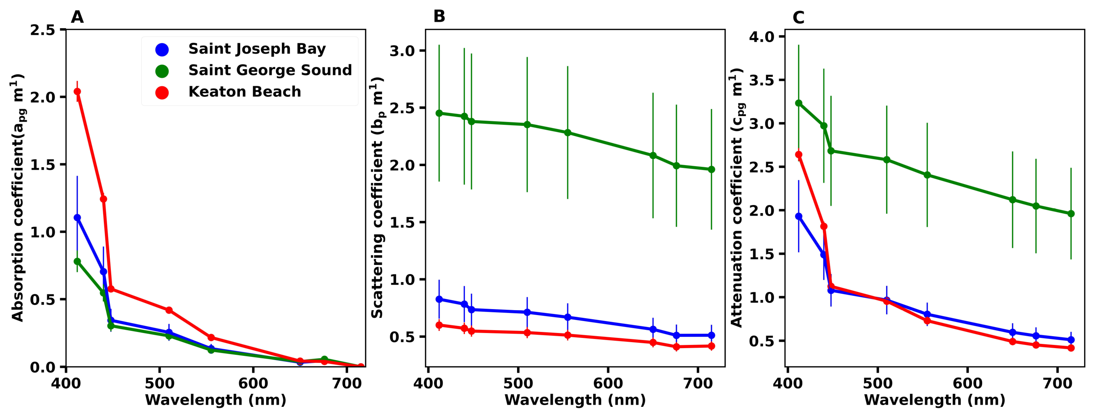
3.1. Water Column Optical Properties

The water column at all three sites consisted of optically complex Case 2 waters, with high absorption and/or scattering dominated by a combination of non-algal particles and CDOM. Keaton Beach had the highest a_pg; values at 412 and 443 nm were twice those observed at the other sites (Figure 4A). The comparatively low contribution of b_p to c_pg (Figure 4B,C) at Keaton Beach indicates that the a_pg was dominated by CDOM and not high levels of phytoplankton or other particles. Saint Joseph Bay and Saint George Sound had similar values of a_pg (Figure 4A). However, the b_p in Saint George Sound was three times higher than that observed at Saint Joseph Bay and accounted for 75% of the c_pg, suggesting a high load of non-algal particles in this lagoon fed by the Apalachicola River (Figure 5B). There was a high degree of variation in the b_p across Saint George Sound, with lower b_p and c_pg observed offshore near Dog Island Reef. In Saint Joseph Bay, both a_pg and b_p contributed equally to light attenuation. Based on the optical properties, the depth of the 10% isolume, which we used to define the limit for optically shallow water and which often corresponds to the lower limit of seagrass colonization [53,54], was 0.9 m in Saint George Sound, 2.1 m at Keaton Beach, and 2.3 m in Saint Joseph Bay.

3.2. Comparison of Remote Sensing Reflectance between Atmospheric Correction Methods

R_rs(DOS) was higher than R_rs(ELH) across all bands at all three sites, especially in bands MS7 (425 nm) and MS4 (480 nm), where R_rs(DOS) was an order of magnitude higher than R_rs(ELH) (Figure 5A,B). The relationship between R_rs(DOS) and R_rs(ELH) was positive and linear in all bands and sites, except for Keaton Beach, where we found a negative, albeit linear, relationship between R_rs(ELH) and R_rs(DOS) (Figure 5A 425 nm,

Table 4. Slope (95% confidence intervals) of the regression between R_rs(ELH) and R_rs(DOS) for each band and site.

Band	Saint Joseph Bay	Saint George Sound	Keaton Beach
MS7: 425 nm	1.29 (1.26–1.33)	2.75 (2.72–2.78)	−13.76 (−14.2–−13.29)
MS4: 480 nm	1.49 (1.48–1.50)	1.96 (1.93–1.98)	3.89 (3.68–3.95)
MS3: 545 nm	1.272 (1.268–1.275)	1.298 (1.286–1.309)	0.916 (0.893–0.940)
MS6: 605 nm	0.92 (0.915–0.922)	1.199 (1.19–1.21)	1.15 (1.09–1.22)
MS2: 660 nm	0.86 (0.863–0.852)	1.365 (1.35–1.37)	2.314 (2.26–2.37)
MS5: 725 nm	1.49 (1.47–1.5)	1.926 (1.92–1.93)	1.238 (1.21–1.26)

). Overall, the Keaton Beach image was darker than both Saint Joseph’s Bay and Saint George Sound images in bands MS7, 4, and 3 in both ELH and DOS corrections (Figure 5A–C). R_rs(DOS) was more divergent from R_rs(ELH) (slopes > 1) in the yellow (MS6) and red (MS2) bands (Table 4 and Figure 5D,E) at Keaton Beach and Saint George Sound relative to St. Josephs Bay, where R_rs(DOS) converged with R_rs(ELH) at higher values. The NIR bands MS1 and 8 (not shown) had an insufficient signal-to-noise ratio to be useful, regardless of the atmospheric correction method. The regression slopes between R_rs(DOS) and R_rs(ELH) were statistically different between each of the three sites for all bands (ANCOVA p < 0.001,

Table 5. Results of the ANCOVA statistical test to determine differences in slopes between R_rs(DOS) and R_rs(ELH) between study sites. Only results for comparison of slopes are shown. F ratio is the ANCOVA test statistic.

Band	Degrees of Freedom	Sum of Squares	Mean of Squares	F Ratio	p-Value
1	2	0.0002	0.0001	4169.03	<0.001
2	2	0.00026	0.00013	3207.66	<0.001
3	2	0.00013	0.00006	208.92	<0.001
4	2	0.00123	0.00062	3318.18	<0.001
5	2	0.00203	0.00101	6078.29	<0.001
6	2	0.0001	0.00005	90.25	<0.001

). In the green band (MS3, 545 nm), the relationship between R_rs(DOS) and R_rs(ELH) appears to converge between all the sites, with slopes that were close but still did not overlap within the 95% confidence limits, rendering them significantly different (Figure 5C and Table 5).

3.3. Image Classification

3.3.1. Saint Joseph Bay

Despite differences observed in R_rs derived by the two atmospheric correction methods, there was broad agreement in the seagrass classification, with extensive continuous seagrass beds identified covering the shallow areas of less than 2 m depth along the southern edge of the bay (Figure 6A,B). The total seagrass area was classified as 25.2 km² in the ELH image and 27.0 km² in the DOS image (

Table 6. Retrieved area of benthic targets for empirical line height (ELH) and dark-object subtraction (DOS) atmospherically corrected images for Saint Joseph Bay, Saint George Sound, and Keaton Beach.

	Saint Joseph Bay		Saint George Sound		Keaton Beach
	ELH	DOS	ELH	DOS	ELH	DOS
Total seagrass area (km2)	25.2	27.0	17.9	17.3	70.5	72.4
Seagrass area not overlapping (km2)	2.2	4.0	3.6	3.0	3.2	5.1
Intertidal (km2)	8.9	8.6	0	0	0	0
Optically shallow sand (km2)	28.7	20.1	16.8	7.82	5.63	4.35
Optically deep water (km2)	102.8	110.2	76.7	86.8	33.2	35.8
Land (km2)	20	19.75	4.6	4.05	17.82	14.28
Total area mapped (km2)	186	186	116	116	127	127

), with an area of 23 km² commonly identified as seagrass in both images (Figure 6C). Differences in seagrass classification largely occurred along the transition zones between submerged seagrass meadows and the intertidal zone, which was dominated by filamentous red and brown algae, as well as along the deeper edge of the meadows, where sparse vegetation was transitioning to bare sand (Figure 6C). The greater seagrass area recovered from the DOS image was located in the intertidal and in shallow inlets that were classified as intertidal in the ELH image (Figure 6C). In situ observations identified these areas as benthic algae and not seagrass. The ELH image also retrieved benthic information at greater depths, resolving 42% more optically shallow sand area along the 2 m isobath that was classified as optically deep water by the DOS image (Figure 6).

3.3.2. Saint George Sound

In Saint George Sound, seagrass was identified along the shallow areas (<2 m depth) close to the mainland shore and along the lee side of Dog Island Reef that forms the seaward barrier between the Sound and the Gulf of Mexico (Figure 7A,B). A total of 17.9 km² of seagrass was classified from the ELH image, and 17.3 km² was identified from the DOS image (Table 6). Although the total area identified as seagrass differed by only 3% between the images, there was 3 km² of seagrass in the ELH-corrected image in a large patch to the west of Alligator Harbor (Figure 7C, indicated by the circle) and a patch in deeper water along the coastal margin between Lanark Reef and Turkey Point that was not resolved in the DOS-corrected image. The presence of seagrass in these disputed areas was verified from in situ diver surveys conducted by the authors in 2017. Visual in situ surveys also confirmed the sandbank south of Turkey Point to consist of benthic algae, reef invertebrates, and shelly aggregates that were classified as submerged sand in the ELH image but incorrectly classified as seagrass in the DOS image (Figure 7C, indicated by the rectangle). Twice as many pixels of optically shallow sand were identified in the ELH image (16.7 km²) compared to the DOS image (7.8 km²), which classified these disputed pixels as optically deep water. In particular, the ELH image resolved more of the optically shallow sand around Dog Island Reef and the optically shallow sand between the shore and Dog Island Reef. These discrepancies have no in situ verification but visually appear to be dominated by submerged sand, as classified in the ELH image.

3.3.3. Keaton Beach

Seagrass was distributed at Keaton Beach in a more-or-less continuous meadow from the shoreline out to optically deep water (~2 m isobath) (Figure 8). The total cover encompassed 70.5 km² in the ELH image and 72.3 km² in the DOS image, equating to a 2% difference between calibration/atmospheric correction methods (Table 6). A narrow strip of seagrass of approximately 3.2 km² identified along the deeper edge of the seagrass beds in the ELH image and positively identified as sparse seagrass by diver surveys (Figure 8A,C) was classified as optically deep water in the DOS image (Figure 8B). Conversely, 5.1 km² of seagrass along the shallow intertidal shoreline was classified as seagrass in the DOS image and as land in the ELH image, including Hagens Cove, which is an optically shallow area with some seagrass, as seen in the DOS image (Figure 8C). There may be more seagrass at the deeper edge of identified meadows on the south end of the image; however, the verification of seagrass in water with high CDOM loads required in situ observations that we did not make.

3.4. Seagrass Density

3.4.1. Determination of LAI from Top-of-Canopy Reflectance

The strong negative relationship between in situ log-transformed R_b(green) and LAI for all stations across the three study sites yielded the predictive relationship shown in Figure 9 and expressed in Equation (11) (R² = 0.75, slope SE = 0.31, intercept SE = 0.39). The negative log-transformed R_b values in the green band represent lower (darker) reflectance at the top of the canopy and are correlated with a higher seagrass density (LAI). This relationship provided the mathematical basis for predicting LAI on a pixel-by-pixel basis from R_b(green) retrieved from the WorldView-2 imagery using Equation (7).

$$\mathrm{L}\mathrm{A}\mathrm{I}=-2.98\log R_{\mathrm{b}\left(\mathrm{g}\mathrm{r}\mathrm{e}\mathrm{e}\mathrm{n}\right)}-2.17$$

(11)

It should be noted when using this model that, once densities increase past 3 m² leaf m⁻² ground, the relationship is expected to no longer be linear, with little additional reduction in canopy reflectance in the green occurring once LAI becomes dense enough to occlude any reflectance from the brighter sand at the base of the vegetation.

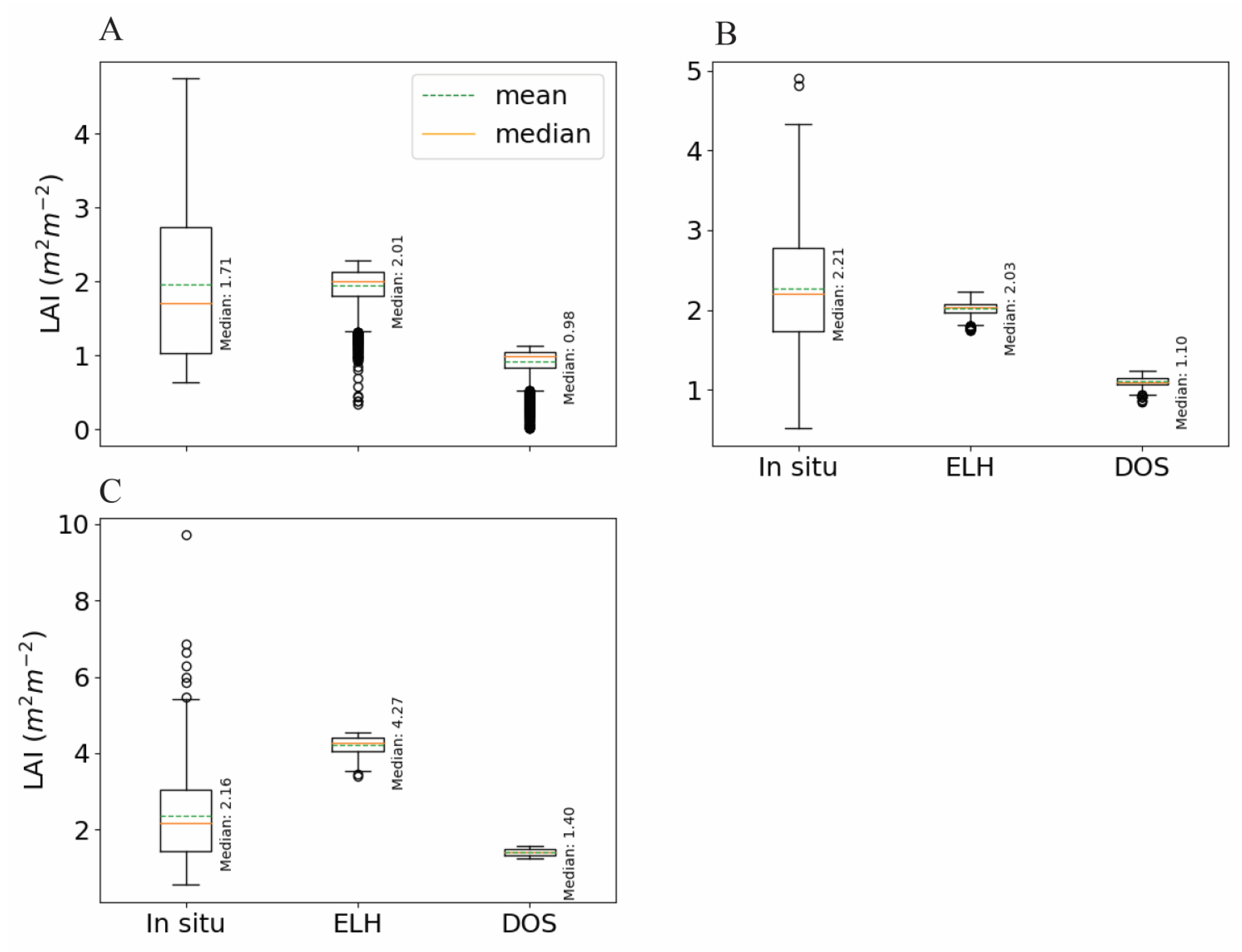
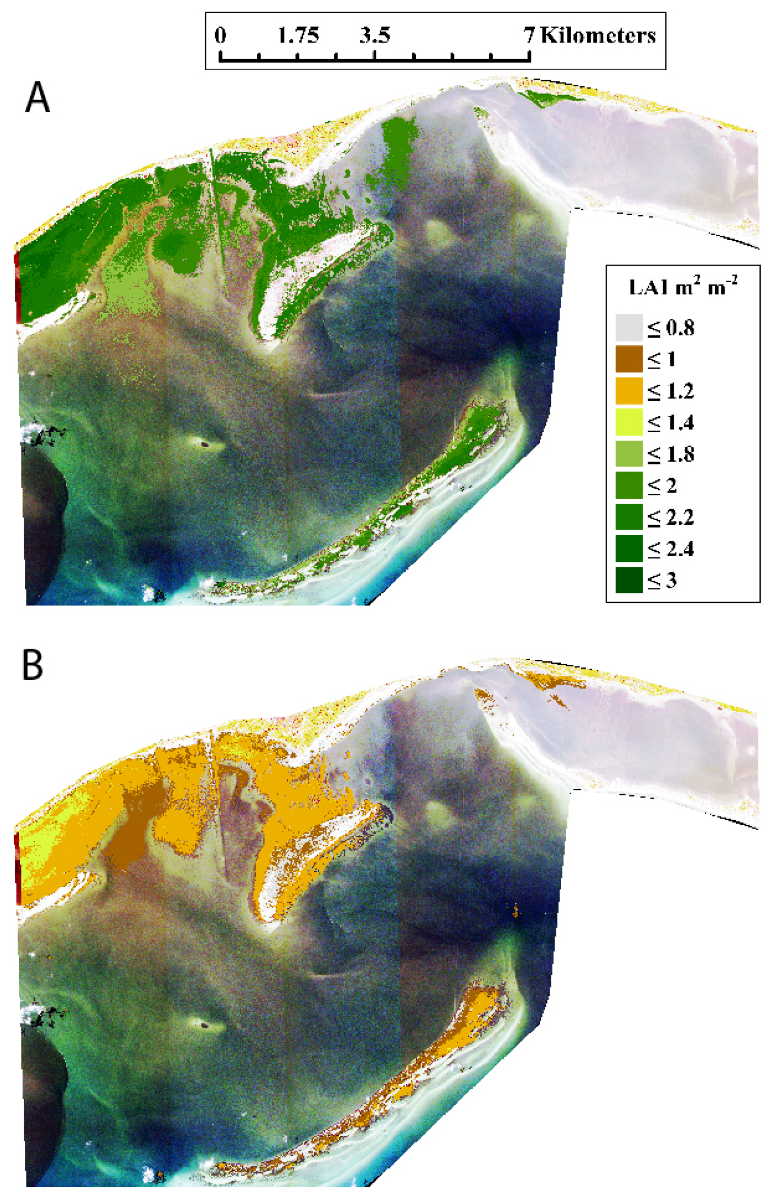
3.4.2. Saint Joseph Bay

LAI was spatially variable throughout Saint Joseph Bay (Figure 10A). The densest areas identified in the ELH image were in the shallow waters at the southern end of the bay, reaching 2.6 m² leaf m⁻² ground. The median LAI of the whole bay was 1.89 m² leaf m⁻² ground (

Table 7. Retrieved leaf area index (LAI) and derived above-ground carbon from Saint Joseph Bay, Saint George Sound, and Keaton Beach. Results are shown for LAI_(ELH) and LAI_(DOS). Statistics are calculated from all pixels classified as seagrass with LAI greater than 0 m² m⁻² in each raster.

	Saint Joseph Bay		Saint George Sound		Keaton Beach
Variable	LAI(ELH)	LAI(DOS)	LAI(ELH)	LAI(DOS)	LAI(ELH)	LAI(DOS)
Median LAI (m2 m−2)	1.97	0.98	1.96	1.06	3.33	1.41
Mean LAI (m2 m−2)	1.89	0.93	1.94	1.06	3.38	1.39
Min LAI	0	0	0	0	0	0
Max LAI	2.66	1.37	2.6	1.79	6.15	1.84
Total AGCseagrass (Gg)	1.66	0.88	1.24	0.62	8.34	3.53
Percent Differences from ELH		−47		−50		−58
Area-specific AGCseagrass (g m−2)	66	33	68	36	118	49

). The seagrass density decreased sharply as the deeper edges of the meadows transitioned to bare sand. AGC_seagrass in Saint Joseph Bay estimated from LAI_(ELH) was 1.66 Gg, with an area-specific carbon density of 66 g m⁻² (Table 7). Although the spatial pattern of seagrass distribution retrieved from R_rs(ELH) was similar to that produced using R_rs(DOS) (Figure 10A,B), LAI_(DOS) was approximately 50% lower than LAI_(ELH) across the entire image (median LAI 0.98 m² leaf m⁻² ground, Table 7 and Figure 10B). Correspondingly, the underestimation of LAI reduced the bay-wide AGC_seagrass by 47% to 0.88 Gg (Table 7). LAIs obtained through in situ measurements (LAI_{(IN SITU)}) were not significantly different from the retrieved LAI_(ELH) from pixels within our station locations (

Table 8. Results of pairwise Mann–Whitney tests to compare satellite-based LAI values with in situ observations for each study site. Raster values were collected from a 20 m radius around the in situ station locations (Figure 1). Symbol * indicates a significant difference.

	Saint Joseph Bay			Saint George Sound			Keaton Beach
	LAI(INS ITU)	LAI(ELH)	LAI(DOS)	LAI(INS ITU)	LAI(ELH)	LAI(DOS)	LAI(INS ITU)	LAI(ELH)	LAI(DOS)
LAI(INS ITU)		U = 280,464 p = 0.118	U = 423,261 p = <0.00 *		U = 126,423 p = 0.000 *	U = 285,869 p = <0.00 *		U = 36,241 p = <0.00 *	U = 377,731 p = <0.00 *
LAI(ELH)			U = 51,225,352 p = <0.00 *			U = 1,084,540 p = <0.00 *			U = 114,048 p = <0.00 *
LAI(DOS)

and Figure 11A). There were, however, notable differences in the range of values between these two datasets, with the LAI_{(IN SI)} exhibiting a substantially broader span in comparison to the values retrieved via satellite. The distribution of LAI_(ELH) values exclusively fell within the interquartile range of the in situ dataset but failed to capture LAI values surpassing 2.5 m² m⁻², densities that were observed in situ. LAI_(DOS) values were significantly lower than observed in situ (Table 8), with the majority of LAI_(DOS) values falling below the lower quartile of the LAI_{(IN SITU)} and entirely below the lowest LAI_(ELH) values (Figure 11A).

3.4.3. Saint George Sound

LAI_(ELH) values were high along the mainland shore of Saint George Sound behind the complex of shallow sandbars created by Lanark Reef and Turkey Point Reef and along the leeward edge of Dog Island Reef that separates the Sound from the Gulf of Mexico (Figure 12A). The median LAI_(ELH) across the scene was 1.96 m² leaf m⁻² seafloor, and the highest LAI_(ELH) of ~2.6 m² leaf m⁻² seafloor was found in the relatively turbid shallow water (~0.5 m deep) close to shore (Figure 12A). Similar densities (~2.6 m² leaf m⁻² ground) were found in the meadows occupying the deeper (~2 m) but clearer waters along the lee of Dog Island Reef. The total AGC_seagrass derived from LAI_(ELH) was 1.24 Gg, with an area-specific carbon of 68 g m⁻² (Table 7). As with Saint Joseph Bay, LAI_(DOS) values were ~50% lower than LAI_(ELH) (Figure 12B), reducing the estimation of total AGC_seagrass to 0.62 Gg and the area-specific carbon to 36g m⁻² (Table 7).

While the median values of LAI_{(IN SITU)} and LAI_(ELH) appear to be similar (Figure 11B), the two datasets were found to be significantly different (Table 8) due to the small dynamic range of LAI_(ELH). The middle 50% of LAI_(ELH) encompassed values of 1.98 to 2.10 m² leaf m⁻² ground (Figure 11B), in contrast to the larger range observed in LAI_{(IN SITU),} from 1.7 to 2.8 m² leaf m⁻² ground. With such a narrow range of distribution of LAI_(ELH), the higher and lower range of values measured in situ was not resolved. As in Saint Joseph Bay, both the mean and median of LAI_(DOS) fell below the lower quartile of the in situ dataset and entirely below the lowest LAI_(ELH) retrieval (Figure 11B), making these retrievals significantly different from both LAI_(ELH) and LAI_{(IN SITU)} (Table 8)_.

3.4.4. Keaton Beach

The seagrass at Keaton Beach occupied a 3 km wide band of homogeneous density ~3 m² leaf m⁻² ground parallel to the shore (Figure 13A). The 2 m isobath marked the edge of the continuous seagrass meadow, with densities dropping sharply to bare sand, transitioning to optically deep water. The median LAI_(ELH) was the highest of all three regions at 3.33 m² leaf m⁻² ground (Figure 13A and Table 7). Both the higher total area and densities in Keaton Beach were reflected in the highest AGC_seagrass and area-specific carbon of all three study sites at 8.34 Gg, with an area-specific carbon of 118 g m² (Table 7). As with the other two sites, LAI_(DOS) was lower than LAI_(ELH) (Figure 13B), which translated into a 58% underestimation of AGC_seagrass calculated from LAI_(DOS) compared to that from LAI_(ELH) (Table 7).

When comparing co-located LAI_{(IN SITU)} and LAI_(ELH), the satellite retrievals were found to be significantly higher (Table 8), exceeding the upper quartile of the in situ data while remaining within the range of the maximum values (Figure 11C). Although the mean LAI_(ELH) was greater, the retrievals effectively capture the elevated in situ densities observed at this site when compared to Saint Joseph Bay and Saint George Sound. LAI_(DOS) was significantly lower than LAI_{(IN SITU)} (Table 8), exhibited a significantly narrower range of values when compared to LAI_(ELH), and had the greatest divergence from LAI_(ELH) of all three sites (Figure 11C).

3.4.5. LAI_(ELH) Compared to LAI_(DOS)

The underestimation of LAI from R_rs(DOS) relative to both R_rs(ELH) was a consistent pattern across all three sites (Figure 14). The highly predictive relationship between LAI_(ELH) and LAI_(DOS) (r² 0.94) can be approximated across the entire dataset with an exponential function (Figure 14A and

Table 9. Regression parameters for data presented in Figure 13. Values in parentheses are standard errors of the slope and intercept.

Algorithm #	Fit Type	Site	Slope	Intercept	Exponent	r2
1	Exponential	All (Figure 14A)	0.39 (0.0044)	1.53 (0.0063)	4.289 (0.05)	0.96
2	Linear	Saint Joseph Bay (Figure 14B)	1.63 (0.004)	0.41 (0.006)		0.90
3	Linear	Saint George Sound (Figure 14C)	1.03 (0.017)	0.89 (0.017)		0.79
4	Exponential	Keaton Beach (Figure 14D)	0.171 (0.03)	2.12 (0.079)	5.59 (0.359)	0.85

). When analyzed separately, the relationships at both Saint Joseph Bay and Saint George Sound were best represented by linear functions (Figure 14B,C and Table 9), while the Keaton Beach fit remained slightly exponential (Figure 14D and Table 9).

Using either the single exponential function that encompassed all the sites or the individual linear/exponential models specific to each site, the accuracy of correcting LAI_(DOS) to values equivalent to LAI_(ELH) was high (

Table 10. Statistical output comparing accuracy of regression models for predicting LAI from LAI_(DOS) when using regression relationships detailed in Table 9.

Site	Algorithm	Mean Absolute Error	Root-Mean-Square Error
Saint Joseph Bay	1	0.089	0.11
	2	0.0419	0.068
Saint George Sound	1	0.114	0.148
	3	0.0422	0.061
Keaton Beach	1	0.084	0.185
	4	0.130	0.175

). Using algorithm 1, the mean absolute error (MAE) at all three sites was less than 0.2 m² leaf m⁻² ground, which is approximately 10% of the mean LAI values for Saint Joseph Bay and Saint George and 6% for Keaton Beach. The root-mean-square error (RMSE) was similar in magnitude to the MAE (Table 10), with the greatest errors occurring for LAI predicted at Saint George Sound. Using algorithms tuned for individual study sites improved both the MAE and RMSE for Saint Joseph Bay and Saint George Sound by approximately 50%, reducing the error in the predicted LAI to less than 5% of the mean values (Table 10). For Keaton Beach, an individual exponential fit increased MAE over algorithm 1 and produced only a small improvement in RMSE.

4. Discussion

This study revealed that the use of published radiometric calibration factors combined with DOS atmospheric correction produced images with much higher reflectances than those produced by empirical calibration of the raw satellite images against direct ground observations. However, the residual brightness, which we assume to be primarily atmospheric contamination but could include radiometric calibration inaccuracy, did not dramatically affect the supervised classification of seagrass presence in these optically complex coastal environments. Classification differences between the ELH and DOS methods were most apparent at the transition zones defining the shallow and deep edges of the meadows, but these transition zones represented a relatively small fraction of the total area. Thus, the choice of atmospheric correction method may not be critical for detecting the presence of seagrass beds, but it may be important for accurately identifying the boundaries of the meadows. Furthermore, the residual brightness in the green band resulting from the DOS approach caused the retrievals of seagrass LAI, and therefore, the carbon biomass, to be underestimated by approximately 50% compared to the ELH-processed image, which showed a stronger concordance with in situ measurements. Nonetheless, our comparison provides a potential path for rectifying DOS-based LAI retrievals that may permit seagrass LAI and above-ground carbon to be estimated from the existing collection of WorldView-2 images that lack in situ observations needed to accurately correct atmospheric interference in the green region of the spectrum.

Residual atmospheric contamination leading to higher radiances, especially in the blue and green bands, relative to in situ observations has been observed in both WorldView-2 and other high-spatial-resolution sensors, such as Pleiades, Sentinel-2, and Landsat-5 and 7 [30,33,34], and may be a widespread problem in atmospheric correction methods generally (B. Collister, NASA, pers comm). Coffer et al. [3] compared WorldView-2 R_rs after DOS correction to in situ observations and concluded that it may not be just an atmospheric correction problem, as uncalibrated drift in post-launch sensor responsivity may also play a role.

Despite the presence of high residual radiances in the blue and green bands (bands 1 and 2), the classification of the DOS-processed image successfully separated seagrass pixels from optically shallow sand and optically deep water in three distinct WorldView-2 images that represented a range of optically complex waters characteristic of coastal Florida. This indicates that the WorldView-2 archive can be used to produce reliable supervised classification maps of seagrass distributions, even when atmospheric correction is imperfect.

The differences in the seagrass area between ELH- and DOS-corrected images were found to account for less than 8% of the total coverage, primarily resulting from the overclassification of (i) optically shallow bare sand along the deep margins and (ii) intertidal environments vegetated by benthic algae as seagrass from R_rs(DOS). These misclassifications were caused not only by the overestimation of R_rs(DOS) but also by the narrow dynamic range seen in the blue band, which limits the ability to resolve targets with small spectral differences, such as the shallow edges of the seagrass meadows and green intertidal environments. The ELH method better replicated the true spectral shape of sea surface R_rs, preserving the larger dynamic range in all bands, but especially in the blue band, which improved the resolution of some boundaries between the deeper seagrass meadows and bare sand that were spectrally indistinguishable in the DOS image.

A few estimates of the seagrass area for these sites are available for comparison. In September 2006, airborne hyperspectral imagery was collected at Saint Joseph Bay, from which seagrass was estimated to cover 18.3 km² [23]. The flight lines did not cover the northernmost section of the bay, which may account for the slightly lower estimate. A 30-year analysis of seagrass populations in Saint Joseph Bay between 1990 and 2021 using Landsat 5 through 8 imagery returned areal estimates varying from 17.5 to 27 km², with no discernable temporal trend [5], placing our 2010 estimate at the higher end of seagrass coverage estimates. Variations in the total seagrass coverage in Saint Joseph Bay have been linked to hurricanes, which can cause short-term (6-month) declines in seagrass [5].

Importantly, our DCNN analysis of this multispectral imagery generated a classification map of Saint Joseph Bay that was nearly identical to that achieved with hyperspectral imagery collected over the same site in 2006 [23] that included an intertidal class dominated by filamentous red algae. However, Hill et al. (2014) also demonstrated how the delineation of the seagrass habitat deteriorated when the spatial resolution was coarsened beyond 10 m. Thus, the ability to generate similar classification results with multispectral and hyperspectral sensors suggests that the greatest need in categorical classification coastal remote sensing may be spatial rather than spectral resolution.

Seagrass Density Quantification

Although the ELH imagery produced seagrass densities that were comparable to in situ observations, direct comparisons to the latter present challenges due to the small-scale spatial heterogeneity found in seagrass meadows. This heterogeneity results in larger variances in shoot counts measured by small quadrats (e.g., 0.04 m²) within a 20 m radius than in corresponding satellite pixels at the same locations. At our sites, in situ seagrass densities exhibited high variability on small scales, ranging from sparse to dense within a few meters. This variability is reflected in the large range of LAI observed in the in situ datasets. In contrast, the coarser spatial resolution of the WorldView-2 sensor (4 to 9 m²) resulted in lower variability in retrieved LAI due to the integration of the bottom reflectance signal over the larger footprint of each pixel. Despite the limitations in assessing match-ups between remotely sensed and in situ seagrass densities, LAI_(ELH) in Saint Joseph Bay and Saint George Sound from pixels within our in situ station locations did show similarity to the mean densities measured in situ. At Keaton Beach, the mean LAI_(ELH) from our station locations was double the mean from the collocated in situ observations. However, high seagrass densities were prevalent in the in situ counts conducted at Keaton Beach, as seen in the presented box plots, which show a skew toward higher LAI, with several high-density quadrats more than 5 m² leaf m⁻² ground. LAI_(ELH) retrievals at Keaton Beach did resolve lower densities closer to the coastline, which is seen when considering the whole Keaton Beach image, which had a mean of 3.38 m² leaf m⁻² ground.

At all sites, the imagery effectively captured density variations across the underwater landscape, which can provide crucial insights into the spatial ecology of seagrass meadows. The ability to differentiate between sparse and dense seagrass can be critical in the management of seagrass resources, as sparse areas are more susceptible to disturbances, and therefore, the retrieval of density from satellites provides a tool to aid in the early detection of changes.

The underestimation of LAI_(DOS) was caused by the residual reflectance in band MS3 (green) remaining after calibration/atmospheric correction. The strong correlation between LAI_(DOS) and LAI_(ELH) provides a mechanism for correcting LAI_(DOS) to values equivalent to those retrieved from an image with accurate atmospheric correction (i.e., ELH). Both the comprehensive regression encompassing all datasets and the individual regressions for each dataset yielded high accuracy in correcting LAI_(DOS). This study therefore indicates that there exists a model to correct the underestimation of LAI_(DOS) that is stable across a 2-year gap and 220 km of the Gulf of Mexico coastline, which supports a considerable range of water column optical properties.

LAI_(DOS) was also underestimated in a study utilizing Landsat 5 images of Saint Joseph Bay [5]. The offset in that case was a simple upward correction of LAI_(DOS) of 0.98, indicating that while the underestimation of LAI from incomplete atmospheric correction is prevalent, the LAI correction may be sensor-specific.

WorldView-2 was tasked to collect the images used in this study, but an archive of images extending back to 2010 is available over other coastal areas with seagrass. Although it appears that the use of published radiometric calibration values and DOS atmospheric correction are sufficient for the reliable classification of areal distribution, the retrieval of biogeochemically relevant products such as LAI and, therefore, AGC_seagras) may be underestimated without in situ measurements to apply accurate calibration/atmospheric correction. Ultimately, the robustness of this correction needs to be further studied if it is to be a pathway for processing the WorldView-2 archive for density and Blue Carbon estimates. Further studies of LAI retrieved from WorldView-2 using available atmospheric correction methods will be needed to determine whether underestimation is consistent across geographical regions and sensors.

5. Conclusions

WorldView-2 provides sufficient spectral resolution to separate spectral characteristics of seagrass from the surrounding benthic targets in optically complex waters. Accuracy in atmospheric correction was found to be less important than precision in enabling the identification of seagrass. Therefore, images could be classified routinely even if atmospheric contaminants remain in the data. Incomplete atmospheric correction appears to be universal in the blue and green regions of the spectrum and not just in WorldView-2 images; therefore, we expect that without accounting for this omission, the seagrass density will be consistently underestimated from coastal imagery. As coincident in situ R_rs measurements are not available with most image collections, the development and testing of an empirical correction to LAI is a critical step for carbon retrieval from WorldView-2 and other sensors.

WorldView-2 and other high-spatial-resolution satellites provide the ability to retrieve the absolute density on a per-pixel basis, as opposed to classifying polygons using relatively broad categories of percent cover. The benefit of retrieving LAI lies in the strong correlation between the density and above-ground seagrass carbon, which in turn can be used to estimate below-ground carbon. The percent seagrass cover is a commonly retrieved attribute that can be estimated via manual delineation of aerial imagery or through sea surface reflectance, but unlike LAI, it is not strongly predictive of biomass [19]. For this reason, we suggest that finding an appropriate correction for LAI when residual brightness remains in the spectra after atmospheric correction or finding a way to improve our atmospheric correction is critical in moving our estimates forward for the seagrass contribution to Blue Carbon.

References

1. Chmura, G.; Short, F.; Torio, D.; Arroyo-Mora, P.; Fajardo, P.; Hatvany, M.; van Ardenne, L. North America’s Blue Carbon: Assessing Seagrass, Salt Marsh and Mangrove Distribution and Carbon Sinks: Project Report; Commission for Environmental Cooperation: Montreal, Canada, 2016; p. 54. [Google Scholar]
2. McKenzie, L.J.; Nordlund, L.M.; Jones, B.L.; Cullen-Unsworth, L.C.; Roelfsema, C.; Unsworth, R.K. The global distribution of seagrass meadows. Environ. Res. Lett. 2020, 15, 074041. [Google Scholar] [CrossRef]
3. Coffer, M.; Schaeffer, B.A.; Zimmerman, R.C.; Hill, V.; Li, J.; Islam, K.A.; Whitman, P.J. Performance across WorldView-2 and RapidEye for reproducible seagrass mapping. Remote Sens. Environ. 2020, 250, 112036. [Google Scholar] [CrossRef] [PubMed]
4. Koedsin, W.; Intararuang, W.; Ritchie, R.J.; Huete, A. An Integrated Field and Remote Sensing Method for Mapping Seagrass Species, Cover, and Biomass in Southern Thailand. Remote Sens. 2016, 8, 292. [Google Scholar] [CrossRef]
5. Lebrasse, M.C.; Schaeffer, B.A.; Coffer, M.; Whitman, P.J.; Zimmerman, R.C.; Hill, V.J.; Islam, K.A.; Li, J.; Osburn, C.L. Temporal Stability of Seagrass Extent, Leaf Area, and Carbon Storage in St. Joseph Bay, Florida: A Semi-automated Remote Sensing Analysis. Estuaries Coasts 2022, 45, 2082–2101. [Google Scholar] [CrossRef] [PubMed]
6. Misbari, S.; Hashim, M. Change Detection of Submerged Seagrass Biomass in Shallow Coastal Water. Remote Sens. 2016, 8, 200. [Google Scholar] [CrossRef]
7. Phinn, S.; Roelfsema, C.; Dekker, A.; Brando, V.; Anstee, J. Mapping seagrass species, cover and biomass in shallow waters: An assessment of satellite multi-spectral and airborne hyper-spectral imaging systems in Moreton Bay (Australia). Remote Sens. Environ. 2008, 112, 3413–3425. [Google Scholar] [CrossRef]
8. Pu, R.; Bell, S. Mapping seagrass coverage and spatial patterns with high spatial resolution IKONOS imagery. Int. J. Appl. Earth Obs. 2017, 54, 145–158. [Google Scholar] [CrossRef]
9. Roelfsema, C.M.; Lyons, M.; Kovacs, E.M.; Maxwell, P.; Saunders, M.I.; Samper-Villarreal, J.; Phinn, S.R. Multi-temporal mapping of seagrass cover, species and biomass: A semi-automated object based image analysis approach. Remote Sens. Environ. 2014, 150, 172–187. [Google Scholar] [CrossRef]
10. Wicaksono, P.; Maishella, A.; Arjasakusuma, S.; Lazuardi, W.; Harahap, S.D. Assessment of WorldView-2 images for aboveground seagrass carbon stock mapping in patchy and continuous seagrass meadows. Int. J. Remote Sens. 2022, 43, 2915–2941. [Google Scholar] [CrossRef]
11. Zoffoli, M.L.; Gernez, P.; Rosa, P.; Le Bris, A.; Brando, V.E.; Barillé, A.-L.; Harin, N.; Peters, S.; Poser, K.; Spaias, L. Sentinel-2 remote sensing of Zostera noltei-dominated intertidal seagrass meadows. Remote Sens. Environ. 2020, 251, 112020. [Google Scholar] [CrossRef]
12. Veettil, B.K.; Ward, R.D.; Lima, M.D.A.C.; Stankovic, M.; Hoai, P.N.; Quang, N.X. Opportunities for seagrass research derived from remote sensing: A review of current methods. Ecol. Indic. 2020, 117, 106560. [Google Scholar] [CrossRef]
13. National Research Council. Climate Data Records from Environmental Satellites: Interim Report; National Academies Press: Washinton, DC, USA, 2004. [Google Scholar]
14. Kaufman, K.A.; Bell, S.S. The Use of Imagery and GIS Techniques to Evaluate and Compare Seagrass Dynamics across Multiple Spatial and Temporal Scales. Estuaries Coasts 2020, 45, 1028–1044. [Google Scholar] [CrossRef]
15. Meehan, A.; Williams, R.; Watford, F. Detecting trends in seagrass abundance using aerial photograph interpretation: Problems arising with the evolution of mapping methods. Estuaries 2005, 28, 462–472. [Google Scholar] [CrossRef]
16. Bell, S.S.; Fonseca, M.S.; Stafford, N.B. Seagrass ecology: New contributions from a landscape perspective. In Seagrasses: Biology, Ecology and Conservation; Springer: Berlin/Heidelberg, Germany, 2007; pp. 625–645. [Google Scholar]
17. Islam, K.A.; Hill, V.; Schaeffer, B.A.; Zimmerman, R.C.; Li, J. Semi-supervised Adversarial Domain Adaptation for Seagrass Detection Using Multispectral Images in Coastal Areas. Data Sci. Eng. 2020, 5, 111–125. [Google Scholar] [CrossRef]
18. Islam, K.A.; Pérez, D.; Hill, V.; Schaeffer, B.A.; Zimmerman, R.C.; Li, J. Seagrass detection in coastal water through deep capsule networks. In Proceedings of the Chinese Conference on Pattern Recognition and Computer Vision (PRCV); Springer: Cham, Switzerland, 2018; pp. 320–331. [Google Scholar]
19. Simpson, J.; Bruce, E.; Davies, K.P.; Barber, P. A Blueprint for the Estimation of Seagrass Carbon Stock Using Remote Sensing-Enabled Proxies. Remote Sens. 2022, 14, 3572. [Google Scholar] [CrossRef]
20. Costanza, R.; d’Arge, R.; De Groot, R.; Farber, S.; Grasso, M.; Hannon, B.; Limburg, K.; Naeem, S.; O’neill, R.V.; Paruelo, J. The value of the world’s ecosystem services and natural capital. Nature 1997, 387, 253–260. [Google Scholar] [CrossRef]
21. Jänes, H.; Carnell, P.; Young, M.; Ierodiaconou, D.; Jenkins, G.P.; Hamer, P.; Zu Ermgassen, P.S.; Gair, J.R.; Macreadie, P.I. Seagrass valuation from fish abundance, biomass and recreational catch. Ecol. Indic. 2021, 130, 108097. [Google Scholar] [CrossRef]
22. Dierssen, H.M.; Zimmerman, R.C.; Leathers, R.A.; Downes, T.V.; Davis, C.O. Ocean color remote sensing of seagrass and bathymetry in the Bahamas Banks by high-resolution airborne imagery. Limnol. Oceanogr. 2003, 48, 444–455. [Google Scholar] [CrossRef]
23. Hill, V.J.; Zimmerman, R.C.; Bissett, P.; Dierssen, H.M.; Kohler, D. Evaluating Light Availability, Seagrass Biomass, and Productivity Using Hyperspectral Airborne Remote Sensing in Saint Joseph’s Bay, Florida. Estuaries Coasts 2014, 37, 1467–1489. [Google Scholar] [CrossRef]
24. Hemminga, M.A.; Duarte, C.M. Seagrass Ecology Seagrass; Cambridge University Press: Cambridge, UK, 2000. [Google Scholar]
25. Van Tussenbroek, B.I. Above- and below-ground biomass and production by Thalassia tesudinum in a tropical reef. Aquat. Bot. 1998, 61, 69–82. [Google Scholar] [CrossRef]
26. Sfriso, A.; Ghetti, P.F. Seasonal variation in biomass, morphometric parameters and production of seagrasses in the lagoon of Venice. Aquat. Bot. 1998, 61, 207–223. [Google Scholar] [CrossRef]
27. cKarpouzli, E.; Malthus, T. The empirical line method for the atmospheric correction of IKONOS imagery. Int. J. Remote Sens. 2003, 24, 1143–1150. [Google Scholar] [CrossRef]
28. Collin, A.; Hench, J.L. Towards Deeper Measurements of Tropical Reefscape Structure Using the WorldView-2 Spaceborne Sensor. Remote Sens. 2012, 4, 1425–1447. [Google Scholar] [CrossRef]
29. Wicasksono, P.; Hafizt, M. Dark target effectiveness for dark-object subtraction atmospheric correction method on mangrove above-ground carbon stock mapping. IET Image Process. 2018, 12, 582. [Google Scholar] [CrossRef]
30. Eugenio, F.; Marcello, J.; Martin, J.; Rodríguez-Esparragón, D. Benthic habitat mapping using multispectral high-resolution imagery: Evaluation of shallow water atmospheric correction techniques. Sensors 2017, 17, 2639. [Google Scholar] [CrossRef] [PubMed]
31. Agapiou, A.; Hadjimitsis, D.G.; Papoutsa, C.; Alexakis, D.D.; Papadavid, G. The importance of accounting for atmospheric effects in the application of NDVI and interpretation of satellite imagery supporting archaeological research: The case studies of Palaepaphos and Nea Paphos sites in Cyprus. Remote Sens. 2011, 3, 2605–2629. [Google Scholar] [CrossRef]
32. De Keukelaere, L.; Sterckx, S.; Adriaensen, S.; Knaeps, E.; Reusen, I.; Giardino, C.; Bresciani, M.; Hunter, P.; Neil, C.; Van der Zande, D. Atmospheric correction of Landsat-8/OLI and Sentinel-2/MSI data using iCOR algorithm: Validation for coastal and inland waters. Eur. J. Remote Sens. 2018, 51, 525–542. [Google Scholar] [CrossRef]
33. Vanhellemont, Q.; Ruddick, K. Atmospheric correction of metre-scale optical satellite data for inland and coastal water applications. Remote Sens. Environ. 2018, 216, 586–597. [Google Scholar] [CrossRef]
34. Vanhellemont, Q. Adaptation of the dark spectrum fitting atmospheric correction for aquatic applications of the Landsat and Sentinel-2 archives. Remote Sens. Environ. 2019, 225, 175–192. [Google Scholar] [CrossRef]
35. Stewart, R.A.; Gorsline, D.S. Recent Sedimentary History of St. Joseph Bay, Florida St. Joseph Bay. Sedimentology 1962, 1, 256–286. [Google Scholar] [CrossRef]
36. Big Bend Seagrasses Aquatic Preserve. Big Bend Seagrasses Aquatic Preserve Management Plan; Big Bend Seagrasses Aquatic Preserve: Crystal River, FL, USA, 2015. [Google Scholar]
37. Cannizzaro, J.P.; Carlson, P.R., Jr.; Yarbro, L.A.; Hu, C. Optical variability along a river plume gradient: Implications for management and remote sensing. Estuar. Coast. Shelf Sci. 2013, 131, 149–161. [Google Scholar] [CrossRef]
38. Pegau, W.S.; Zaneveld, R.V.; Mueller, J.L. Volume Absorption Coefficients: Instruments, Characterization, Field Measurements and Data Analysis Protocols. In Ocean Optics Protocols for Satellite Ocean Color Sensor Validation; Mueller, J.L., Fargion, G.S., McClain, C.R., Eds.; NASA: Greenbelt, MD, USA, 2003; Revision 4; Volume 4. [Google Scholar]
39. Pope, R.; Fry, M.E.S. Absorption spectrum (380–700 nm) of pure water. Part II: Integrating cavity measurements. Appl. Opt. 1997, 36, 8710–8723. [Google Scholar] [CrossRef] [PubMed]
40. Mobley, C.D. Light and Water: Radiative Transfer in Natural Waters; Academic Press: San Diego, CA, USA, 1994. [Google Scholar]
41. Morel, A.; Mueller, J.L. Normalized Water-Leaving Radiance and Remote Sensing Reflectance: Bidirectional Refelctance and Other Factors; Goddard Space Flight Center: Greenbelt, MD, USA, 2003; pp. 32–59.
42. Zimmerman, R.C.; Hill, V.; Bissett, P.; Mobley, C.D. Empirical Line Fits. In The Ocean Optics Book; Mobley, C.D., Ed.; International Ocean Colour Coordinating Group (IOCCG): Dartmouth, NS, Canada, 2022; pp. 590–594. [Google Scholar]
43. Mobley, C.D. A Numerical-Model for the Computation of Radiance Distributions in Natural-Waters with Wind-Roughened Surfaces. Limnol. Oceanogr. 1989, 34, 1473–1483. [Google Scholar] [CrossRef]
44. Chavez, P.S. An improved dark-object subtraction technique for atmospheric scattering correction of multispectral data. Remote Sens. Environ. 1988, 24, 459–479. [Google Scholar] [CrossRef]
45. Kuester, M. Absolute Radiometric Calibration. 2017. Available online: https://dg-cms-uploads-production.s3.amazonaws.com/uploads/document/file/209/ABSRADCAL_FLEET_2016v0_Rel20170606.pdf (accessed on 31 July 2023).
46. Schaeffer, B.A.; Myer, M.H. Resolvable estuaries for satellite derived water quality within the continental United States. Remote Sens. Lett. 2020, 11, 535–544. [Google Scholar] [CrossRef]
47. McFeeters, S.K. The use of the Normalized Difference Water Index (NDWI) in the delineation of open water features. Int. J. Remote Sens. 1996, 17, 1425–1432. [Google Scholar] [CrossRef]
48. Bishop, C.M. Pattern Recognition and Machine Learning; Springer: Berlin/Heidelberg, Germany, 2006; Available online: https://catalogue.library.cern/literature/yqnn7-y0x04 (accessed on 31 July 2023).
49. CIRES. Cooperative Institute for Research in Environmental Sciences (CIRES) at the University of Colorado, B. Continuously Updated Digital Elevation Model (CUDEM)—1/9 Arc-Second Resolution Bathymetric-Topographic Tiles; CIRES: Boulder, CO, USA, 2014. [Google Scholar] [CrossRef]
50. Kruskal, W.H.; Wallis, W.A. Use of ranks in one-criterion variance analysis. J. Am. Stat. Assoc. 1952, 47, 583–621. [Google Scholar] [CrossRef]
51. Mann, H.B.; Whitney, D.R. On a test of whether one of two random variables is stochastically larger than the other. Ann. Math. Stat. 1947, 18, 50–60. [Google Scholar] [CrossRef]
52. Virtanen, P.; Gommers, R.; Oliphant, T.E.; Haberland, M.; Reddy, T.; Cournapeau, D.; Burovski, E.; Peterson, P.; Weckesser, W.; Bright, J. SciPy 1.0: Fundamental algorithms for scientific computing in Python. Nat. Methods 2020, 17, 261–272. [Google Scholar] [CrossRef]
53. Duarte, C.M. Seagrass depth limits. Aquat. Bot. 1991, 40, 363–377. [Google Scholar] [CrossRef]
54. Batiuk, R.; Bergstrom, P.; Kemp, W.M.; Koch, E.W.; Murry, L.; Stevenson, J.; Bartleson, R.; Carter, V.; Rybicki, N.; Landwehr, J.; et al. Chesapeake Bay Submerged Aquatic Vegetation Water Quality and Habitat-Based Requirements and Restoration Targets: A Second Synthesis; Chesapeake Bay Program Office: Annapolis, MD, USA, 2000. [Google Scholar]
Figure 1. Mercator projection showing the three study regions located along the Florida Gulf Coast, USA, and the three WorldView-2 images analyzed in this study. From left to right, Saint Joseph Bay, Saint George Sound, and Keaton Beach. Underlying imagery sources: CONANP, Esri, Garmin, FAO, NOAA, USGS, EPA, Earthstar Geographics.
Remotesensing 15 04715 g001
Figure 2. RGB images of all three study sites, stretched using histogram equalization (γ = 0.5) to assist visualization of spectral differences. (A). St. Joseph Bay. (B). St. George Sound. (C). Keaton Beach. Mapped are the locations of stations used for atmospheric correction (white) and those that were fully characterized with respect to water column optics and seagrass abundance (purple) and Regions of Interest (ROIs) used for DCNN classification.
Remotesensing 15 04715 g002
Figure 3. Flowchart of image-processing steps.
Remotesensing 15 04715 g003
Figure 4. Mean spectra for (A) absorption (apg), (B) scattering (bp), and (C) beam attenuation (cpg) coefficients measured using Sea-Bird/WetLabs ac-9 instrument in Saint Joseph Bay, Saint George Sound, and Keaton Beach. Error bars indicate ±1 standard error of the mean for each wavelength bin.
Remotesensing 15 04715 g004
Figure 5. Comparison between Rrs retrieval for ELH and DOS atmospheric correction for WV-2 bands MS2 through MS7. Data for each site are indicated by symbol color. Dotted line represents the 1:1 line of perfect agreement. Data consist of 300 randomly chosen points from each site, 100 from seagrass, 100 from submerged sand, and 100 from deep water.
Remotesensing 15 04715 g005
Figure 6. Habitat classification maps for Saint Joseph Bay using (A) ELH atmospheric correction and (B) DOS atmospheric correction. Habitat class is indicated by color identified in the legend in (A). (C) Comparison of pixels identified as seagrass using ELH and DOS atmospheric correction. Pixels mapped in green were identified by both. Pixels mapped in blue and red were identified only by DOS and ELH, respectively.
Remotesensing 15 04715 g006
Figure 7. Habitat classification maps for Saint George Sound using (A) ELH atmospheric correction and (B) DOS atmospheric correction. (C) Comparison of pixels identified as seagrass using ELH and DOS atmospheric correction. Pixels mapped in green were identified by both. Pixels mapped in blue and red were identified only by DOS and ELH, respectively. The rectangular and circular shapes highlight areas that are mentioned in the text.
Remotesensing 15 04715 g007
Figure 8. Habitat classification maps for Keaton Beach using (A) ELH atmospheric correction and (B) DOS atmospheric correction. Habitat class is indicated by color identified in the legend in Figure 6A. (C) Comparison of pixels identified as seagrass using ELH and DOS atmospheric correction. Pixels mapped in green were identified by both. Pixels mapped in blue and red were identified only by DOS and ELH, respectively.
Remotesensing 15 04715 g008
Figure 9. In situ measurements of Rb(green) and leaf area index from all three study sites. LAI values are averaged from randomized sampling within 20 m of a central location and are shown with ±1 standard error bars.
Remotesensing 15 04715 g009
Figure 10. Maps of leaf area index (LAI) retrieval for Saint Joseph Bay calculated from (A) Rrs(ELH) and (B) Rrs(DOS).
Remotesensing 15 04715 g010
Figure 11. Box-and-whisker plots for LAI measured in situ and retrieved from LAI(ELH) and LAI(DOS) from pixels collected from a 20 m radius around the in situ station locations (Figure 1). (A). Saint Joseph Bay, (B). Saint George Sound, (C). Keaton Beach.
Remotesensing 15 04715 g011
Figure 12. Maps of leaf area index (LAI) retrieved for Saint George Sound calculated from (A) Rrs(ELH) and (B) Rrs(DOS).
Remotesensing 15 04715 g012
Figure 13. Maps of leaf area index (LAI) retrieval for Keaton Beach calculated from (A) Rrs(ELH) and (B) Rrs(DOS).
Remotesensing 15 04715 g013
Figure 14. LAI(DOS) versus LAI(ELH) from 1000 randomly selected pixels from each site. (A). All sites combined. (B). Saint Joseph Bay. (C). Saint George Sound. (D). Keaton Beach Dotted line represents the 1:1 line, and points above this line are higher in the LAI(ELH) retrieval.
Remotesensing 15 04715 g014