
Age Identification of Farmland Shelterbelt Using Growth Pattern Based on Landsat Time Series Images
1
Northeast Institute of Geography and Agroecology, Chinese Academy of Sciences, Changchun 130102, China
2
University of Chinese Academy of Sciences, Beijing 100049, China
3
Jilin Provincial Academy of Forestry Sciences, Changchun 130033, China
4
College of Surveying and Geo-Informatics, North China University of Water Resources and Electric Power, Zhengzhou 450046, China
*
Author to whom correspondence should be addressed.
Remote Sens. 2023, 15(19), 4750; https://doi.org/10.3390/rs15194750
Submission received: 24 July 2023
/
Revised: 1 September 2023
/
Accepted: 25 September 2023
/
Published: 28 September 2023
Abstract
:Farmland shelterbelt, as a category of shelterbelt in forestry ecological engineering, has an important influence on agricultural sustainability in agricultural systems. Timely and accurate acquisition of farmland shelterbelt age is not only essential to understanding their shelter effects but also directly relates to the adjustment of subsequent shelterbelt projects. In this study, we developed an age identification method using growth pattern to extract the age of shelterbelt (i.e., years after planting) based on Landsat time series images. This method was applied to a typical area of shelterbelt construction in the north of Changchun, China. The results indicated that the accuracy of age identification reached a stable situation when the permissible age error exceeded 3 years, achieving an accuracy of approximately 90%. Moreover, the accuracy at different growth phases (1–3 years, 4–15 years, 16–30 years, and >30 years) decreased with increasing age, and the accuracy of each growth phase can reach more than 80% when the permissible age error is beyond 7 years. Compared to building the typically weak statistical relationship between the shelterbelt age and remote sensing characteristic information to derive age, this method presented a direct age identification method for fine-scale age extraction of the shelterbelt. It introduced a novel perspective for shelterbelt age identification and the assessment of shelterbelt project advancement on the regional scale.
1. Introduction
As an important part of the agroforestry ecosystem, farmland shelterbelt not only has vital ecological effects in reducing wind speed and changing the microclimate environment of cropland but also brings important ecological benefits in reducing soil nutrient loss, maintaining wildlife habitat, and stabilizing food production [1,2,3,4,5]. Farmland shelterbelt lacks the ability of independent renewal. As a type of artificial forest, it must be renewed by manual intervention to ensure the sustainability of the shelterbelt project.
Age serves as a critical parameter for characterizing the growth status of farmland shelterbelt, directly influencing the process of shelterbelt renewal. The timely and precise identification of shelterbelt age is imperative for the sustainable management of shelterbelt and for evaluating the progress of shelterbelt project construction [6].
The traditional method of obtaining shelterbelt age primarily involves field investigation based on tree ring analysis [7]. Age determination can also be achieved indirectly by utilizing statistical relationships between other structural parameters of the shelterbelt and its age [8,9,10]. However, employing the aforementioned method is challenging to implement on a large scale due to the labor-intensive and time-consuming nature of data collection. Currently, remote sensing technology has been proven to be a powerful tool for forests monitoring and age acquisition on a large scale [11,12,13,14,15].
Given that remote sensing images cannot directly ascertain the age of the forest, it becomes imperative to establish a connection between remote sensing data and age information [14,16,17]. Many researchers employed the spectral index characteristics of single-scene optical images, SAR, or LiDAR scattering data to establish correlations between feature variables and age. Age determination through this method is a classic approach and has been validated in various research. Jensen, et al. [18] used one-scene Landsat TM satellite images to extract spectral and vegetation index information as input parameters for an artificial neural network (ANN) to identify the age of coniferous forests in southern Brazil and concluded that there was a high correlation between age and vegetation index. Trisasongko [13] implemented the extraction of rubber tree age using single SAR images by extracting polarization and spatial texture features using machine learning algorithms such as random forest (RF) and support vector machine (SVM), respectively, and revealed a high correlation between the age of rubber trees and the texture and dual polarization features of ALOS-2. When relying on single-scene images to determine forest ages, the distinctions in characteristic variables among forest images of similar ages tend to be minimal. These images are substantially influenced by temporal phases and environmental conditions, rendering it challenging to discern age-related changes precisely.
To address this disadvantage, multi-temporal remote sensing can more precisely capture surface information from dynamic changes [19,20,21,22]. Time series analysis relying on multi-temporal images can acquire the evolving characteristics of forest growth across both temporal and spatial dimensions. As a result, this approach offers a viable method for determining the age of shelterbelt. Li and Fox [23] imported a total of 29 MODIS NDVI data from 2009 to 2010 to the Mahalanobis distance classifier, successfully overcoming the problem of age overestimation at the early stage of rubber growth, and extracted both young (<4 years old) and mature (>=4 years old) rubber trees. Fujiki, et al. [24] combined a high-resolution satellite image (WorldView-2) with Landsat time series images and extracted ages from a change-detection analysis. After using regression models and decision tree discriminant analysis for rubber of different ages (1–3 years, 3–5 years, 5–7 years, 7–30 years, 30–50 years, >50 years, and ‘rubber plantations’), the validation showed that the age accuracy of rubber was 84.3%. Chen et al. [25] used Landsat annual time series and developed a robust integrated pixel and object-based tree growth model that successfully produced a rubber forest age map with 30 m resolution, with an accuracy of 87.00% for identifying rubber plantation. Obtaining forest age based on multi-temporal remote sensing images has achieved reliable results, but previous studies have focused on patchy natural or artificial forests. For farmland shelterbelt, which exhibits the characteristics of belt-shaped artificial forests, it is crucial to conduct additional research aimed at accurately extracting ages based on their growth characteristics. Deng et al. [26] divided the farmland shelterbelt into three growth stages, used time series Landsat data to estimate the age of the farmland shelterbelt over a two-year monitoring period, and made an initial attempt at remote-sensing-based farmland shelterbelt age estimation.
The main objective of this study is to develop an automatic age extraction method with universal applicability to improve the identification accuracy of the farmland shelterbelt age. The workflow of this study is as follows: (1) first, we extracted fractional coverage characteristic values of each shelterbelt annually, generating fractional coverage of a farmland shelterbelt (FCFS) curve from 1984 to 2021; (2) after preprocessing the abnormal values of each FCFS curve, the shelterbelt was divided into three growth patterns according to the FCFS curve combined with the characteristics of the shelterbelt projects and the algorithm was designed to identify the age of shelterbelt; (3) finally, a typical construction area of the shelterbelt was selected to validate the age identification method, and the age distribution of the shelterbelt in this area was evaluated.
2. Materials
2.1. Study Area
The study area is located in the north of Changchun (central at 44°31′35.0″N, 125°27′50″E, Figure 1), which is situated on the Songnen Plain. It includes parts of Dehui City, Nong’an County, and Jiutai District, with a total area of 3600 km2. This area is in the distribution zone of black soil in Northeast China, which is the key construction area of the Three North (3N) Shelterbelt Project, with a long history of farmland shelterbelt planting. Due to severe wind damage in spring, as early as before the implementation of the 3N Shelterbelt Project, small-scale farmland shelterbelt has been planted in this region, forming the unique agroforestry landscape with the staggered distribution of shelterbelt and cropland, which played an indispensable role in resisting wind damage [27,28,29]. Since the implementation of the 3N Shelterbelt Project in 1978, after nearly 50 years of construction, this region has basically formed a complete distribution system of shelterbelt.
2.2. Landsat Time Series Data Pre-Processing
Landsat time series data were acquired from the US Geological Survey (http://earthexplorer.usgs.gov/ (accessed on 15 November 2022)). The data’s product level was L1TP, indicating they had undergone corrections for topography and radiation. The temporal coverage spanned from 1984 to 2021. One scene (path/row: 118/029) could cover the study area. During the selected time period (days 120–180 of the year), farmland shelterbelt exhibits significant differences from cropland. An optimal image for each year was selected based on the criteria of cloud cover being less than 50%, combined with visual interpretation. Finally, a total of 32 images were chosen for the purpose of age identification. The remote sensing data sources and the time distribution of image acquisition in different years were shown in Figure 2. Due to a large amount of cloud, there were no available images in 1990, 1993, 1995, 2000, 2010, and 2012. In addition, it should be noted that more than a third of the selected 32 images were affected to varying degrees by clouds, which was the main factor that affected the accuracy of growth patterns division and age identification, and the solutions will be deliberated in Section 3.2.2.
Affected by different sensors and image-acquired date, it was particularly necessary for radiometric calibration correction for the obtained images each year. By reading metadata-file-stored spectral band gain and offset numbers that can be used to linearly convert the digital numbers to at-sensor radiance (Wm−2 sr−1μm−1) and to convert the digital numbers to sensor reflectance, we completed radiometric calibration [30,31]. The atmospheric corrections were conducted by FLAASH correction algorithm to convert Atmospheric Top Reflectance to Surface Reflectance Product [32,33]. After completing the above preprocessing for each image, the normalized difference vegetation index (NDVI) [34] was calculated annually, and the study area was clipped.
2.3. Shelterbelt Construction Status Data
The construction status data of shelterbelt were obtained by artificial visual interpretation. Based on Landsat 8 OLI image on 31 May 2021, Google Earth Pro was used as a reference for interpretation. The shelterbelt was represented as line elements and interrupted at the intersection points, and the shelterbelt was drawn as integrity when the break occurs. Only the shelterbelt of more than 100 m was retained for subsequent age identification. Through field research and validation, the accuracy of interpreting shelterbelts could exceed 90%.
2.4. Validation Data
2.4.1. Fractional Coverage of Shelterbelt Data
The fractional coverage of shelterbelt (FCFS) is an important parameter reflecting the growth status of farmland shelterbelt. The true FCFS data were captured using the DJI Magic 2 Pro camera in a vertical downward orientation, capturing 5–10 photos per sample point. In order to compare with the fractional coverage of Landsat image inversion, the acquisition time was close to the Landsat image time (collection in 2019, 2020, 2021). A comprehensive selection of 15 shelterbelts, encompassing 78 sample points, was conducted, considering a range of ages and growth conditions.
First, each image was cropped to fit each of the targeted stand extents. Second, after cropping the targeted range, the Excess green index (ExG) was calculated by using the following formula (Equation (1)) to highlight the canopy information of the shelterbelt [35,36,37]:
where G, R, and B are values in green, red, and blue contents. Through manual threshold adjustment, the imagery underwent a process of binarization, segregating it into two categories: shelterbelt and non-shelterbelt canopy. Finally, the proportion of the area occupied by the shelterbelt canopy was calculated, and the FCFS data of each sample point were acquired by calculating an average of the FCFS value from the multiple photos obtained.
ExG = 2G − R − B
2.4.2. Shelterbelt Age Data
All age data used in this paper to validate the accuracy of shelterbelt age identification algorithm were obtained in three ways: (1) visually interpreted based on Landsat time series images combined with Google Earth Pro history images; (2) on-site interviewed with shelterbelt growers; (3) the tree core of the annual growth cone was collected and analyzed by professionals. Considering the actual status of the study area, the age data of 357 shelterbelts were collected by random sampling, ranging from 2 years to more than 35 years.
3. Methods
3.1. Dimidiate Pixel Model Inversion Fractional Coverage
The farmland shelterbelt is mostly distributed around the cropland. Considering the characteristics of the staggered distribution of shelterbelt and cropland, it fits well with the prerequisites of the dimidiate pixel model [38,39]. Therefore, the dimidiate pixel model was chosen to calculate fractional coverage in this study [40,41,42]; this study used NDVI to calculate the fractional coverage (FC):
where NDVImixed is the mixed pixel, NDVIcropland is the NDVI value of cropland endmember, and NDVIveg is the NDVI value of vegetation endmember. It is very important for inversion results to accurately obtain the NDVIcropland and NDVIveg values when applying dimidiate pixel model to calculate fractional coverage. In order to reduce the abnormal change in inter-annual fractional coverage caused by the selection of endmember and ensure the comparability, the following rules were used to select endmember in this paper:
FC = (NDVImixed − NDVIcropland)/(NDVIveg − NDVIcropland)
- (1)
- The endmember sample points of vegetation and cropland were selected by visual interpretation on Landsat time series images combined with existing Google Earth Pro historical images and field observation.
- (2)
- The sample points were evenly distributed where cropland did not change from 1984 to 2021. The NDVI of cropland was extracted annually and the mean value was calculated as the endmember value of cropland (NDVIcropland) in each image.
- (3)
- The sample points were evenly distributed in the image of densely distributed (>5 × 5 pixels) patch poplar forests. Since the patchy forest will change over time, the spatial distribution of the sample points was adjusted according to the inter-annual variation, and the NDVI of vegetation was extracted annually and the mean value was calculated as the vegetation endmember value (NDVIveg) of each image.
Finally, the obtained endmember values of vegetation and cropland from 1984 to 2021 were used to calculate fractional coverage.
3.2. Build FCFS Curve of Time Series
3.2.1. Extract FCFS Value
The fractional coverage data from 1984 to 2021 and the construction status data (2021) of the shelterbelt were superimposed and extracted using a waveform collector [43], which was perpendicular to the direction of the shelterbelt in 3 × 3 neighborhood window to acquire the maximum waveform sequence of each shelterbelt in each year. The maximum waveform sequence of FCFS value reflects the integrity of shelterbelt structure. Figure 3 shows the maximum waveform changes of the selected typical shelterbelt (integrity and missing).
To obtain the FCFS value that reflects the characteristics of shelterbelt, it is necessary to filter and extract the valid values from the FCFS maximum waveform sequence. This process should take into account the integrity of the shelterbelt. In our research, we used the standard deviation (SD) of the maximum waveform sequence as a reference to judge the structural integrity of the shelterbelt and filter the valid values. According to the comparative analysis of the SD of the selected typical integrity and the missing shelterbelt, 0.05 was chosen as the threshold for judgment. The calculation method of the FCFS value representing the characteristics of shelterbelt is
- (1)
- When the SD < 0.05, the shelterbelt structure is regarded as integrity, and all the FCFS values in the maximum waveform sequence are regarded as valid values; m is the total number of pixel sequences of the FCFS.
- (2)
- When the SD >= 0.05, the shelterbelt structure is incomplete (missing). The valid values are the FCFS value greater than the mean value of the maximum waveform sequence, and n is the id number of valid pixel sequences greater than its mean value.
FCFSi = (FCFSi1984, FCFSi1985, …, FCFSij)
3.2.2. Time Series FCFS Curve Smooth
Among the collection of Landsat images utilized for building the time series FCFS curve, a noteworthy observation was that the years 1990, 1993, 1995, 2000, 2010, and 2012 lacked accessible images within the specified time range. Despite the availability of Landsat images in certain years, the FCFS values did not accurately represent reality due to the interference of clouds and other environmental factors (shadows, crop growth stages, and lush vegetation) near the shelterbelt. These were principal factors that affect the growth pattern division of shelterbelt, which were related to the accuracy of age identification. Therefore, it was necessary to smooth the missing and abnormal FCFS values and restore the real FCFS curve as much as possible. To reduce the influence of some factors on the time series of FCFS curve and not weaken the shelterbelt renewed information, we divided the influence into positive and negative effects:
- (1)
- The positive effect is reflected in the enhancement of the FCFS value, which is mainly reflected in the dense vegetation (forests or grass) near the shelterbelt, so that the FCFS value is significantly higher than that of the nearby years (FCFSij > FCFSij-1 AND FCFSij > FCFSij+1), and this part will form a significant peak value in the time series FCFS curve.
- (2)
- The negative effect is reflected in the weakening of the FCFS value, mainly due to the cover of the cloud (shadows or image missing), which leads to the FCFS value being significantly lower than that of the nearby years (FCFSij < FCFSij-1 AND FCFSij < FCFSij+1). This issue also presents a significant challenge in age identification, resulting in the formation of pronounced valley values within the time series FCFS curve.
To not weaken the renewed year information of the shelterbelt as much as possible, we need to judge whether the FCFS value of the year (FCFSij) is at the peak or valley value annually. If a peak or valley exists, a subsequent assessment is conducted to determine whether FCFSij is a normal fluctuation. If the fluctuation range is less than the threshold Z (|FCFSij+1 − FCFSij-1| < Z; Z is the normal growth fluctuation interval of FCFS value at one year), Equation (5) is then executed:
FCFSij = (FCFSij − 1 + FCFSij + 1)/2
If the fluctuation range is equal to or larger than the threshold Z, the smoothing operation is not performed. Based on the analysis of FCFS alterations in shelterbelts at one-year intervals (Figure 4), it is evident that approximately 50% of the shelterbelts exhibit changes ranging from 0.03 to 0.11. Considering the inherent growth patterns of the shelterbelt, a change in FCFS interval of 0.1 within a year is deemed reasonable (Z = 0.1). Until the smoothing process has been completed for all shelterbelts for each year of FCFS values and no peak (valley) value meets the conditions, the smoothing is stopped.
3.3. Growth Pattern Division and Age Identification
3.3.1. Determination Initial Recognition Characteristics of Remote Sensing
Because of the influence of Landsat’s spatial resolution, the newly planted shelterbelt may not be immediately visible in Landsat images after renewal. Generally, they become distinguishable on Landsat images around 2–4 years after planting. To derive the FCFS value of initial recognition on the Landsat, we selected the fractional coverage value of the farmland shelterbelt (2–4 years) and the factional coverage value of the cropland (Figure 5) by field sampling combined with remote sensing retrieval. During the initial growth of the shelterbelt (2–4 years), the factional coverage change range remains narrow, with approximately 50% of the shelterbelt exhibiting changes within the range of 0.1 to 0.18. Notably, this range differs substantially from that observed in cropland (0.02–0.07). We chose 0.15 as the judgment threshold for the initial recognition of shelterbelt. It was considered that the shelterbelt could be recognized on the Landsat images when the FCFS value was higher than 0.15, and the shelterbelt cannot be recognized when it was lower than that threshold.
Figure 6a reflects the growth process of the selected typical shelterbelt from 2013 to 2021 (chopped in 2014; planted new shelterbelt in 2015) on Landsat images. The Landsat satellite images showed that the new shelterbelt was displayed on the images for 2 to 4 years after renewal. The FCFS curve of this typical shelterbelt after renewal is shown in Figure 6b. When the threshold was set to 0.15, the initial recognition age of the shelterbelt on the Landsat image was over 3 years after planting (2018). To divide the growth pattern and age identification of shelterbelt, this paper uniformly considered the shelterbelt can be initially recognized on the Landsat after 3 years of planting. Considering the number of different planting rows, we randomly selected some typical shelterbelts for validation. The results indicated that selecting 3 years as the initial recognition age in Landsat images was in line with reality.
3.3.2. Growth Pattern Analysis
After long-term monitoring of shelterbelt combined with the curves of FCFS based on the Landsat time series, we divided the shelterbelt into three growth patterns and generated the simulated FCFS curve (Figure 7):
- (1)
- Pattern one: The shelterbelt existed in the early stage of monitoring, and continuous planting was not interrupted. Renewing occurred during the monitoring time, and the times of renewal were less than two. Figure 7a shows the simulated curve of FCFS for this growth pattern. When the renewal occurs, the FCFS value decreased abruptly and remained at a low value for a continuous period. Based on the existing recorded data, the majority of shelterbelts had experienced only one-time renewal, which was reflected in an abrupt change in the FCFS value. When occurring multiple renewals, there were multiple pronounced abrupt points.
- (2)
- Pattern two: No shelterbelt was planted in the initial stage. After the planning of the shelterbelt project, shelterbelt was planted. Figure 7b is the simulation FCFS curve of this growth pattern. They showed that FCFS value was always at a low value when no shelterbelt was planted in the early stage of growth, and the shelterbelt was gradually recognized in the Landsat over 2–4 years of planting. If an FCFS value equal to 0.15 was used as the threshold for the presence or absence of shelterbelt, the FCFS value was below this threshold until the shelterbelt was planted and recognized.
- (3)
- Pattern three: The shelterbelt existed at the beginning of the monitoring period and did not undergo renewal. When the shelterbelt belonged to this pattern, the value of FCFS was always high; except for the influence of external factors such as cloud and shadow, the overall FCFS value was higher than 0.15 (Figure 7c). The shelterbelt of such growth patterns was all more than 30 years old, focusing on this shelterbelt that needs to be renewed orderly.
3.3.3. Age Identification Based on Growth Pattern
According to the three growth patterns of shelterbelt based on the FCFS curve of Landsat time series in Section 3.3.2, we set up the following rules to discriminate the growth pattern of shelterbelt and identified the age according to the characteristics of growth patterns. When the shelterbelt belonged to pattern one, the FCFS value in the year of chopping will have a large difference from the previous years, showing a steep drop. By calculating the first-order difference (Equations (6) and (7)), the threshold value can be set to locate the year with the first-order difference anomaly [24,44].
FCFSi = (FCFSi1984, FCFSi1985, …, FCFSi2021)
Diff-FCFSi = (Diff-FCFSi1985, Diff-FCFSi1986, …, Diff-FCFSi2021)
Based on a statistical analysis of the FCFS curve, the change value of inter-annual FCFS (Diff-FCFSij) was less than or equal to 0.1; we thought it was within a reasonable growth variation interval. When it was greater than that threshold (anomaly), we thought there were two cases as follows: (1) shelterbelt chopping; (2) data anomalies caused by missing data and interference from external factors. We set that the year of the differential anomaly was j and H was the initial recognition year of the shelterbelt that can be identified in the Landsat time series (j < H <= 2021). If there existed H, it satisfies Equation (8):
FCFSiH >= 0.15 AND FCFSiH-1 < 0.15 AND FCFSiH-2 < 0.15 AND FCFSiH-3 < 0.15
Then, the year of planting was H-3, and the age of the shelterbelt was 2021-(H-3) years. If there were more eligible Hs (multiple renewals occurred), we chose the maximum of H as the initial recognition year, and, if there were no j and H that met this condition, the shelterbelt was classified as growth pattern two or three.
When the shelterbelt belonged to growth pattern two or three, it could not meet our premise assumption of growth pattern one because the shelterbelt had not experienced renewal. Therefore, we took the observation year (2021) as the benchmark and judged year by year whether the FCFS value was below the threshold (0.15 was taken in this paper, and the FCFS value below 0.15 was regarded as unrecognition in Landsat). When there existed H (1987 =< H <= 2021) satisfying the condition of Equation (8), the shelterbelt belonged to growth pattern two and the year of planting was H-3, and the age of the shelterbelt was 2021-(H-3) years. If there was no H that met the condition, the shelterbelt belonged to growth pattern three, and the age was regarded as more than 33 years.
3.4. Accuracy Assessment
The correlation coefficient (R2) and root mean square error (RMSE) and the mean absolute error (MAE) were used to evaluate the correlation between the FCFS obtained from the dimidiate pixel model and the truth FCFS. Moreover, we used the accuracy (Equation (9)) to assess the accuracy of farmland shelterbelt age identification method using the Landsat time series.
where n is the number of shelterbelts whose ages are correctly extracted, and N is the total number of shelterbelts used for validation. To further validate the performance of the age extraction method proposed in different age phases, we also used the confusion matrix to evaluate the age identification results. This evaluation encompassed metrics such as overall accuracy, commission, and omission.
Accuracy = n/N × 100%
4. Results
4.1. Remote Sensing Inversion of FCFS
The FCFS based on Landsat images is very important for the growth pattern and age identification of shelterbelts. Therefore, it is necessary to evaluate the results of the dimidiate pixel model retrieval. The FCFS derived through dimidiate pixel inversion exhibited a strong correlation with the truth FCFS (coefficient of determination R2 = 0.766, p < 0.01, Figure 8). Additionally, the mean absolute error (MAE) and root mean square error (RMSE) were calculated as 0.1093 and 0.1332, respectively. The inversion results revealed that the dimidiate pixel inversion presented a viable alternative for acquiring FCFS. This approach can subsequently be employed for time series processing and the division of shelterbelt growth patterns.
4.2. Evaluation of Shelterbelt Age Identification Accuracy
Based on the research on the management of shelterbelt [45,46,47], combined with the age identification method in our research, we divided the age of shelterbelt into the following four phases: early planting (1–3 years); pre-protection maturity (4–15 years); protection maturity (16–30 years); and renewal (more than 30 years).
We selected a total of 357 shelterbelts for validation of the accuracy of the age identification algorithm based on growth patterns. Figure 9a showed the trend in the accuracy change with the permissible error age (permissible error age = |truth age-identification age|). When the permissible error was 0 years, the accuracy was only about 54%; as the permissible error was beyond 15 years, the accuracy reached 95%. The accuracy rapidly increased with the permissible error until 3 years and then slowly rose and gradually stabilized at approximately 90%.
Figure 9b indicated the trend in the accuracy of the shelterbelt at different age phases with increasing permissible error. The overall trend was that, with the increase in age, the accuracy of the shelterbelt age extracted by the method proposed in this paper tended to decrease, among which the accuracy of early planting (1–3 years) was the highest (95%); it basically did not change with the change in the permissible error. When the permissible error was 0 years, the accuracy of renewal (more than 30 years) was the lowest and only 19%. Moreover, when the permissible error was less than 7 years, the accuracy rate can reach more than 80% regardless of age phases. As depicted in Figure 9b, it is obvious that, when the permissible error was below 7 years, the accuracy of renewal (more than 30 years) was the lowest. However, when the permissible error surpassed 7 years, a significant increase in accuracy was observed, bringing it closer to the accuracy of the early planting phase (1–3 years).
To further evaluate the extraction accuracy of the method proposed in this study on the age of shelterbelt at different ages phases, we used the overall accuracy, commission, and omission in the confusion matrix to evaluate the precision of the age-extracted results (Table 1).
Table 1 divided the ages into four different growth phases with an overall accuracy of 85.15%. In terms of commission, the average commission was 0.1658, with a high commission of 0.3191 between 16 and 30 years. Shelterbelts aged 16–30 years were particularly susceptible to being misclassified as belonging to the more than 30 years category. The lowest commission was observed in the age of 4–15 years, with a value of 0.0443. The average omission was calculated to be 0.1670, with a significantly higher omission observed for the age phase of more than 30 years, reaching a value of 0.3617. The lowest omission was 1–3 years (0.0166). The results of the commission and omission showed that 16–30 years and more than 30 years were the most likely to misclassify, and the accuracy of the extracted age was slightly lower compared to the other age phases. In summary, the method proposed in this paper to identify the age of shelterbelt based on growth patterns exhibited satisfactory accuracy.
4.3. Age Mapping Analysis in the Study Area
Using the age identification method based on the growth pattern of shelterbelt proposed, a spatial distribution map of the shelterbelt age and statistical diagram of the growth pattern in the study area (2021) were acquired. Figure 10 showed that the shelterbelt spatial distribution of all ages in the study area was even, and there was no obvious spatial aggregation of the same age.
According to the statistics of the age of shelterbelt in the study area (Figure 11a), the shelterbelt of 4–15 years and 16–30 years in the region accounted for the highest proportion, the total accounting for more than 70%. The shelterbelt of these two age phases was also the main shelterbelt that influences the shelter effects. In addition, 20.9% of the shelterbelts were more than 30 years old, while only 8.5% fell within 1–3 years of age. From the statistics of the growth patterns of the shelterbelt in the study area (Figure 11b), the highest percentage of growth pattern one (42.4%) was slightly higher than that of growth pattern two (37.2%), which indicated that the renewed and newly planned shelterbelts were the main types of shelterbelts in this study area. As for growth pattern three, although it was far lower than the other growth patterns, it still occupied a considerable proportion (20.4%).
Figure 11c showed the composition of different growth patterns. In the 1–3 years of shelterbelts, growth pattern two accounted for 65%, while growth pattern one only accounted for 35%, indicating that the number of newly planned shelterbelts in these phases was much higher than the renewed. In the shelterbelts of 4–15 years, growth pattern one accounted for 58%, while growth pattern two accounted for 42%, and the shelterbelts of renewed were slightly higher than the newly planned in this age phase. Growth patterns one (45%) and two (55%) in the 16–30 years shelterbelts were not significantly different, and the new planned shelterbelts were slightly higher than the renewed shelterbelts. Among shelterbelts with an age of over 30 years old, the vast majority (99.6%) corresponded to growth pattern three, whereas only a minimal proportion fell within growth pattern two.
5. Discussion
5.1. Analysis of Age Error Sources
Through an analysis of shelterbelts with inaccurately extracted ages, it was observed that the primary factors influencing the accuracy of this method include:
- (1)
- Missing remote sensing image and continuous interference from clouds and others. Because of the limitations of the sensors and weather conditions, when shelterbelt images were missed at key time nodes of growth (renewal or initial planting) years or had been affected by clouds or other external influences for several consecutive years, it would cause anomalies in the local FCFS curve. Even if the smoothing method proposed in this paper was used, it was difficult to restore the FCFS curve truly, leading to the incorrect division of the shelterbelt growth pattern, which in turn will result in wrong age identification.
- (2)
- Accuracy of the dimidiate pixel model when applied to the medium resolution remote images (30 m, Landsat) inversion fractional coverage of farmland shelterbelt. The spatial resolution of Landsat series satellite image is 30 m, and the canopy width of farmland shelterbelt is generally between 10 and 30 m, so the images of the shelterbelt are all mixed pixels. Due to the influence of the stand environment, the changes between the shelterbelt and the cropland at the pixel level may not always conform to the linear changes, causing interference to the subsequent FCFS curve.
- (3)
- The characteristics value setting of remote sensing data in the judgment of the growth pattern of shelterbelt. When setting the threshold for the initial recognition of farmland shelterbelt on Landsat, we selected 3 years after planting that could be recognized on the image based on the characteristics of the shelterbelt. Meanwhile, we set the FCFS value greater than 0.15 as the threshold for initial recognition on Landsat. However, due to the influence of the number of rows planted, the spacing between rows, and the time of the available Landsat images, there were fluctuations in the year of initial identification characteristics. Therefore, the uniform setting of a fixed threshold will inevitably lead to misjudgment, affecting the shelterbelt age identification.
In this study, a methodology was devised to identify the age of farmland shelterbelt based on the growth pattern. The results showed good identification accuracy (Figure 9), but the accuracy was different for different age phases. When the shelterbelt age was more than 30 years, the identification accuracy was the lowest. However, when the permissible error was greater than 7 years, the accuracy of this age phase was improved, and it was gradually higher than other age phases (Figure 9b). According to the analysis of the data, the main reasons may be divided into the following: (1) the growth pattern of more than 30 years of shelterbelt was single, and, when it was misclassified, it was mainly misclassified as less than 30 years, and it is unlikely to be misclassified into other age phases (Table 1); (2) the earlier Landsat image quality was subpar (1984–1990), leading to inadequate representation of farmland shelterbelt information and subsequently resulting in potential misclassification of age (5–10 years). In addition, for shelterbelts between the age of 16 and 30 years, it was also easy to identify errors, particularly in being mistaken for those aged more than 30 years. It is imperative to enhance the age identification method to address this specific source of error.
The time of Landsat images used to build the time series FCFS curve in our research was from early May to late June [48]. However, the available remote sensing images had difficulty meeting the need for more accurate age identification in some years due to the weather conditions and the revisit cycle of Landsat satellites. To mitigate error sources, enhancing the quality of remote sensing data can prove effective in improving accuracy. When the crop harvesting period is at the end of September and the middle of October, notable spectral differences emerge in the spectrum of farmland shelterbelts [49]. Addressing the impact of temporal phases and leveraging it to estimate shelterbelt age requires in-depth investigation. In addition to utilizing Landsat series satellites, further research is needed to explore the integration of multi-source remote sensing satellite data (e.g., Sentinel-1, Sentinel-2, and SPOT) for estimating the age of farmland shelterbelt [50,51,52,53].
Regarding the age identification algorithm in our research, the threshold configuration within the proposed algorithm was determined by statistical analysis. Nonetheless, this approach did not account for the potential influence of shelterbelt tree species and other planting parameters, such as row count and spacing [54]. This limitation unavoidably led to a slight reduction in the accuracy of age identification. There is a requirement to improve both the process of setting thresholds and the criteria used for model evaluation, enhancing the precision of age identification.
5.2. Methods Comparison
Remote sensing technology holds substantial potential for the inversion of forest structure parameters and age extraction, yielding many research results [23,25,55,56]. Currently, remote sensing to acquire the forest age can be divided based on single-phase and multi-temporal images. Compared with relying on single-phase images for forest age determination, the utilization of multi-temporal images offers a richer source of forest growth information. This enables a more accurate extraction of forest age through a comprehensive consideration of its growth characteristics. In previous studies, the employment of multi-temporal images for forest age determination predominantly relied on statistical analysis methods, which constitute an indirect approach to age extraction. While these methods can yield remarkable results, challenges persist in terms of their widespread adoption [23,24,25,57].
Ideally, if the initial planting year of the shelterbelt can be obtained through time series analysis, it would enable the determination of the shelterbelt’s age [19,22,58]. In contrast to Zheng, et al. [59] only used a few phases of remote sensing images to obtain the age of the shelterbelt by visual interpretation; the method proposed in our research can automatically extract the age of shelterbelt, which can greatly reduce the workload. Based on the growth characteristics of farmland shelterbelts, Deng, et al. [26] categorized them into three different growth stages. A two-year monitoring period was employed to construct time-series growth state curves, enabling the identification age of the shelterbelt. In our research, the age was identified by determining the initial planting year based on the growth pattern of different farmland shelterbelts, considering the construction characteristics of shelterbelt as artificial forests. On the other hand, our method to identify the age of shelterbelt without setting too many parameters reduced the age identification errors caused by the definition of different parameters. In terms of age extraction accuracy, the accuracy of this method proposed in our study is 69% compared with Deng et al. [26] when the permissible error is within 1 year. We further discuss the accuracy changes of this method and the age identification accuracy of different age phases. The results show that our method is more robust for the farmland shelterbelt age identification.
6. Conclusions
We categorized farmland shelterbelt into three distinct growth patterns. The ages of farmland shelterbelt corresponding to these different growth patterns were determined by employing Landsat time series images. It had been observed that the age identification method attained a stable accuracy level of 90% when the permissible error was beyond 3 years, which could be competent for the needs of shelterbelt-stage-oriented management. The information acquired on the growth pattern of the shelterbelt could also provide a reference for evaluating the construction progress of the shelterbelt project. Enhancing the accuracy of age for shelterbelts across various age stages (e.g., 16–30 years or >30 years) remains an important area for further improvement. In future research, a critical focus should be on accurately extracting age information from time-series images based on characteristics of shelterbelt.
Author Contributions
X.Z.: Data processed, Wrote original draft. J.L., Review and edited. Y.L.: Methodology, Review and edited. R.D.: Analyzed the remote sensing data. G.Y.: Supervision. J.T.: Supervision. All authors have read and agreed to the published version of the manuscript.
Funding
This research was supported by the National Natural Science Foundation of China (31971723).
Data Availability Statement
The data presented in this study are available on request from the corresponding author.
Acknowledgments
We appreciate anonymous reviewers for their constructive comments, which help improve the quality of this manuscript.
Conflicts of Interest
The authors declare that they have no known competing financial interests or personal relationships that could have appeared to influence the work reported in this paper.
References
- Zhang, H.; Brandle, J.; Meyer, G.; Hodges, L. The relationship between open windspeed and windspeed reduction in shelter. Agrofor. Syst. 1995, 32, 297–311. [Google Scholar] [CrossRef]
- Cleugh, H.; Miller, J.; Böhm, M. Direct mechanical effects of wind on crops. Agrofor. Syst. 1998, 41, 85–112. [Google Scholar] [CrossRef]
- Jiao-jun, Z.; Feng-qi, J.; Takeshi, M. Spacing interval between principal tree windbreaks. J. For. Res. 2002, 13, 83–90. [Google Scholar] [CrossRef]
- Torita, H.; Satou, H. Relationship between shelterbelt structure and mean wind reduction. Agric. For. Meteorol. 2007, 145, 186–194. [Google Scholar] [CrossRef]
- Fang, H.; Aitkenhead, M. Quantifying farmland shelterbelt impacts on catchment soil erosion and sediment yield for the black soil region, northeastern China. Soil Use Manag. 2020, 37, 181–195. [Google Scholar] [CrossRef]
- Smith, M.M.; Bentrup, G.; Kellerman, T.; MacFarland, K.; Straight, R.; Ameyaw, L. Windbreaks in the United States: A systematic review of producer-reported benefits, challenges, management activities and drivers of adoption. Agric. Syst. 2021, 187, 103032. [Google Scholar] [CrossRef]
- Sun, J.; Hamel, J.F.; Gianasi, B.L.; Mercier, A. Correction to: ‘Age determination in echinoderms: First evidence of annual growth rings in holothuroids’ 2022 by Sun et al. Proc. Biol. Sci. 2022, 289, 20221872. [Google Scholar] [CrossRef]
- Ali, A. Forest stand structure and functioning: Current knowledge and future challenges. Ecol. Indic. 2019, 98, 665–677. [Google Scholar] [CrossRef]
- Parker, G.G. Tamm review: Leaf Area Index (LAI) is both a determinant and a consequence of important processes in vegetation canopies. For. Ecol. Manag. 2020, 477, 118496. [Google Scholar] [CrossRef]
- Nascimbene, J.; Marini, L.; Motta, R.; Nimis, P.L. Influence of tree age, tree size and crown structure on lichen communities in mature Alpine spruce forests. Biodivers. Conserv. 2008, 18, 1509–1522. [Google Scholar] [CrossRef]
- Chemura, A.; van Duren, I.; van Leeuwen, L.M. Determination of the age of oil palm from crown projection area detected from WorldView-2 multispectral remote sensing data: The case of Ejisu-Juaben district, Ghana. ISPRS J. Photogramm. Remote Sens. 2015, 100, 118–127. [Google Scholar] [CrossRef]
- Chen, B.; Cao, J.; Wang, J.; Wu, Z.; Tao, Z.; Chen, J.; Yang, C.; Xie, G. Estimation of rubber stand age in typhoon and chilling injury afflicted area with Landsat TM data: A case study in Hainan Island, China. For. Ecol. Manag. 2012, 274, 222–230. [Google Scholar] [CrossRef]
- Trisasongko, B.H. Mapping stand age of rubber plantation using ALOS-2 polarimetric SAR data. Eur. J. Remote Sens. 2017, 50, 64–76. [Google Scholar] [CrossRef]
- Racine, E.B.; Coops, N.C.; St-Onge, B.; Bégin, J. Estimating Forest Stand Age from LiDAR-Derived Predictors and Nearest Neighbor Imputation. For. Sci. 2014, 60, 128–136. [Google Scholar] [CrossRef]
- Kacic, P.; Kuenzer, C. Forest Biodiversity Monitoring Based on Remotely Sensed Spectral Diversity—A Review. Remote Sens. 2022, 14, 5363. [Google Scholar] [CrossRef]
- Dye, M.; Mutanga, O.; Ismail, R. Combining spectral and textural remote sensing variables using random forests: Predicting the age of Pinus patula forests in KwaZulu-Natal, South Africa. J. Spat. Sci. 2012, 57, 193–211. [Google Scholar] [CrossRef]
- Cohen, W.B.; Spies, T.A.; Fiorella, M. Estimating the age and structure of forests in a multi-ownership landscape of western Oregon, U.S.A. Int. J. Remote Sens. 1995, 16, 721–746. [Google Scholar] [CrossRef]
- Jensen, J.R.; Qiu, F.; Ji, M.H. Predictive modelling of coniferous forest age using statistical and artificial neural network approaches applied to remote sensor data. Int. J. Remote Sens. 1999, 20, 2805–2822. [Google Scholar]
- Kennedy, R.E.; Yang, Z.; Cohen, W.B. Detecting trends in forest disturbance and recovery using yearly Landsat time series: 1. LandTrendr—Temporal segmentation algorithms. Remote Sens. Environ. 2010, 114, 2897–2910. [Google Scholar] [CrossRef]
- Huang, C.; Goward, S.N.; Masek, J.G.; Gao, F.; Vermote, E.F.; Thomas, N.; Schleeweis, K.; Kennedy, R.E.; Zhu, Z.; Eidenshink, J.C.; et al. Development of time series stacks of Landsat images for reconstructing forest disturbance history. Int. J. Digit. Earth 2009, 2, 195–218. [Google Scholar] [CrossRef]
- Broich, M.; Hansen, M.C.; Potapov, P.; Adusei, B.; Lindquist, E.; Stehman, S.V. Time-series analysis of multi-resolution optical imagery for quantifying forest cover loss in Sumatra and Kalimantan, Indonesia. Int. J. Appl. Earth Obs. Geoinf. 2011, 13, 277–291. [Google Scholar] [CrossRef]
- Shen, Z.; Wang, Y.; Su, H.; He, Y.; Li, S. A bi-directional strategy to detect land use function change using time-series Landsat imagery on Google Earth Engine: A case study of Huangshui River Basin in China. Sci. Remote Sens. 2022, 5, 100039. [Google Scholar] [CrossRef]
- Li, Z.; Fox, J.M. Mapping rubber tree growth in mainland Southeast Asia using time-series MODIS 250 m NDVI and statistical data. Appl. Geogr. 2012, 32, 420–432. [Google Scholar] [CrossRef]
- Fujiki, S.; Okada, K.-I.; Nishio, S.; Kitayama, K. Estimation of the stand ages of tropical secondary forests after shifting cultivation based on the combination of WorldView-2 and time-series Landsat images. ISPRS J. Photogramm. Remote Sens. 2016, 119, 280–293. [Google Scholar] [CrossRef]
- Chen, G.; Thill, J.-C.; Anantsuksomsri, S.; Tontisirin, N.; Tao, R. Stand age estimation of rubber (Hevea brasiliensis) plantations using an integrated pixel- and object-based tree growth model and annual Landsat time series. ISPRS J. Photogramm. Remote Sens. 2018, 144, 94–104. [Google Scholar] [CrossRef]
- Deng, R.; Xu, Z.; Li, Y.; Zhang, X.; Li, C.; Zhang, L. Farmland Shelterbelt Age Mapping Using Landsat Time Series Images. Remote Sens. 2022, 14, 1457. [Google Scholar] [CrossRef]
- Hanjie, W. A simulation study on the eco-environmental effects of 3N Shelterbelt in North China. Glob. Planet. Chang. 2003, 37, 231–246. [Google Scholar] [CrossRef]
- Zeng, H.; Peltola, H.; Väisänen, H.; Kellomäki, S. The effects of fragmentation on the susceptibility of a boreal forest ecosystem to wind damage. For. Ecol. Manag. 2009, 257, 1165–1173. [Google Scholar] [CrossRef]
- Wang, H.; Takle, E.S. Model-simulated influences of shelterbelt shape on wind-sheltering efficiency. J. Appl. Meteorol. Climatol. 1997, 36, 695–704. [Google Scholar] [CrossRef]
- Song, C.; Woodcock, C.E.; Seto, K.C.; PaxLenney, M.; Macomber, S.A. Classification and Change Detection Using Landsat TM Data: When and How to Correct Atmospheric Effects? Remote Sens. Environ. 2001, 75, 230–244. [Google Scholar] [CrossRef]
- Roy, D.P.; Wulder, M.A.; Loveland, T.R.; Woodcock, C.E.; Allen, R.G.; Anderson, M.C.; Helder, D.; Irons, J.R.; Johnson, D.M.; Kennedy, R.; et al. Landsat-8: Science and product vision for terrestrial global change research. Remote Sens. Environ. 2014, 145, 154–172. [Google Scholar] [CrossRef]
- Schäfer, K.; Perkins, T.; Comerón, A.; Adler-Golden, S.; Matthew, M.; Slusser, J.R.; Picard, R.H.; Berk, A.; Anderson, G.; Carleer, M.R.; et al. Retrieval of atmospheric properties from hyper and multispectral imagery with the FLAASH atmospheric correction algorithm. In Remote Sensing of Clouds and the Atmosphere X; SPIE: Bellingham, WA, USA, 2005. [Google Scholar]
- Shen, S.S.; Felde, G.W.; Lewis, P.E.; Anderson, G.P.; Gardner, J.A.; Adler-Golden, S.M.; Matthew, M.W.; Berk, A. Water vapor retrieval using the FLAASH atmospheric correction algorithm. In Algorithms and Technologies for Multispectral, Hyperspectral, and Ultraspectral Imagery X; SPIE: Bellingham, WA, USA, 2004. [Google Scholar]
- Rouse, J., Jr.; Haas, R.H.; Deering, D.; Schell, J.; Harlan, J.C. Monitoring the Vernal Advancement and Retrogradation (Green Wave Effect) of Natural Vegetation. 1974. Available online: https://ntrs.nasa.gov/api/citations/19730017588/downloads/19730017588.pdf (accessed on 15 November 2022).
- Woebbecke, D.M.; Meyer, G.E.; Von Bargen, K.; Mortensen, D.A. Color Indices for Weed Identification Under Various Soil, Residue, and Lighting Conditions. Trans. ASAE 1995, 38, 259–269. [Google Scholar] [CrossRef]
- Li, L.; Mu, X.; Macfarlane, C.; Song, W.; Chen, J.; Yan, K.; Yan, G. A half-Gaussian fitting method for estimating fractional vegetation cover of corn crops using unmanned aerial vehicle images. Agric. For. Meteorol. 2018, 262, 379–390. [Google Scholar] [CrossRef]
- Torres-Sanchez, J.; Pena, J.M.; de Castro, A.I.; Lopez-Granados, F. Multi-temporal mapping of the vegetation fraction in early-season wheat fields using images from UAV. Comput. Electron. Agric. 2014, 103, 104–113. [Google Scholar] [CrossRef]
- Gao, L.; Wang, X.; Johnson, B.A.; Tian, Q.; Wang, Y.; Verrelst, J.; Mu, X.; Gu, X. Remote sensing algorithms for estimation of fractional vegetation cover using pure vegetation index values: A review. ISPRS J. Photogramm. Remote Sens. 2020, 159, 364–377. [Google Scholar] [CrossRef]
- Deng, R.-X.; Wang, W.-J.; Li, Y.; Zhao, D.-B. A retrieval and validation method for shelterbelt vegetation fraction. J. For. Res. 2013, 24, 357–360. [Google Scholar] [CrossRef]
- Jiang, Z.; Huete, A.R.; Chen, J.; Chen, Y.; Li, J.; Yan, G.; Zhang, X. Analysis of NDVI and scaled difference vegetation index retrievals of vegetation fraction. Remote Sens. Environ. 2006, 101, 366–378. [Google Scholar] [CrossRef]
- Xiao, J.F.; Moody, A. A comparison of methods for estimating fractional green vegetation cover within a desert-to-upland transition zone in central New Mexico, USA. Remote Sens. Environ. 2005, 98, 237–250. [Google Scholar] [CrossRef]
- Yan, K.; Gao, S.; Chi, H.; Qi, J.; Song, W.; Tong, Y.; Mu, X.; Yan, G. Evaluation of the Vegetation-Index-Based Dimidiate Pixel Model for Fractional Vegetation Cover Estimation. IEEE Trans. Geosci. Remote Sens. 2022, 60, 4400514. [Google Scholar] [CrossRef]
- Deng, R.X.; Li, Y.; Wang, W.J.; Zhang, S.W. Recognition of shelterbelt continuity using remote sensing and waveform recognition. Agrofor. Syst. 2013, 87, 827–834. [Google Scholar] [CrossRef]
- Townshend, J.R.G.; Justice, C.O. Spatial variability of images and the monitoring of changes in the Normalized Difference Vegetation Index. Int. J. Remote Sens. 2007, 16, 2187–2195. [Google Scholar] [CrossRef]
- Zhu, J.; Jiang, F.; Zeng, D. Phase-directional management of protective plantations. II. Typical protective plantation: Farmland shelterbelt. J. Appl. Ecol. 2002, 13, 1273–1277. [Google Scholar]
- Fewin, R.J.; Helwig, L. Windbreak renovation in the American great plains. Agric. Ecosyst. Environ. 1988, 22, 571–582. [Google Scholar] [CrossRef]
- Peri, P.L.; Bloomberg, M. Windbreaks in southern Patagonia, Argentina: A review of research on growth models, windspeed reduction, and effects oncrops. Agrofor. Syst. 2002, 56, 129–144. [Google Scholar] [CrossRef]
- Deng, R.; Yang, G.; Li, Y.; Xu, Z.; Zhang, X.; Zhang, L.; Li, C. Identification of shelterbelt width from high-resolution remote sensing imagery. Agrofor. Syst. 2022, 96, 1091–1101. [Google Scholar] [CrossRef]
- Deng, R.X.; Li, Y.; Xu, X.L.; Wang, W.J.; Wei, Y.C. Remote estimation of shelterbelt width from SPOT5 imagery. Agrofor. Syst. 2016, 91, 161–172. [Google Scholar] [CrossRef]
- Fensholt, R.; Rasmussen, K.; Nielsen, T.T.; Mbow, C. Evaluation of earth observation based long term vegetation trends—Intercomparing NDVI time series trend analysis consistency of Sahel from AVHRR GIMMS, Terra MODIS and SPOT VGT data. Remote Sens. Environ. 2009, 113, 1886–1898. [Google Scholar] [CrossRef]
- Chen, J.; Jonsson, P.; Tamura, M.; Gu, Z.H.; Matsushita, B.; Eklundh, L. A simple method for reconstructing a high-quality NDVI time-series data set based on the Savitzky-Golay filter. Remote Sens. Environ. 2004, 91, 332–344. [Google Scholar] [CrossRef]
- Yang, Z.; Liu, Q.; Luo, P.; Ye, Q.; Duan, G.; Sharma, R.P.; Zhang, H.; Wang, G.; Fu, L. Prediction of Individual Tree Diameter and Height to Crown Base Using Nonlinear Simultaneous Regression and Airborne LiDAR Data. Remote Sens. 2020, 12, 2238. [Google Scholar] [CrossRef]
- Yang, X.; Liu, Y.; Wu, Z.; Yu, Y.; Li, F.; Fan, W. Forest age mapping based on multiple-resource remote sensing data. Environ. Monit. Assess 2020, 192, 734. [Google Scholar] [CrossRef]
- Marais, Z.E.; Baker, T.P.; Hunt, M.A.; Mendham, D. Shelterbelt species composition and age determine structure: Consequences for ecosystem services. Agric. Ecosyst. Environ. 2022, 329, 107884. [Google Scholar] [CrossRef]
- Camarretta, N.; Harrison, P.A.; Bailey, T.; Potts, B.; Lucieer, A.; Davidson, N.; Hunt, M. Monitoring forest structure to guide adaptive management of forest restoration: A review of remote sensing approaches. New For. 2019, 51, 573–596. [Google Scholar] [CrossRef]
- Wiseman, G.; Kort, J.; Walker, D. Quantification of shelterbelt characteristics using high-resolution imagery. Agric. Ecosyst. Environ. 2009, 131, 111–117. [Google Scholar] [CrossRef]
- Suratman, M.N.; Bull, G.Q.; Leckie, D.G.; Lemay, V.M.; Marshall, P.L.; Mispan, M.R. Prediction models for estimating the area, volume, and age of rubber (Hevea brasiliensis) plantations in Malaysia using Landsat TM data. Int. For. Rev. 2004, 6, 1–12. [Google Scholar] [CrossRef]
- Li, X.; Gong, P.; Liang, L. A 30-year (1984–2013) record of annual urban dynamics of Beijing City derived from Landsat data. Remote Sens. Environ. 2015, 166, 78–90. [Google Scholar] [CrossRef]
- Zheng, X.; Zhu, J.; Xing, Z. Assessment of the effects of shelterbelts on crop yields at the regional scale in Northeast China. Agric. Syst. 2016, 143, 49–60. [Google Scholar] [CrossRef]
Figure 1.
Location of the study area (left diagram). Distribution of farmland shelterbelt and land use in the study area (right diagram).
Figure 1.
Location of the study area (left diagram). Distribution of farmland shelterbelt and land use in the study area (right diagram).
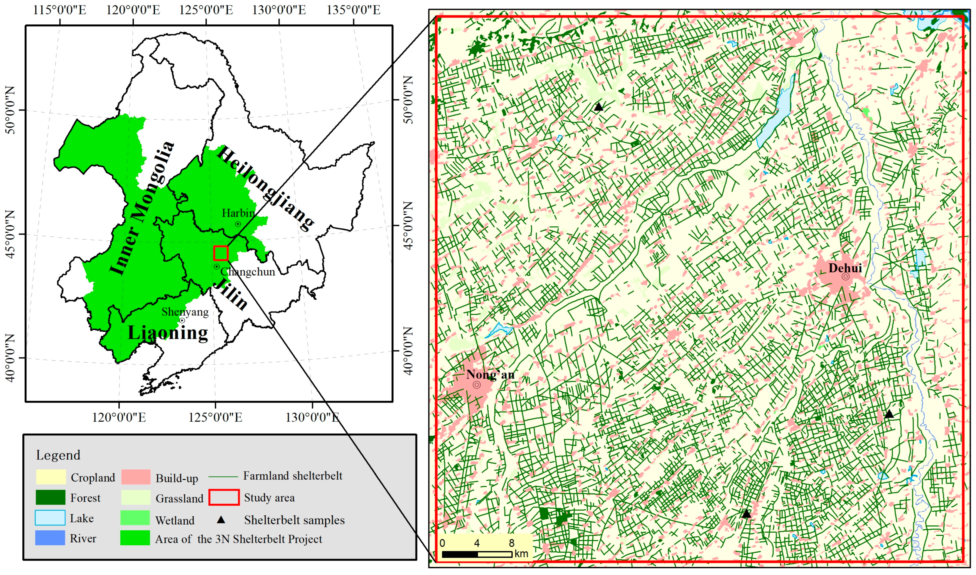
Figure 2.
Temporal distribution (day of year) of Landsat images (path: 118, row: 029) used in this study.
Figure 2.
Temporal distribution (day of year) of Landsat images (path: 118, row: 029) used in this study.
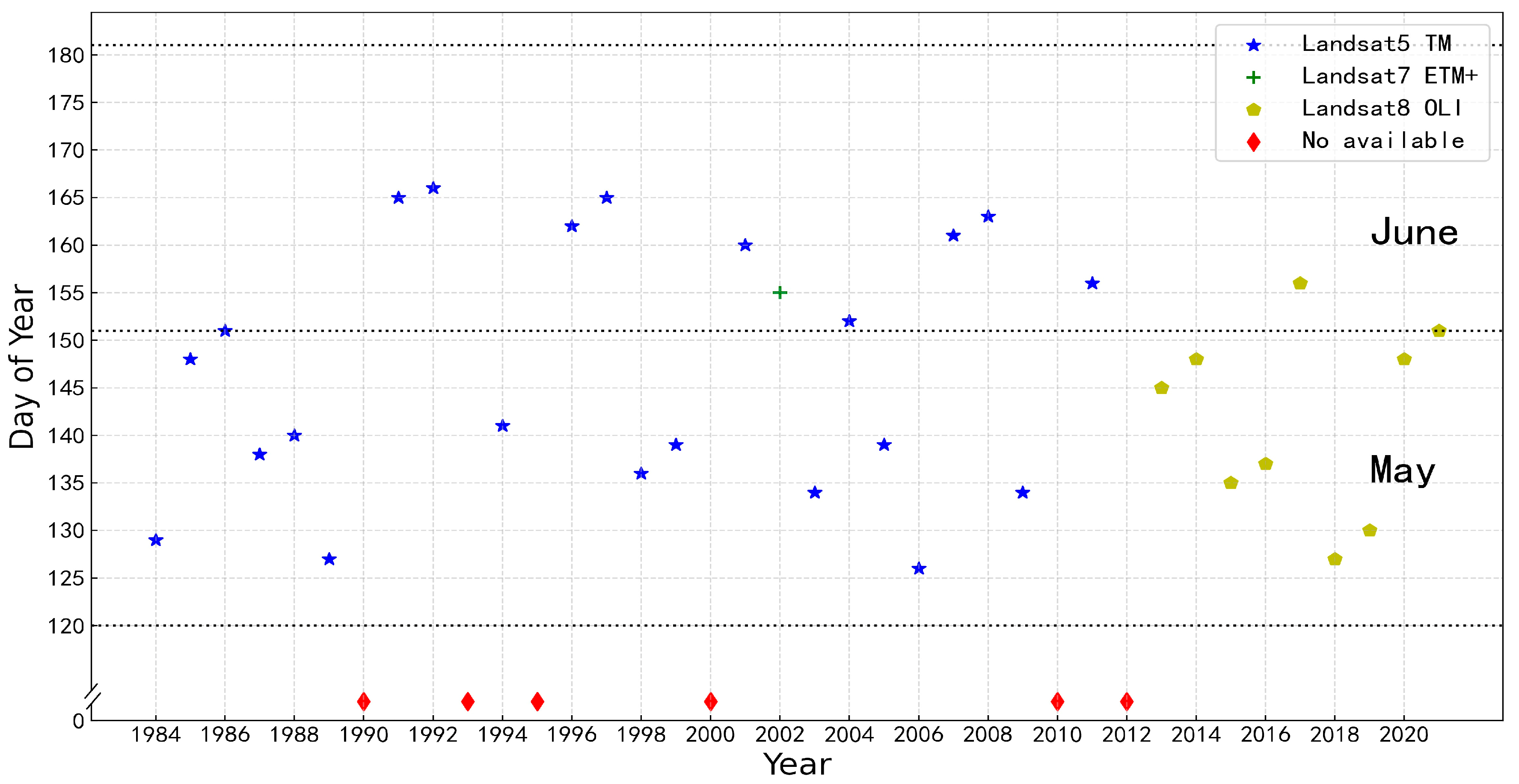
Figure 3.
(a) Landsat8 OLI image; the black line is the interpreted shelterbelt, the points are the extracted shelterbelt waveform values, and the red points are the valid values of the calculated FCFS. (b) The corresponding Google Earth Pro image of the shelterbelt. (c) The extracted maximum waveform of FCFS values. The red line is the mean value of the maximum waveform sequence.
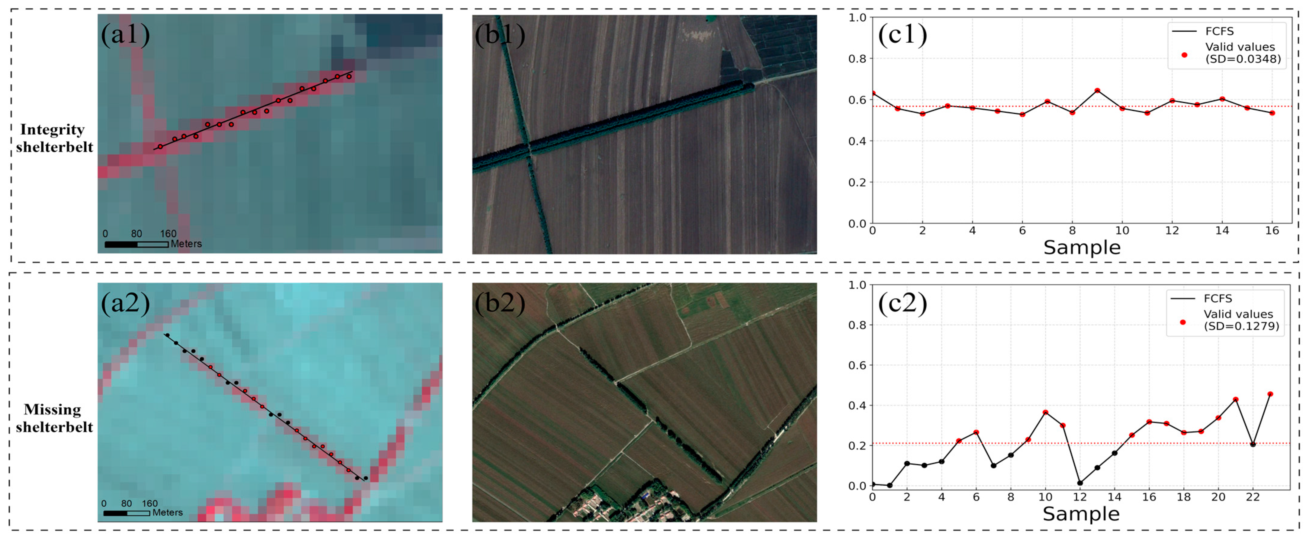
Figure 4.
Distribution of FCFS values at one-year intervals in different shelterbelts.
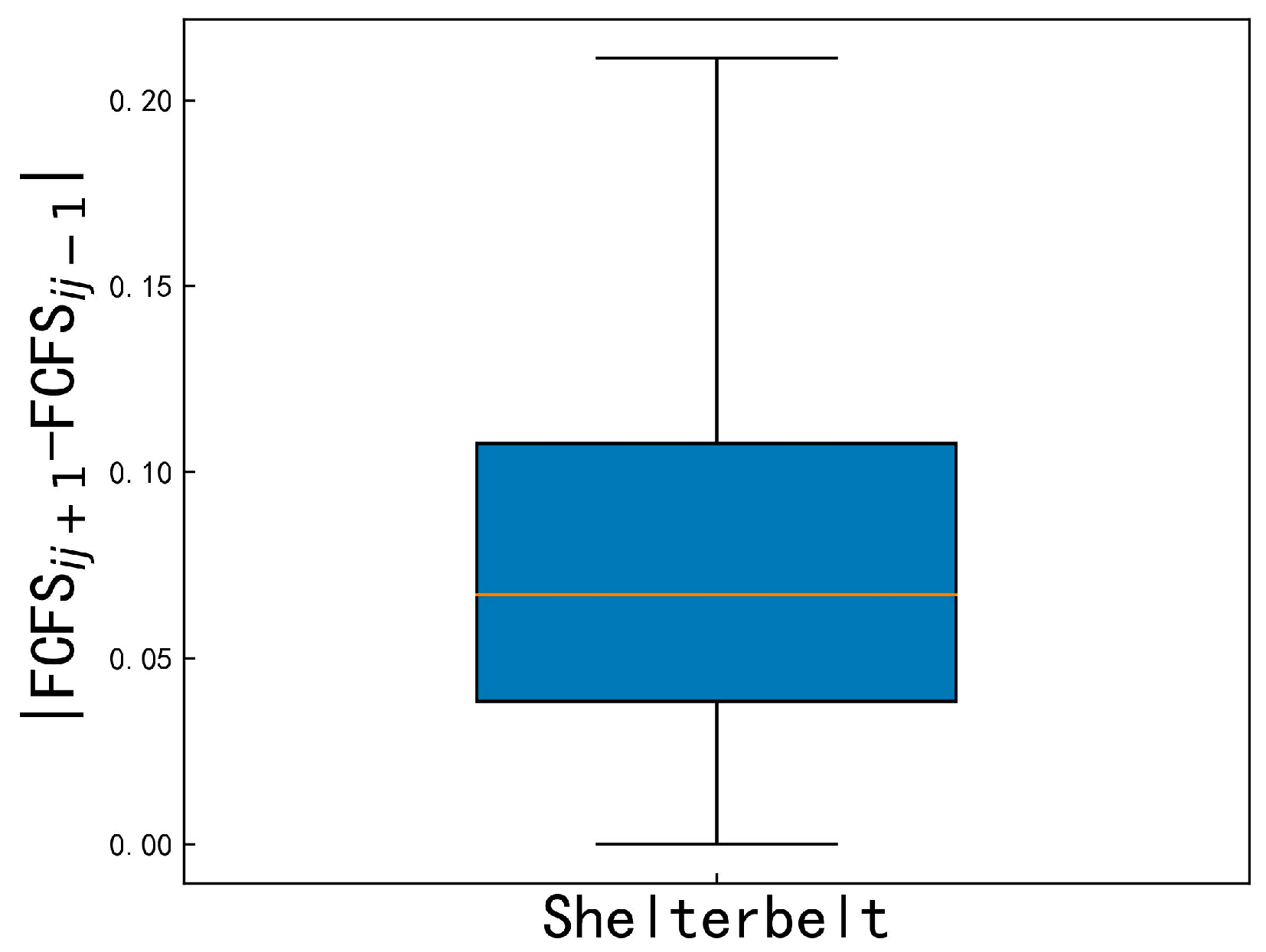
Figure 5.
Fractional coverage value of the shelterbelt (2–4 years) and cropland.
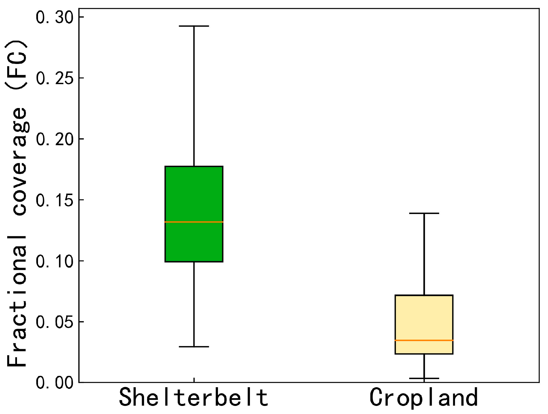
Figure 6.
(a) The annual growth process of the shelterbelt in Landsat (red: near-infrared band; green: red band; blue: green band). (b) The FCFS curve of the shelterbelt.
Figure 6.
(a) The annual growth process of the shelterbelt in Landsat (red: near-infrared band; green: red band; blue: green band). (b) The FCFS curve of the shelterbelt.
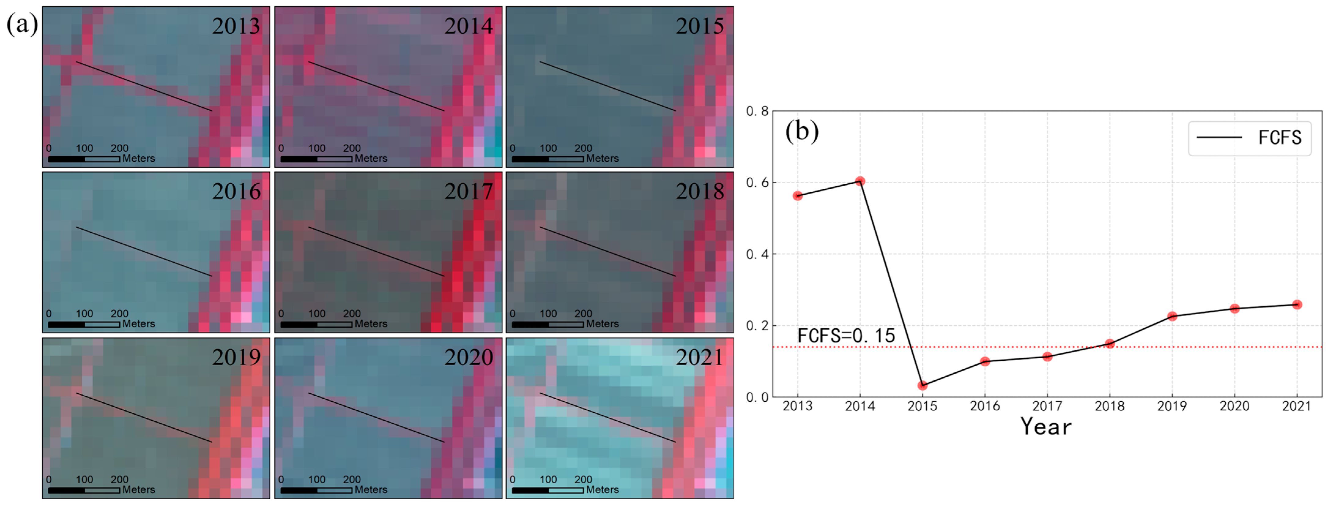
Figure 7.
Simulation curve of FCFS for different growth patterns; the red line is FCFS = 0.15 as the initial recognition threshold of shelterbelt.
Figure 7.
Simulation curve of FCFS for different growth patterns; the red line is FCFS = 0.15 as the initial recognition threshold of shelterbelt.

Figure 8.
(a) The linear relationship between the truth FCFS and the FCFS obtained through the dimidiate pixel model inversion. (b) The sample changing trend of truth FCFS and FCFS obtained through the dimidiate pixel model inversion.
Figure 8.
(a) The linear relationship between the truth FCFS and the FCFS obtained through the dimidiate pixel model inversion. (b) The sample changing trend of truth FCFS and FCFS obtained through the dimidiate pixel model inversion.

Figure 9.
(a) Total accuracy varies with permissible error age (year). (b) The accuracy varies across different age phases.
Figure 9.
(a) Total accuracy varies with permissible error age (year). (b) The accuracy varies across different age phases.
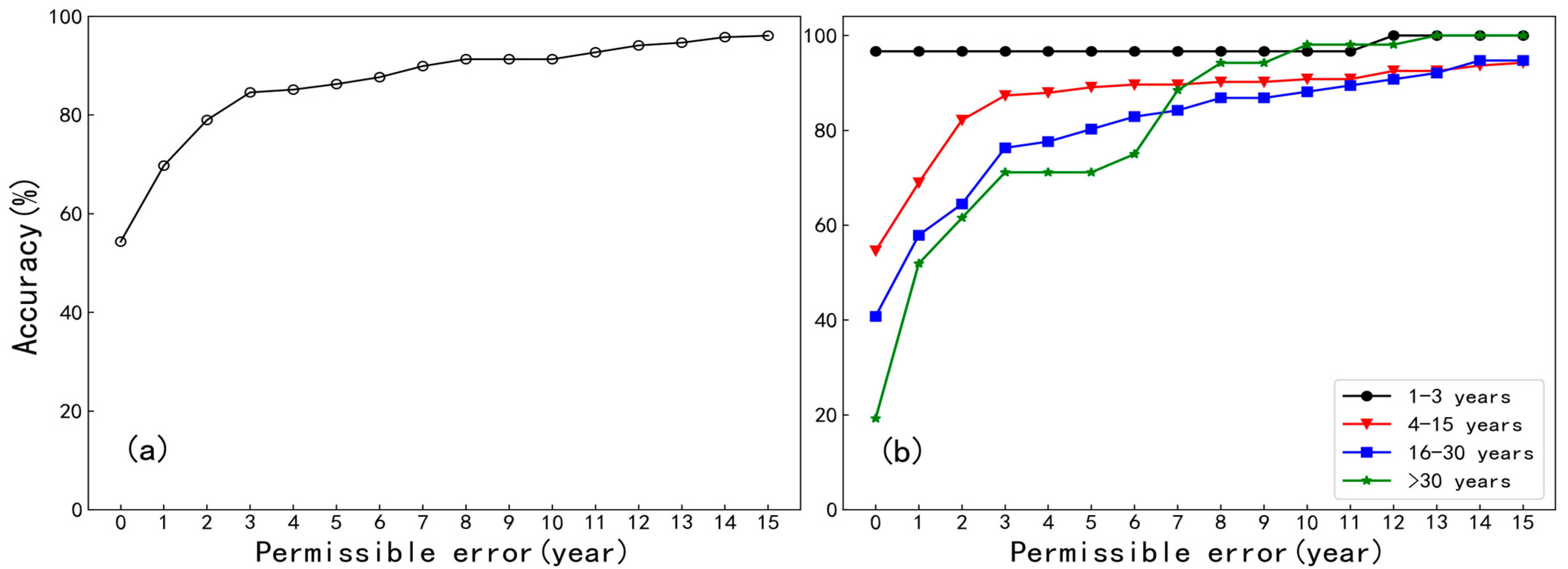
Figure 10.
Age spatial distribution of the shelterbelt in the study area (2021).
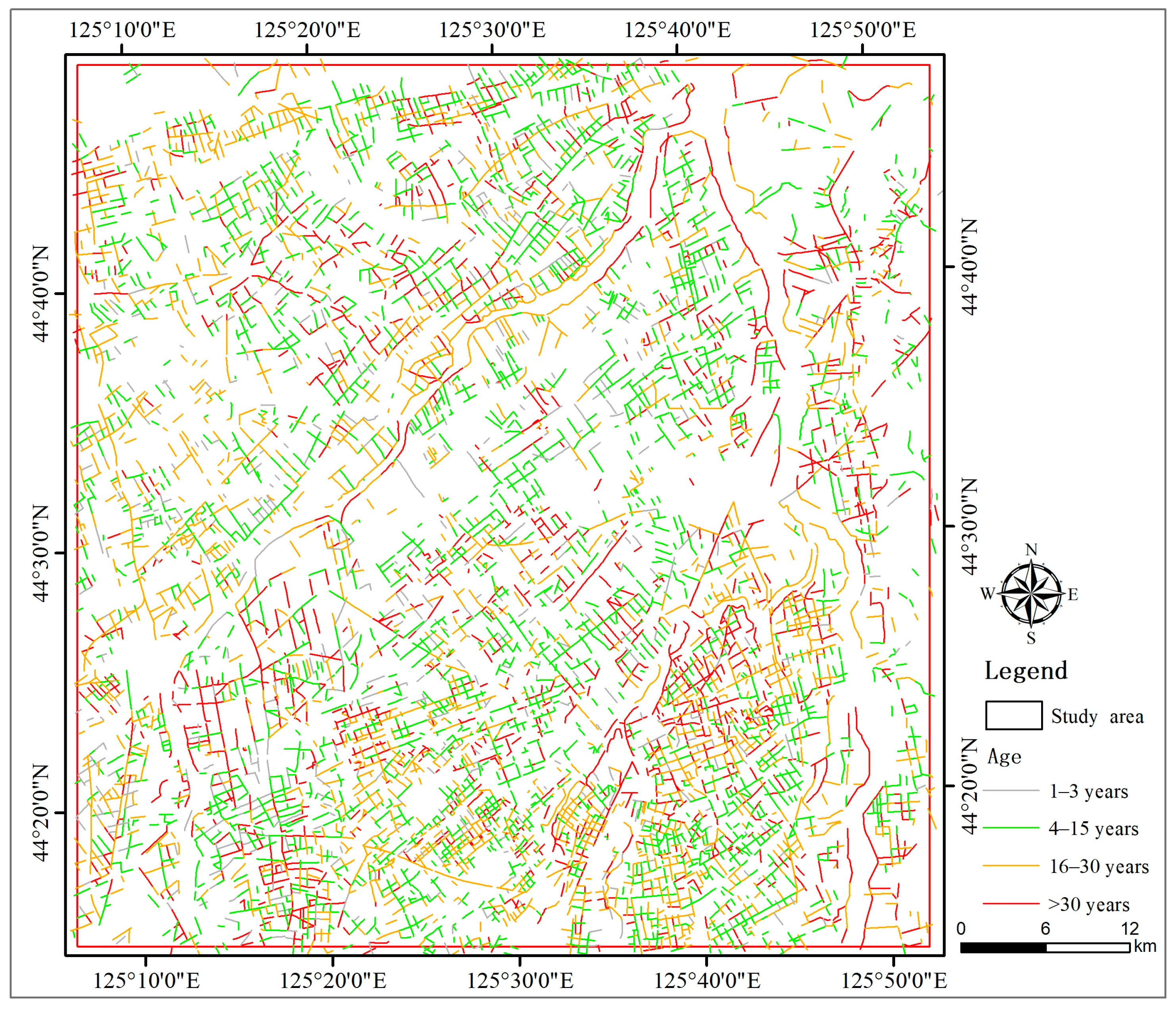
Figure 11.
Statistical diagram of age and growth pattern of shelterbelt in the study area. (a) The proportions of different age phases. (b) Proportions of different growth patterns. (c) The proportion of growth patterns corresponding to different age phases.
Figure 11.
Statistical diagram of age and growth pattern of shelterbelt in the study area. (a) The proportions of different age phases. (b) Proportions of different growth patterns. (c) The proportion of growth patterns corresponding to different age phases.


Table 1.
Confusion matrix between extracted and truth age. Overall accuracy = 85.15%.
| Truth Age | |||||||
|---|---|---|---|---|---|---|---|
| Phases | 1–3 Years | 4–15 Years | 16–30 Years | >30 Years | Total | Commission | |
| Extracted age | 1–3 years | 59 | 6 | 5 | 0 | 70 | 0.1571 |
| 4–15 years | 1 | 151 | 6 | 0 | 158 | 0.0443 | |
| 16–30 years | 0 | 13 | 64 | 17 | 94 | 0.3191 | |
| >30 years | 0 | 4 | 1 | 30 | 35 | 0.1428 | |
| Total | 60 | 174 | 76 | 47 | 357 | ||
| Omission | 0.0166 | 0.1321 | 0.1578 | 0.3617 | |||
Disclaimer/Publisher’s Note: The statements, opinions and data contained in all publications are solely those of the individual author(s) and contributor(s) and not of MDPI and/or the editor(s). MDPI and/or the editor(s) disclaim responsibility for any injury to people or property resulting from any ideas, methods, instructions or products referred to in the content. |
© 2023 by the authors. Licensee MDPI, Basel, Switzerland. This article is an open access article distributed under the terms and conditions of the Creative Commons Attribution (CC BY) license (https://creativecommons.org/licenses/by/4.0/).
Share and Cite
MDPI and ACS Style
Zhang, X.; Li, J.; Li, Y.; Deng, R.; Yang, G.; Tang, J. Age Identification of Farmland Shelterbelt Using Growth Pattern Based on Landsat Time Series Images. Remote Sens. 2023, 15, 4750. https://doi.org/10.3390/rs15194750
AMA Style
Zhang X, Li J, Li Y, Deng R, Yang G, Tang J. Age Identification of Farmland Shelterbelt Using Growth Pattern Based on Landsat Time Series Images. Remote Sensing. 2023; 15(19):4750. https://doi.org/10.3390/rs15194750
Chicago/Turabian StyleZhang, Xing, Jieling Li, Ying Li, Rongxin Deng, Gao Yang, and Jing Tang. 2023. "Age Identification of Farmland Shelterbelt Using Growth Pattern Based on Landsat Time Series Images" Remote Sensing 15, no. 19: 4750. https://doi.org/10.3390/rs15194750
Note that from the first issue of 2016, this journal uses article numbers instead of page numbers. See further details here.