Spatiotemporal Evolutions of the Suspended Particulate Matter in the Yellow River Estuary, Bohai Sea and Characterized by Gaofen Imagery

Abstract

Suspended particulate matter is a crucial component in estuaries and coastal oceans, and a key parameter for evaluating their water quality. The Bohai Sea, a huge marginal sea covering an expanse of 77,000 km² and constantly fed by numerous sediment-laden rivers, has maintained a high level of total suspended particulate matter (TSM). Despite the widespread development and application of TSM retrieval algorithms using commonly available satellite data like Landsat, Sentinel, and MODIS, developing TSM retrieval algorithms for China’s Gaofen (GF) series (GF-6 and GF-1) in the Bohai Sea is still a great challenge, mainly due to the limited applicability of empirical algorithms. In this study, 259 in situ measured-TSM samples were collected for algorithm development. The remote sensing reflectance (R_rs) curve demonstrates prominent peaks between 550 and 580 nm. Through conversion to remote sensing reflectance, it was found that single-band data had a weak correlation with TSM, reaching a maximum correlation of 0.44. However, by combining bands of band ratio calculations, the correlation was enhanced. Particularly, the blue and green band equivalent R_rs ratio had a correlation coefficient of 0.81 with TSM, and the proposed TSM inversion exponential algorithm developed based on this factor obtained an R-squared (R²) value of 0.76 and a mean relative error (MRE) of 32.24%. Analysis results indicated that: (1) there are spatial variations in the TSM within the Bohai Sea, Laizhou Bay, and the Yellow River estuary, with higher levels near the coast and lower levels in open waters. The Yellow River estuary experiences seasonal fluctuations higher TSM during spring and winter, and lower variations during summer and autumn, and (2) the dynamics of TSM are affected by Yellow River runoff, with increased runoff leads to higher TSM levels and expanded turbid zones. This study proposes a new algorithm to quantify TSM evolutions and distributions in the Bohai Sea and adjacent regions using China’s Gaofen imageries.

1. Introduction

Suspended sediment is an important factor that directly affects ocean color, and its concentration and transparency have a large impact on the ocean water column [1,2,3,4]. The total suspended particulate matter (TSM) changes rapidly due to ocean dynamics and other factors, such as precipitation, runoff, extreme weather, etc. The Bohai Sea is a vital component of China’s continental shelf, and it receives sediment transports from major rivers like the Yellow River, Liaohe River, and Haihe River. Investigating and quantifying the spatiotemporal dynamics of TSM in the Bohai Sea is important for ecological environmental preservation, ocean sustainable development, and for guiding the planning and location selection for coastal environmental projects in the Bohai Sea area [5,6,7]. The conventional methods for monitoring and analyzing TSM consume a lot of human and material resources, and require certain hydroclimatic conditions, resulting in extensive time and effort. With the integration of remote sensing technology and the widespread utilization of satellite sensing systems including NASA’s Landsat, ESA’s Sentinel, China’s Gaofen (GF), and Korea’s GOCI, the abundant data from these diverse satellite sources provide ample resources for advancing ocean water color remote sensing [8,9,10,11,12,13,14]. Currently, China’s landcover satellite images with a resolution of 2 m and cloud cover of less than 20% have an annual land coverage of 99.8%, and the satellite images with a resolution of 16 m have a coverage of about 99.9%.

With the continuing advancement in remote sensing technology, suspended sediment monitoring methods have evolved to incorporate more mature physical models, empirical models, and semi-empirical models [2,15,16,17]. Among these methods, analytical models, rooted in rigorous radiative transfer theory, have a great application potential. However, the limitations of accurately determining inherent optical properties such as absorption coefficients and backscattering coefficients for various components in water bodies hinder the widespread use of this approach. Meanwhile, empirical and semi-analytical models rely on data sources that are more readily available and thus have been extensively used.

By analyzing TSM and satellite based spectral data, researchers have identified a strong correlation, which motivates the use of satellite data for TSM inversion [18]. Further, Landsat MSS and TM data have been routinely used to map TSM in the Yellow River estuary and the Gulf of Mexico [19,20]. Subsequent studies introduced hybrid spectral partitioning techniques and semi-analytical models to formulate inversion equations for TSM in diverse regions. Additionally, researchers have investigated temporal variations in the TSM along the western coast of India, considering pre- and post-monsoon TSM variations [21,22]. Empirical algorithms have revealed that the near-infrared (NIR) and thermal bands of the Landsat TM sensor exhibit strong correlations with TSM [23]. Moreover, the blue band/NIR (Near Infrared) band combination has been considered effective in constructing TSM algorithms [24]. However, due to variations in band configurations across different sensors, the selection and combination of bands for constructing TSM algorithms for the Gaofen image data remain challenging.

Along the Chinese coast, studies based on MODIS data have found that TSM variations in the southern Bohai Sea were closely related to winter littoral currents [25]. However, in the Yellow River estuary, the primary cause of the TSM dynamics was the re-suspension of shallow marine sediments [26]. Short-term suspended sediment results derived from GOCI data demonstrated a pronounced correlation between TSM and tides in strong tidal estuaries, including the Hangzhou Bay, especially during the flood and ebb tide phases of the high-tide period [1,4]. A similar pattern was corroborated by Gaofen-4 observations in the Pearl River Estuary [27]. These studies emphasized the divergent driving factors behind TSM variations in different coastal ocean regions. Especially, for the Bohai Sea region, where a comprehensive understanding of the spatiotemporal TSM variations remain elusive.

Here, we propose to employ Gaofen-6 (GF-6) and Gaofen-1 (GF-1) satellite data in combination with the in situ measured TSM and spectral data to identify suitable bands or optimal remote sensing parameters for constructing the TSM algorithm. Finally, this paper proposes a new algorithm to quantify TSM evolutions and distributions in the Bohai Sea and other regions using China’s GF-1 and GF-6 images.

2. Study Area and Data Prepare

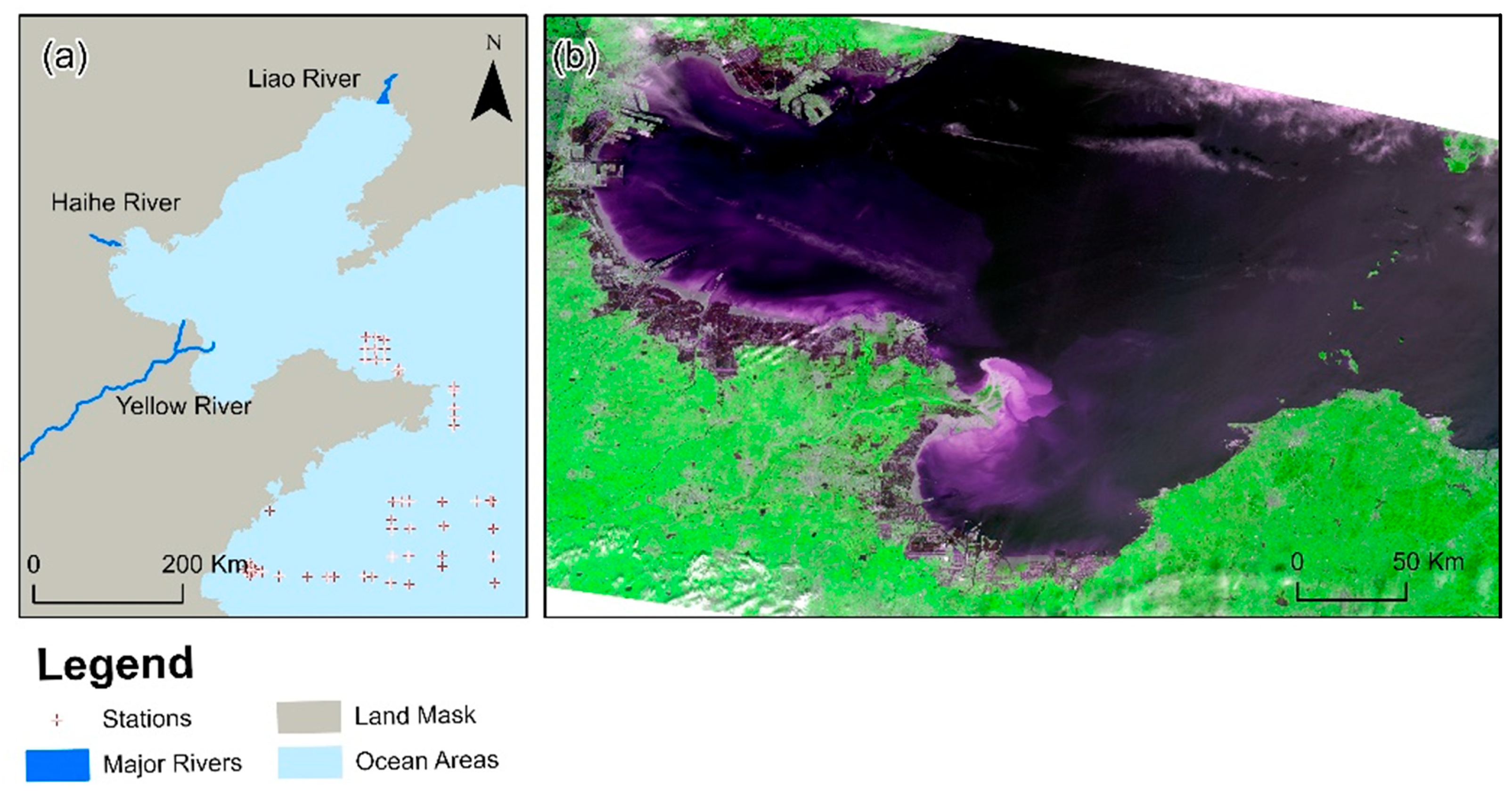
2.1. Overview of the Study Area

The Bohai Sea is a semi-enclosed inland sea at the mouth of the Yellow River in China, and it is situated in the southwest region (37°15′~38°10′N, 118°10′~119°15′E). It is a vast, shallow, and turbid water body, with an average depth of about 18 m. However, its inherent self-purification capacity is limited. With the rapid growth of industrialization and the impact of human activities, river runoff into the sea has decreased substantially. This reduction impedes the dilution of pollutants, leading to an increase in polluted sediments and severe degradation of the water environment. Meanwhile, the Bohai Sea region has rich marine biocultural, mineral farming, and salt marine resources. The total marine bioculture production alone constitutes about 40.9% of the national mariculture production in the current five-year period.

Within the Bohai Sea, the Yellow River is the primary contributor of sediment, with its estuary (37°59′–37°91′N, 119°09′–119°39′E) serving as the intersection between the Bohai Sea and Laizhou Bay. Most of the water in the Yellow River estuary is less than 10 m deep, and it becomes deeper and deeper as it moves offshore. Notably, the Yellow River is the river with the highest sediment content in the world, annually carrying substantial suspended sediment and various nutrient salts into the sea. The relatively slow flow velocity of the Yellow River can result in material deposition at its mouth.

Over the past two decades, rapid economic development and significant anthropogenic influences in the drainage area have led to increased sewage industrial wastewater discharges, and excessive runoff of agricultural fertilizerse. This has caused severe eutrophication in the seawater near the mouth of the Yellow River, as well as in the waters of Laizhou Bay and Bohai Bay. Apart from the Yellow River, which serves as the primary sediment source for the Bohai Sea, other rivers, such as the Haihe River and Liao River also contribute sediment resources to the Bohai Sea (Figure 1).

The Yellow River transports a large amount of terrestrial material into the Bohai Sea every year. As the largest river discharging into the Bohai Sea, the Yellow River contributes over half of the total river flow, and it transports a staggering 420 × 10⁸ m³ sediment every year. The mouth of the Yellow River constitutes a classic high-turbidity estuary, characterized by an enormous sediment discharge into the sea. Most of the marine sediment from the Yellow River is deposited near the estuary. Thus, this paper aims to develop a TSM algorithm encompassing the entire Bohai Sea, with a specific focus on the Yellow River estuary as a representative area for investigating the seasonal variations in TSM.

2.2. Data Acquisition

GF-6 and GF-1 wide field of view (WFV) image data were utilized in this study (See

Table 1. Sensor parameter settings.

Sensor	Band	Spectral Range/μm	Resolution/m
GF-1/GF-6 WFV	Band 1 (Blue)	0.45–0.52	16
	Band 2 (Green)	0.52–0.59
	Band 3 (Red)	0.63–0.69
	Band 4 (NIR)	0.77–0.89

for sensor parameter settings). All the GF data were downloaded from the website of the China Resources Satellite Application Center (http://www.cresda.com, accessed on 4 September 2020, 9 March 2021, 24 July 2021, 27 November 2021 and 9 February 2021). In this study, in situ sampled TSM data were collected from 64 fixed stations and 25 continuous stations, with a total of 249 samples for analysis in 2017. Specifically, the data from 21 stations were simultaneously analyzed to obtain both TSM data and surface spectral reflectance data. The observation equipment and setup are in line with internationally recognized observational standards.

2.2.1. Spectral Data

The Field Spec3 spectroscopy instrument with a spectral range of 350–2500 nm is manufactured by ASD (Analytical Spectral Devices, Inc., Boulder, CO, USA). Measurements were conducted following NASA ocean optics specifications, with an observation angle of (40°, 135°). Here, 40° denotes the angle between the instrument probe and the sea surface normal direction, and 135° denotes the angle between the instrument observation plane and the solar incidence plane. According to the above-water method [28], the remote sensing reflectance R_rs can be calculated using the following equation:

$$R_{rs}=\frac{(L_u-{\rho }_f\times L_{sky})\times {\rho }_P}{\pi \times L_P}$$

(1)

where $L_u$, $L_{sky}$, and $L_P$ represent the measured signals when the spectrometer measures the water, sky, and standard plate, respectively; ${\rho }_f$ represents the Fresnel reflectance (the magnitude of its value is related to the wind speed).

Each station’s data includes records of the respective station name, measurement date and time, wind speed, wind direction, temperature, pressure, cloud cover, sea state, and light variation. After the relative deviation of spectral reflectance for each station was calculated, the spectral data were meticulously screened, and stations with a relative deviation of less than 5% were selected. In this study, after screening the corresponding concentration data, 39 pairs of in situ data or ground-truth measurements were obtained, including both TSM and spectral data.

2.2.2. Processing of the In Situ TSM Data

The Whatman GF/F 0.7 μm glass fiber filter papers were used for water sample filtration. After the water samples were filtered, the membranes were placed in an oven and dried at a constant temperature of 105 °C. The first drying time was 24 h, and the subsequent drying time was only 4 h. After drying, the membranes were cooled in a desiccator for at least 4 h to return to room temperature and then weighed. Each membrane was weighed several times until the difference between two consecutive weightings was within 0.1 mg/L. The membrane was weighed several times until the difference between two consecutive weightings was within 0.1 mg/L. Finally, the concentration of TSM including inorganic and organic suspended matter was measured.

2.2.3. Remote Sensing Data Processing

Considering the spatial offset in the GF satellite imagery, this study initiated a georeferencing process upon data acquisition to pinpoint accurate ground control points, thereby complementing the high-resolution remote sensing data. Meanwhile, radiometric calibration, terrain correction, and other essential procedures were conducted. Following these steps, the FLAASH model for atmospheric correction was implemented, resulting in the derivation of remote sensing reflectance. In this case, both the mean (AVG) and standard deviation (STD) of remote sensing reflectance were computed. Specifically, only the data falling within the range of AVG–3STD to AVG + 3STD were retained, while null data were excluded through median filtering. This preparatory work greatly facilitated subsequent analysis and processing.

3. TSM Algorithm Establishment

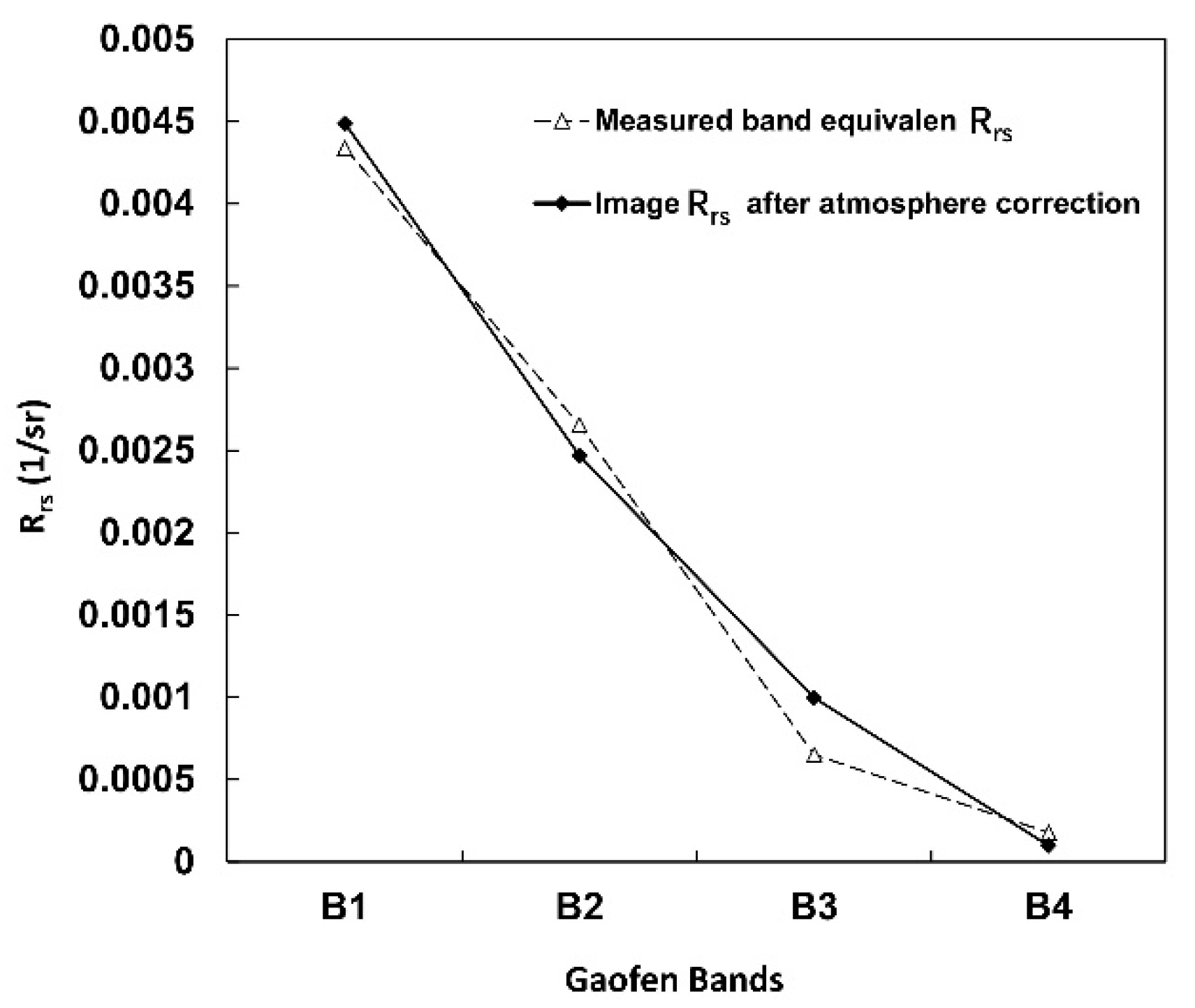
3.1. Validation of the Atmospheric Correction

A comparison was conducted between the GF-6 Blue (B1), Green (B2), Red (B3), and NIR (B4) band remote sensing reflectance data and the FLAASH atmospherically corrected remote sensing reflectance data to evaluate the accuracy and suitability of the atmospheric correction method (Figure 2). Some detailed information regarding the validation against in situ data can be found in Hu et al. [1].

The results indicate that the FLAASH model yields more accurate outcomes in the B1 and B2 bands, with relative errors of 3.42% and 7.02%, respectively. In contrast, the model performs less effectively in the B3 and B4 bands, with relative errors of 53.32% and 44.64%, respectively. Thus, this study only considered the B1 and B2 bands in the algorithm construction process for subsequent research.

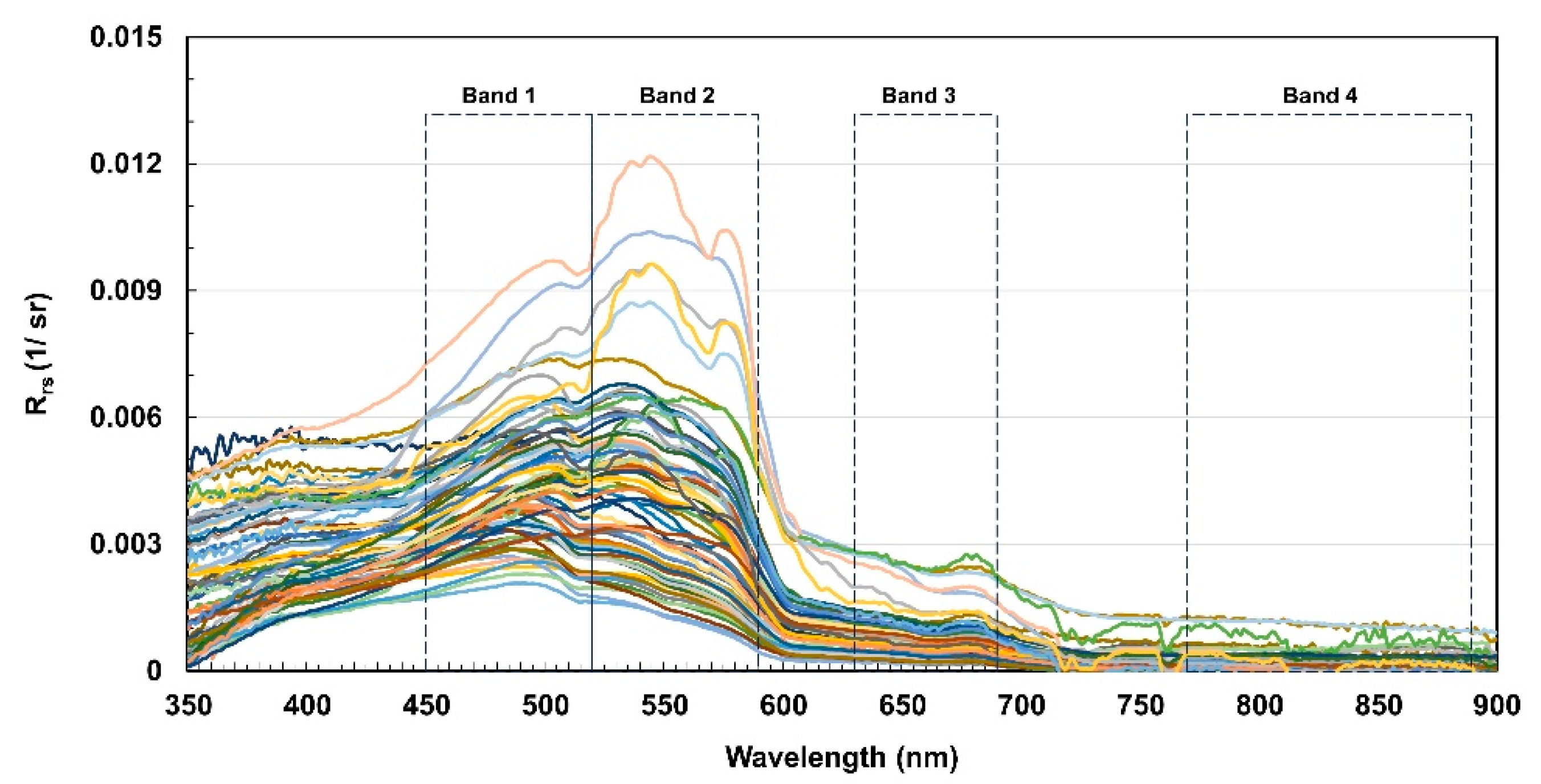
3.2. Characterization of Spectral Data and Equivalent Remote Sensing Reflectance

The measured remote sensing reflectance data and the GF-6/GF-1 band settings for water bodies in Bohai Bay are shown in Figure 3. There is an evident peak around 570 nm, exhibiting a ‘broad peak’ shape with a tendency to shift toward the red portion of the spectrum, and this is commonly referred to as the ‘redshift’ phenomenon. The peak reflectance in the visible wavelength range appears around 580 nm, followed by a rapid decline in reflectance beyond the peak wavelength, as wavelengths exceed 600 nm. In the range of 600–700 nm, the reduction in reflectance is relatively gradual, with the reflectance reaching its nadir around 670 nm due to phytoplankton absorption. Generally, spectral reflectance increases with the rise in suspended matter content, and the peak wavelength experiences a red-ward shift.

By utilizing the spectral response function, the measured spectral data were converted to GF equivalent remote sensing reflectance for each band. Through this process, 39 data pairs were obtained. The calculation of GF equivalent remote sensing reflectance is shown below:

$$R_{rsi}=\frac{{\int }_{{\lambda }_1}^{{\lambda }_2}{S}_i\left(\lambda \right)R_{rs}\left(\lambda \right)d\lambda }{{\int }_{{\lambda }_1}^{{\lambda }_2}{S}_i\left(\lambda \right)d\lambda }$$

(2)

where, R_rsi denotes the equivalent remote sensing reflectance, S_i denotes the spectral response function of the adopted image, and R_rs denotes the measured remote sensing reflectance at each station. The wavelength λ₁ and λ₂ correspond to the response points on both sides of the response function.

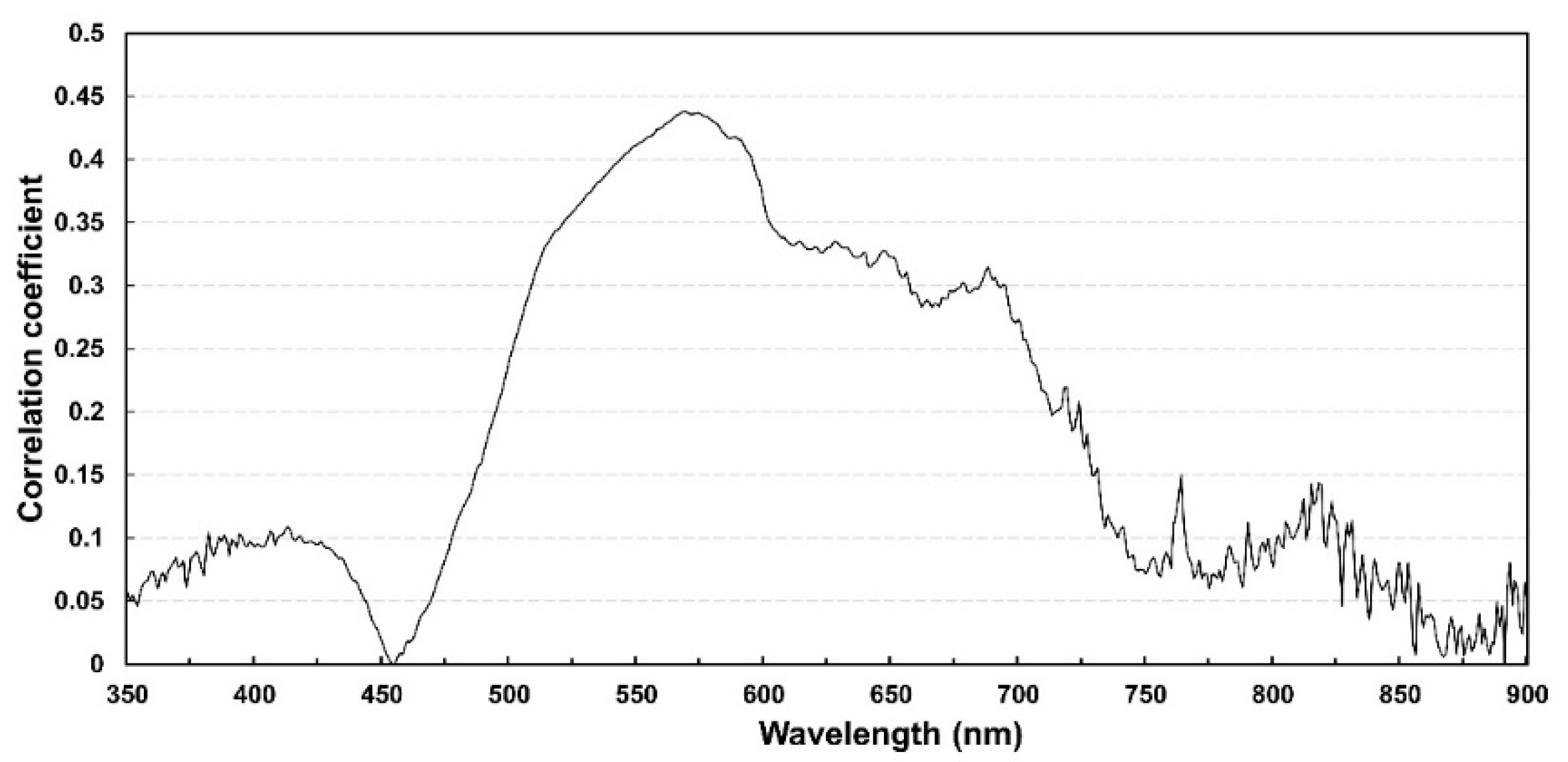
3.3. Bands Sensitive Analysis and TSM Inversion Algorithm

The Pearson correlation coefficient (Equation (3)) was calculated to analyze the correlation of remote sensing reflectance of water bodies corresponding to the TSM data, and the correlation was analyzed to select sensitive wavebands for subsequent modeling.

$$r_{xy}=\frac{\sum _{i=1}^n\left(x_i-\overline{x}\right)\left(y_i-\overline{y}\right)}{\sqrt{\sum _{i=1}^n\left(x_i-\overline{x}\right)}\sqrt[2]{\sum _{i=1}^n{\left(y_i-\overline{y}\right)}^2}}$$

(3)

where, $r_{xy}$ denotes the correlation coefficient of remote sensing reflectance; $x_i$ and $y_i$ are two variables, and the three $x$ variables, namely, single band, band difference, and band ratio, are used to derive the most correlated $x$ variable; $\overline{x}$ and $\overline{y}$ represent the means of the two variables, respectively. The closer the value of $\left|r_{xy}\right|$ is to 1, the stronger the correlation.

The results (Figure 4) demonstrate that the correlation coefficient increases significantly within the wavelength range of 480–580 nm, with the highest correlation coefficient being observed near 570 nm. Consequently, the correlation coefficient between this measured spectral data and TSM continues to increase across the B1 and B2 bands. Hence, our data modeling efforts focused on these two bands.

The in situ dataset consisting of 39 measurements was utilized to develop the TSM classification algorithm. Two-thirds of this dataset was used to model construction, while the remaining one-third was used for result verification. To establish the inversion algorithms connecting remote sensing factors and TSM, four functional models were developed: exponential, logarithmic, linear, and power functions. Subsequently, the coefficient of determination (R²), root mean square error (RMSE), and mean relative error (MRE) were computed to evaluate the performance of the TSM algorithm.

Specifically, based on the data of the B1 and B2 bands, difference calculations, ratio operations, and combination operations were conducted for the two bands. For example, the blue and green band ratio had a correlation coefficient of 0.81 with TSM. Then, algorithms were constructed using linear, exponential, and power models. Notably, the R² values in

Table 2. Comparison with TSM inversion algorithms.

Models	Remote Sensing Factor (x)	TSM (y) Algorithm	R2
Linear Function	B2/B1	$y=7.05\ast x-3.39$	0.71
Exponential Function	B2/B1	$y=0.17\ast EXP(2.93\ast x)$	0.76
Power Function	B2/B1	$y=3.31\ast x^{2.43}$	0.74
Linear Function	(B2–B1)/(B2/B1)	$y=0.014\ast x+3.68$	0.53
Exponential Function	(B2–B1)/(B2/B1)	$y=3.23\ast EXP(0.0059\ast x)$	0.60
Polynomial Function	(B2–B1)/(B2/B1)	$y={10}^{-4}\ast x^2+0.03\ast x+3.58$	0.68
Linear Function	B2–B1	$y=1781.60\ast x+3.63$	0.74
Exponential Function	B2–B1	$y=3.16\ast EXP(741\ast x)$	0.75
Polynomial Function	B2–B1	$y=\mathrm{340,830}\ast x^2+2092.70\ast x+3.4$5	0.75

indicated that the exponential model with B2/B1 as the remote sensing factor and the exponential model with (B2–B1) as the remote sensing factor obtained high coefficients of determination, which were 0.76 and 0.75, respectively. Further, the validation dataset was applied to these two algorithms, and the exponential model with B2/B1 as the remote sensing factor outperformed the other two models in both RMSE and MRE metrics. Thus, this algorithm was selected to calculate the TSM in the Bohai Sea in the following equation:

$$\mathrm{T}\mathrm{S}\mathrm{M}=0.17\ast \mathrm{E}\mathrm{X}\mathrm{P}(2.93\ast \mathrm{X})$$

(4)

where X = R_rs(B2)/R_rs(B1).

4. Results and Discussion

4.1. The Spatial TSM Distribution in the Bohai Sea

The GF-6 image data used in this study was acquired on 4 September 2020. Before mapping the TSM distribution, the normalized difference water index (NDWI) was employed to distinguish between water bodies and land. A threshold of −0.1 was set for water and land extraction, where regions with NDWI values larger than −0.1 were classified as water bodies, and those with NDWI values smaller than −0.1 were classified as land. Only the regions classified as water bodies were used for TSM mapping.

By using the inversion algorithm, the results in Figure 5 indicate that the Bohai Sea generally exhibits higher TSM concentration near the northern part of the bay as compared to the bay’s mouth. Meanwhile, the TSM concentration gradually decreases with the increasing distance from the shore. The TSM concentration in the near-shore waters is the highest, and this is primarily influenced by sediment transport from the Haihe River, which is the largest contributor to sand transport in Bohai Bay. Moreover, elevated TSM concentrations are particularly noticeable in Bohai Bay, Laizhou Bay, and the Yellow River estuary.

In Laizhou Bay, the highest TSM is observed in the surface layer of the southwestern sea area, and it is mainly sourced from the Yellow River. The mouth of the Yellow River exhibits the highest TSM, with a gradual decrease toward the middle. This demonstrates that, facilitated by the shallow waters, suspended sediment mainly settles in the near-shore area, making it susceptible to environmental influences. Furthermore, the development of near-shore industries leads to the transport of pollutants by suspended sediment in the water body.

4.2. Quantifying the Spatiotemporal Distribution of TSM in the Yellow River estuary

The Yellow River estuary, a typical high-turbidity estuary in China, was selected as a case study in this paper to further investigate the spatiotemporal distribution of TSM in this region. The retrieval algorithm was adopted to map the TSM in the Yellow River estuary using four high-quality GF-1 satellite images captured in 2021. These images were acquired on 9 March 2021 (spring), 24 July 2021 (summer), 27 November 2021 (fall), and 9 February 2021 (winter). The TSM distribution in the Yellow River estuary was classified based on seasons, and the results from each image were categorized as high, medium, or low (Figure 6).

Analysis shows that there are distinct patterns in the spatial and temporal distribution of TSM in the Yellow River estuary. The dry period of the Yellow River includes January, February, March, November, and December, characterized by minimal runoff and sand transport (Figure 7). In this period, the impact of runoff on suspended sediment near the mouth of the Yellow River is limited. Meanwhile, the flood season includes July, August, and September, with significantly higher water and sand transports from the Yellow River compared to other months. In this period, the residual flow of runoff becomes a crucial factor affecting sediment transport.

The TSM distribution pattern in the Yellow River estuary appears as stripes along the coastline, mainly extending southward into Laizhou Bay. Under various influencing factors, the extent of southward extension varies, and some sediment is also distributed from the estuary to the near-shore sea north of the Xiaoqing River. During spring and autumn, the volume of sand transported from the Yellow River is significantly higher than that in winter, albeit still lower than that during the flood season. The Bohai Sea experiences windy weather during spring and autumn, characterized by variable wind directions. The suspended sediment near the mouth of the Yellow River is the result of the combined action of Yellow River runoff and submarine sediment resuspension. Tides and residual currents play a role in transporting suspended sediment, and the high suspended sediment water range tends to contract toward the shore compared to that in the winter.

In recent years, many scholars have studied the Bohai Sea TSM models and retrieval results using different satellite data. For instance, Li et al. used GOCI images to retrieve the surface suspended sediment concentration in the Bohai Sea [29]. Cui et al. constructed a remote sensing inversion model of TSM using 555 and 670 nm band remote sensing reflectance based on the field-measured or in situ TSM and spectral data in Bohai Bay and Laizhou Bay [30]. Li et al. utilized Landsat 8 Operational Land Imager data to estimate the variation of TSM from 2013 to 2019, and a simple empirical algorithm was developed to map the TSM distribution with an MRE of 33.12% [31]. Compared with different sensor results, the Bohai Sea TSM retrieval distribution in this study is consistent with others. The annual average distribution of TSM suggests that the high turbid area of TSM Is mainly distributed around the Yellow River estuary, northwest of Laizhou Bay and the southern Bohai Bay; the impact of river runoff is mainly concentrated in the estuary. Meanwhile, the study indicates that the seasonal distribution of TSM varies greatly, and the range and intensity of TSM in winter are higher than those in summer.

4.3. Analysis of Factors Driving TSM Variations in the Yellow River Estuary

4.3.1. Wind, Wind Waves, and Storm Surge

During winter, the Bohai Sea usually experiences prevailing northerly and northwesterly winds with high wind speeds, occasional storm surges, and wave-induced sediment resuspension in shallow nearshore areas. This wave resuspension is an important source of suspended sediment in the sea. The strong north winds, combined with southward waves, generate a southward coastal current in the western delta of Laizhou Bay. This current transports suspended sediment southwestward along the west coast of Laizhou Bay and eventually toward the Bohai Strait. Under the influence of tides, the high-concentration water transported to Laizhou Bay is further transported to distant seas.

Through the generation of rift currents, wind and waves not only disturb shallow sediment but also carry fine sand directly from the shallow sea. This dynamic factor plays a crucial role in sediment movement and transport in the shallow sea. Meanwhile, wind and waves enhance the sea current’s ability to carry sediment. The prevailing wave direction in the Yellow River estuary is east to northeast (with a frequency of 29%), and the secondary wave direction is north to northwest (with a frequency of 18%). The strong wave directions include north-northeast and northeast, and secondary strong wave directions include north-northwest and northwest. The wind field affects the northern bank section of the Yellow River, making it more efficient in transporting sand to the west than the eastern bank section to the south. Also, sand transport capacity increases from the upper bay to the mouth of the bay. In the flood season, the sand transport capacity of the northern bank section to the west strengthens, while that of the eastern bank section to the south weakens.

Storm surges are common in Bohai Bay and Laizhou Bay, and they mainly occur in April and September due to a combination of regional wind patterns and geographical factors. These surges are mostly caused by extended periods of high winds, particularly northeasterly winds with speeds ranging from 17.2 to 24.5 m/s. The storm surges lead to a sudden rise in tide levels, typically 2–3 m higher than the normal high tide level. Meanwhile, storm surges have a significant impact on the distribution of suspended sediment, especially the resuspending bottom sediment in shallow nearshore areas.

4.3.2. Human Activities

Human activities mainly affect the distribution and dispersion of incoming sediment through changes in runoff volume and sand transport. Over the past 50 years, the Yellow River has experienced a reduction in marine sediment input, due to both climate change and anthropogenic activities within the basin.

Anthropogenic activities have significantly affected the Yellow River basin through soil and water conservation, irrigation, reservoir construction, etc., leading to a decline in marine sediment. Since the 1950s, comprehensive watershed management and soil conservation efforts have changed sub-basin conditions, reduced erosion intensity, and significantly decreased the amount of sediment reaching the estuary.

The main driving factor for reduced runoff is irrigation diversion. In the water diversion process, irrigation diversion will also divert sediment and reduce the amount of sediment inflow into the sea. When abundant water is diverted in non-abundant periods, the runoff into the sea can be interrupted. Since the 1970s, there have been long-term interruptions in downstream flow, further reducing sediment input.

During the 1990s, the Sanmenxia reservoir in the middle reaches of the Yellow River continued to release muddy water, which changed sediment distribution throughout the year. Although the runoff process remained largely unchanged, this practice changed sediment distribution, particularly during the flood season.

5. Conclusions

In this paper, by using the spectral and measured suspended particulate matter concentration data in the Bohai Sea in 2017, a TSM retrieval algorithm was established based on the Gaofen (GF) satellite images, and the spatiotemporal variations of the TSM in Yellow River estuary in 2021 were analyzed:

(1)

We quantified the evolution and spatiotemporal TSM variations in the Bohai Sea using a optimal classification algorithm developed using in situ measured TSM data applied on the GF-6/GF-1 satellite image data. The peak of the measured remote sensing reflectance in the Bohai Sea region appears near the wavelength of 580 nm. Based on the correlation analysis between the GF Band 1, Band 2, Band 3, and Band 4 equivalent remote sensing reflectance and the in situ measured-TSM and the atmospheric correction accuracy evaluation, an exponential model was established by taking the ratio of Band 1 and Band 2 equivalent remote sensing reflectance as the remote sensing factor, and the R² value of the model was 0.76. The inversion results suggest that the model can improve the characterization of the spatiotemporal distribution of TSM in the Bohai Sea region using GF images.

(2)

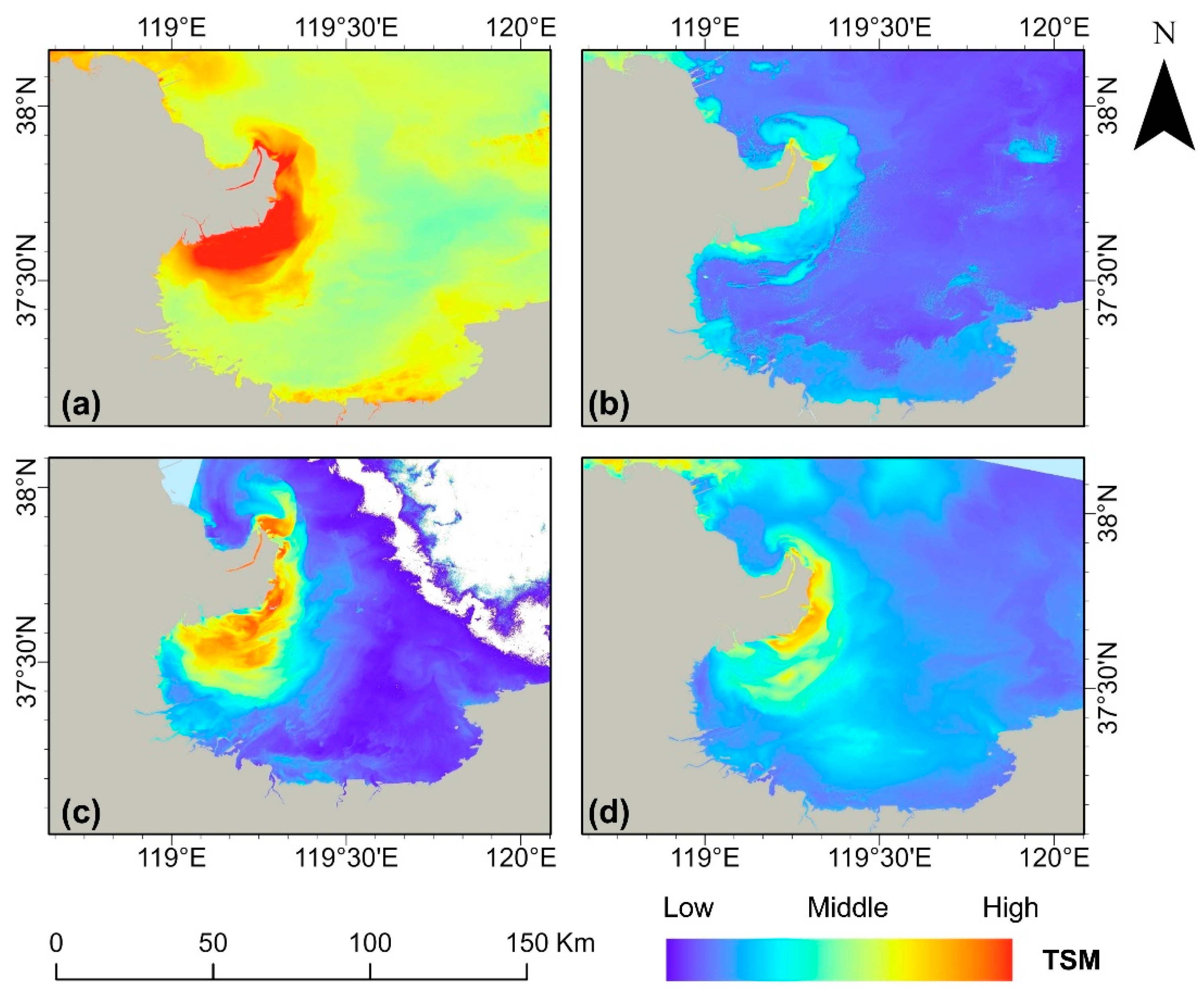
The spatiotemporal variations and the pattern distributions of the Yellow River estuary TSM was obvious. High TSM of water bodies was mainly concentrated in Bohai Bay, Laizhou Bay, and the Yellow River estuary near the sea, and the TSM was high near-shore and low offshore. The TSM in the Yellow River estuary sea showed an overall time distribution of being high in the spring and winter and low in summer and autumn.

(3)

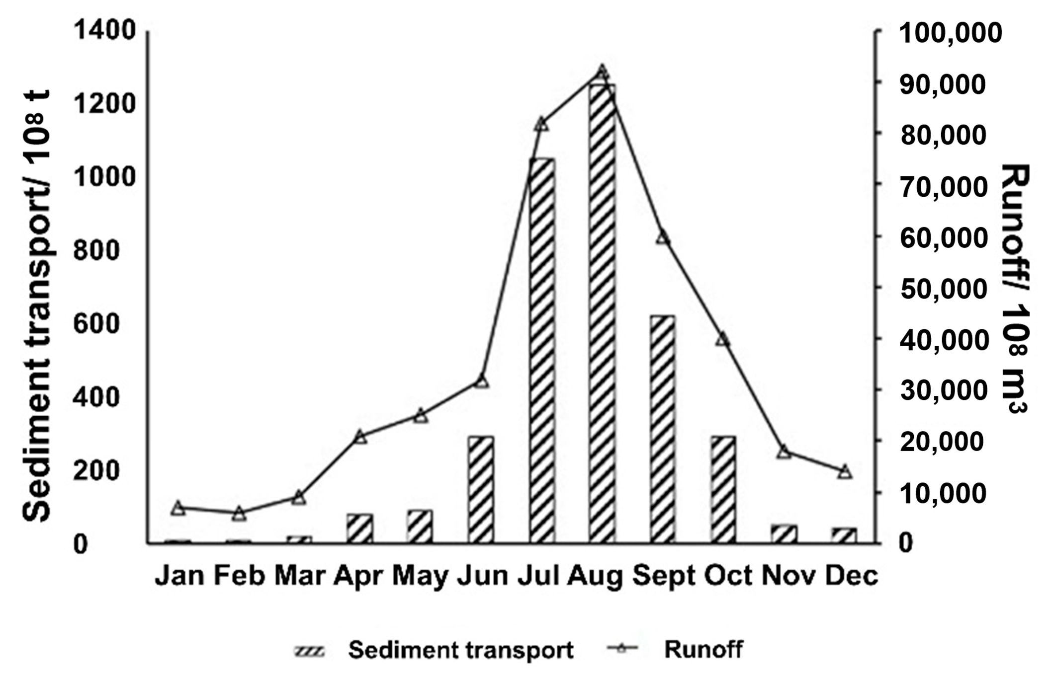
Yellow River runoff can affect the TSM in the Yellow River estuary. The Yellow River estuary carries a large amount of sediment into the Bohai Sea every year, and the area near the mouth of the Yellow River is affected by the Yellow River runoff; as the flow of the Yellow River runoff rises, the TSM concentration increases, so does the scope of influence. Bohai Bay and Laizhou Bay are less affected by the Yellow River runoff. This is because the sediment carried by the Yellow River runoff enters the Bohai Sea and then falls rapidly and is deposited mostly in the area near the mouth of the Yellow River; however, the deposited sediment is redistributed under the action of wind, tide, waves, and currents, and it can be transported to Bohai Bay, Laizhou Bay and other areas, and even into the Yellow Sea.

References

1. Hu, Y.; Yu, Z.; Zhou, B.; Li, Y.; Yin, S.; He, X.; Peng, X.; Shum, C.K. Tidal-Driven Variation of Suspended Sediment in Hangzhou Bay Based on GOCI Data. Int. J. Appl. Earth Obs. Geoinf. 2019, 82, 101920. [Google Scholar] [CrossRef]
2. He, X.; Bai, Y.; Pan, D.; Huang, N.; Dong, X.; Chen, J.; Chen, C.T.A.; Cui, Q. Using Geostationary Satellite Ocean Color Data to Map the Diurnal Dynamics of Suspended Particulate Matter in Coastal Waters. Remote Sens. Environ. 2013, 133, 225–239. [Google Scholar] [CrossRef]
3. He, X.; Bai, Y.; Pan, D.; Tang, J.; Wang, D. Atmospheric Correction of Satellite Ocean Color Imagery Using the Ultraviolet Wavelength for Highly Turbid Waters. Opt. Express 2012, 20, 20754. [Google Scholar] [CrossRef] [PubMed]
4. Chen, Q.; Zhou, B.; Yu, Z.; Wu, J.; Tang, S. Detection of the Minute Variations of Total Suspended Matter in Strong Tidal Waters Based on GaoFen-4 Satellite Data. Remote Sens. 2021, 13, 1339. [Google Scholar] [CrossRef]
5. Zhang, D.; Pang, C.; Liu, Z.; Jiang, J. Winter and Summer Sedimentary Dynamic Process Observations in the Sea Area off Qinhuangdao in the Bohai Sea, China. Front. Earth Sci. 2023, 11, 1097033. [Google Scholar] [CrossRef]
6. Zhou, Z.; Bian, C.; Wang, C.; Jiang, W.; Bi, R. Quantitative Assessment on Multiple Timescale Features and Dynamics of Sea Surface Suspended Sediment Concentration Using Remote Sensing Data. J. Geophys. Res. Oceans 2017, 122, 8739–8752. [Google Scholar] [CrossRef]
7. Kong, J.L.; Sun, X.M.; Wong, D.W.; Chen, Y.; Yang, J.; Yan, Y.; Wang, L.X. A Semi-Analytical Model for Remote Sensing Retrieval of Suspended Sediment Concentration in the Gulf of Bohai, China. Remote Sens. 2015, 7, 5373–5397. [Google Scholar] [CrossRef]
8. Li, P.; Ke, Y.; Bai, J.; Zhang, S.; Chen, M.; Zhou, D. Spatiotemporal Dynamics of Suspended Particulate Matter in the Yellow River Estuary, China during the Past Two Decades Based on Time-Series Landsat and Sentinel-2 Data. Mar. Pollut. Bull. 2019, 149, 110518. [Google Scholar] [CrossRef]
9. Liu, H.; Li, Q.; Shi, T.; Hu, S.; Wu, G.; Zhou, Q. Application of Sentinel 2 MSI Images to Retrieve Suspended Particulate Matter Concentrations in Poyang Lake. Remote Sens. 2017, 9, 761. [Google Scholar] [CrossRef]
10. Wang, X.; Wen, Z.; Liu, G.; Tao, H.; Song, K. Remote Estimates of Total Suspended Matter in China’s Main Estuaries Using Landsat Images and a Weight Random Forest Model. ISPRS J. Photogramm. Remote Sens. 2022, 183, 94–110. [Google Scholar] [CrossRef]
11. Zheng, Z.; Li, Y.; Guo, Y.; Xu, Y.; Liu, G.; Du, C. Landsat-Based Long-Term Monitoring of Total Suspended Matter Concentration Pattern Change in the Wet Season for Dongting Lake, China. Remote Sens. 2015, 7, 13975–13999. [Google Scholar] [CrossRef]
12. Wang, X.; Song, K.; Liu, G.; Wen, Z.; Shang, Y.; Du, J. Development of Total Suspended Matter Prediction in Waters Using Fractional-Order Derivative Spectra. J. Environ. Manag. 2022, 302, 113958. [Google Scholar] [CrossRef] [PubMed]
13. Xu, J.; Gao, C.; Wang, Y. Extraction of Spatial and Temporal Patterns of Concentrations of Chlorophyll-a and Total Suspended Matter in Poyang Lake Using GF-1 Satellite Data. Remote Sens. 2020, 12, 622. [Google Scholar] [CrossRef]
14. Cheng, Z.; Wang, X.H.; Paull, D.; Gao, J. Application of the Geostationary Ocean Color Imager to Mapping the Diurnal and Seasonal Variability of Surface Suspended Matter in a Macro-Tidal Estuary. Remote Sens. 2016, 8, 244. [Google Scholar] [CrossRef]
15. Sokoletsky, L.; Fang, S.; Yang, X.; Wei, X. Evaluation of Empirical and Semianalytical Spectral Reflectance Models for Surface Suspended Sediment Concentration in the Highly Variable Estuarine and Coastal Waters of East China. IEEE J. Sel. Top. Appl. Earth Obs. Remote Sens. 2016, 9, 5182–5192. [Google Scholar] [CrossRef]
16. Teixeira, L.C.; Mariani, P.P.; Pedrollo, O.C.; dos Reis Castro, N.M.; Sari, V. Artificial Neural Network and Fuzzy Inference System Models for Forecasting Suspended Sediment and Turbidity in Basins at Different Scales. Water Resour. Manag. 2020, 34, 3709–3723. [Google Scholar] [CrossRef]
17. Hu, Z.; Pan, D.; He, X.; Bai, Y. Diurnal Variability of Turbidity Fronts Observed by Geostationary Satellite Ocean Color Remote Sensing. Remote Sens. 2016, 8, 147. [Google Scholar] [CrossRef]
18. Holyer, R.J. Toward Universal Multispectral Suspended Sediment Algorithms. Remote Sens. Environ. 1978, 7, 323–338. [Google Scholar] [CrossRef]
19. Aranuvachapun, S.; Walling, D.E. Landsat-MSS Radiance as a Measure of Suspended Sediment in the Lower Yellow River (Hwang Ho). Remote Sens. Environ. 1988, 25, 145–165. [Google Scholar] [CrossRef]
20. Jensen, J.R.; Kjerfve, B.; Ramsey, E.W.; Magill, K.E.; Medeiros, C.; Sneed, J.E. Remote Sensing and Numerical Modeling of Suspended Sediment in Laguna de Terminos, Campeche, Mexico. Remote Sens. Environ. 1989, 28, 33–44. [Google Scholar] [CrossRef]
21. Sathasivam, S.; Kankara, R.S.; Murugan, U.; Gunasekaran, P.; Palanisamy, T.; James, R.A. Influence of Suspended Sediment Loads on Coastal Hydrodynamics at Vengurla and Ratnagiri Part of the Western Coast of India. Arab. J. Geosci. 2021, 14, 2231. [Google Scholar] [CrossRef]
22. Prasad, A.K.; Singh, R.P. Chlorophyll, Calcite, and Suspended Sediment Concentrations in the Bay of Bengal and the Arabian Sea at the River Mouths. Adv. Space Res. 2010, 45, 61–69. [Google Scholar] [CrossRef]
23. Baban, S.M.J. The Use of Landsat Imagery to Map Fluvial Sediment Discharge into Coastal Waters. Mar. Geol. 1995, 123, 263–270. [Google Scholar] [CrossRef]
24. Duane Nellis, M.; Harrington, J.A.; Wu, J. Remote Sensing of Temporal and Spatial Variations in Pool Size, Suspended Sediment, Turbidity, and Secchi Depth in Tuttle Creek Reservoir, Kansas: 1993. Geomorphology 1998, 21, 281–293. [Google Scholar] [CrossRef]
25. Bi, N.; Yang, Z.; Wang, H.; Fan, D.; Sun, X.; Lei, K. Seasonal Variation of Suspended-Sediment Transport through the Southern Bohai Strait. Estuar. Coast. Shelf Sci. 2011, 93, 239–247. [Google Scholar] [CrossRef]
26. Liu, K.; Zhang, D.; Xiao, X.; Cui, L.; Zhang, H. Occurrence of Quinotone Antibiotics and Their Impacts on Aquatic Environment in Typical River-Estuary System of Jiaozhou Bay, China. Ecotoxicol. Environ. Saf. 2020, 190, 109993. [Google Scholar] [CrossRef]
27. Lu, S.; Deng, R.; Liang, Y.; Xiong, L.; Ai, X.; Qin, Y. Remote Sensing Retrieval of Total Phosphorus in the Pearl River Channels Based on the GF-1 Remote Sensing Data. Remote Sens. 2020, 12, 1420. [Google Scholar] [CrossRef]
28. Tang, J.; Tian, G.; Wang, X.; Wang, X.; Song, Q. The Methods of Water Spectra Measurement and Analysis I: Above-Water Method. J. Remote Sens. 2004, 8, 37–44. [Google Scholar]
29. Yangdong, L.; Zhenyu, W.; Liang, C. A new method for estimating surface suspended sediment concentration in the Bohai Sea based on GOCI images. Mar. Lake Bull. 2020, 44, 80–88. [Google Scholar]
30. Cui, T.W.; Zhang, J.; Wang, K.; Wei, J.W.; Mu, B.; Ma, Y.; Zhu, J.H.; Liu, R.J.; Chen, X.Y. Remote sensing study on the distribution of suspended solids in the Bohai Sea. J. Oceanogr. 2009, 31, 10–18. [Google Scholar]
31. Li, J.; Hao, Y.; Zhang, Z.; Li, Z.; Yu, R.; Sun, Y. Analyzing the distribution and variation of Suspended Particulate Matter (SPM) in the Yellow River Estuary (YRE) using Landsat 8 OLI. Reg. Stud. Mar. Sci. 2021, 48, 102064. [Google Scholar] [CrossRef]
Figure 1. Overview of the study area ((a) study area, (b) overview of the GF-6).
Remotesensing 15 04769 g001
Figure 2. Comparison of atmospheric correction results with the equivalent remote sensing reflectance of the measured waveform for the Gaofen (GF) satellite images.
Remotesensing 15 04769 g002
Figure 3. The measured remote sensing reflectance and GF-6/GF-1 band range in the Bohai Sea.
Remotesensing 15 04769 g003
Figure 4. The correlation coefficient between the measured water bodies Rrs and TSM.
Remotesensing 15 04769 g004
Figure 5. Distribution of TSM in the Bohai Sea.
Remotesensing 15 04769 g005
Figure 6. The seasonal variation of TSM in the Yellow River estuary in 2021: (a) spring, (b) summer, (c) fall, (d) winter.
Remotesensing 15 04769 g006
Figure 7. The statistics of incoming water runoff and sediment transport near the mouth of the Yellow River at the Lijin hydrological station in 2020.
Remotesensing 15 04769 g007