
Deep Learning for Remote Sensing Image Scene Classification: A Review and Meta-Analysis


1
School of Information, Computer and Communication Technology (ICT), Sirindhorn International Institute of Technology, Thammasat University, Pathum Thani 12000, Thailand
2
Earth Observation and AI Research Group, Department of Infrastructure Engineering, The University of Melbourne, Parkville, VIC 3053, Australia
*
Author to whom correspondence should be addressed.
Remote Sens. 2023, 15(19), 4804; https://doi.org/10.3390/rs15194804
Submission received: 16 August 2023
/
Revised: 23 September 2023
/
Accepted: 26 September 2023
/
Published: 2 October 2023
Abstract
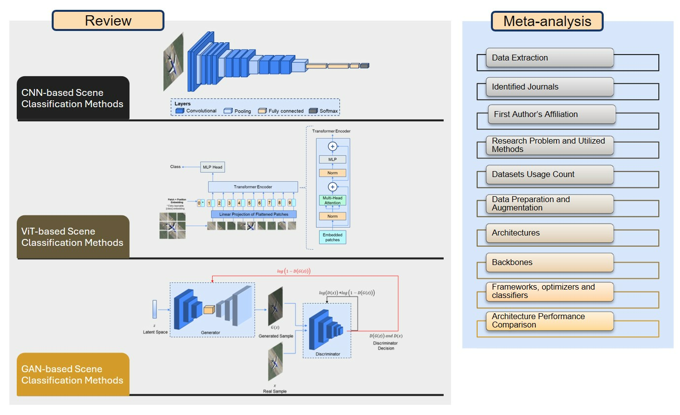
:Remote sensing image scene classification with deep learning (DL) is a rapidly growing field that has gained significant attention in the past few years. While previous review papers in this domain have been confined to 2020, an up-to-date review to show the progression of research extending into the present phase is lacking. In this review, we explore the recent articles, providing a thorough classification of approaches into three main categories: Convolutional Neural Network (CNN)-based, Vision Transformer (ViT)-based, and Generative Adversarial Network (GAN)-based architectures. Notably, within the CNN-based category, we further refine the classification based on specific methodologies and techniques employed. In addition, a novel and rigorous meta-analysis is performed to synthesize and analyze the findings from 50 peer-reviewed journal articles to provide valuable insights in this domain, surpassing the scope of existing review articles. Our meta-analysis shows that the most adopted remote sensing scene datasets are AID (41 articles) and NWPU-RESISC45 (40). A notable paradigm shift is seen towards the use of transformer-based models (6) starting from 2021. Furthermore, we critically discuss the findings from the review and meta-analysis, identifying challenges and future opportunities for improvement in this domain. Our up-to-date study serves as an invaluable resource for researchers seeking to contribute to this growing area of research.

1. Introduction
The advancement in Earth observation technology has led to the availability of very high-resolution (VHR) images of the Earth’s surface. With the development of VHR images, it is possible to accurately identify and classify land use and land cover (LULC) [1], and the demands for such tasks are high. Scene classification in remote sensing images aims to categorize image scenes automatically into relevant classes like residential areas, cultivation land, forests, etc. [2], drawing considerable attention. In recent years, the application of scene classification in VHR satellite images is evident in disaster detection [3], land use [4,5,6,7,8,9], and urban planning [10]. The implementation of deep learning (DL) for scene classification is an emerging tendency in a current scenario, with an effort to achieve maximum accuracy. A review and meta-analysis of these defacto methods is valuable to the research community, but is either lacking or not up-to-date. To this end, we explore DL methods on satellite images for scene classification.
In the early days of remote sensing, the spatial resolution of images was relatively low, resulting in the pixel size equivalent to the object of interest [11]. As a consequence, the studies on remote sensing classification were based on pixel-level [11,12,13]. Subsequently, the increment in spatial resolution reoriented the research to remote sensing classification on the object-level, which produced more enhanced classification than per-pixel analysis [14]. This approach dominated the remote sensing classification domain for decades, including [15,16,17,18,19,20]. However, the perpetual growth of remote sensing images facilitates capturing distinct object classes, rendering traditional pixel-level and object-level methods inadequate for accurate image classification. In such a scenario, scene-level classification became crucial to interpret the global contents of remote sensing images [21]. Thus, numerous experiments can be observed in scene-label analysis over the past few years [22,23,24,25,26]. Figure 1 illustrates the progression of classification approaches from pixel-level to object-level and finally to scene-level.
The preliminary methods for remote sensing scene classification were predominantly relying on low-level features such as texture, color, gradient, and shape. Hand-crafted features like Scale-Invariant Feature Transform (SIFT), Gabor filters, local binary pattern (LBP), color histogram (CH), gray level co-occurrence matrix (GLCM), and histogram of oriented gradients (HOG) were designed to capture specific patterns or information from the low-level features [7,27,28,29,30]. These features are crafted by domain experts and are not learned automatically from data. The methods utilized on low-level features only rely on uniform texture and can not perform on complex scenes. On the other hand, methods on mid-level features extract more complex patterns with clustering, grouping, or segmentation [31,32]. The idea is to acquire local attributes from small regions or patches within an image and encode these local attributes to retrieve the intricate and detailed pattern [33]. The bag-of-visual-words (BoVW) model is a widely used mid-level approach for scene classification in the remote sensing field [34,35,36]. However, the limited representation capability of mid-level approaches has hindered breakthroughs in remote sensing image scene classification.
In recent times, DL models emerged as a solution to address the aforementioned limitations in low-level and mid-level methods. DL architectures implement a range of techniques, including Convolutional Neural Networks (CNNs) [37,38], Vision Transformers (ViT), and Generative Adversarial Networks (GANs), to learn discriminative features for effective feature extraction. For scene classification, the available datasets are grouped into diverse scenes. The DL architectures are either trained on these datasets to obtain the predicted scene class [39], or pretrained DL models are used to obtain derived classes from the same scene classes [40,41], depending upon the application. In the context of remote sensing scene classification, the experiments are mainly focused on achieving optimal scene prediction by implementing DL architectures. CNN architectures like Residual Network (ResNet) [42], AlexNet [43], GoogleNet [44], etc., are commonly used for remote sensing scene classification. Operations like fine-tuning [45], adding low-level and mid-level feature descriptors like LBP [46], BovW [47], etc., and developing novel architectures [33,48] are performed to obtain nearly ideal scene classification results. Furthermore, ViTs and GANs are also used to advance research and applications in this field.
In this paper, a meta-analysis is performed from peer-reviewed research articles that utilized DL-based methods for remote sensing image scene classification. To the best of our knowledge, this meta-analysis is the first of its kind to focus on DL methods in this domain. There are few review papers that evaluate datasets and DL methods [21,49] or include them as a part of a review article [50]. However, these studies provide an overview of experiments performed on DL-based remote sensing scene classification limited to 2020. Therefore, we review this domain as a significant amount of improvement is expected, along with meta-analysis as a novel approach.
The necessity of this research is emphasized by its significance in the domain of remote sensing scene classification using DL. Within this study, we address various insights extracted from this research, including the role of a diverse array of datasets, the notable disparity in accuracy between self-supervised and supervised methods, and the dominance of pretrained CNNs. However, the most crucial revelation is the identification of paradigm shifts that hold transformative implications in this field. This study not only contributes to the current understanding of remote sensing scene classification, but also paves the way for future advancements. These encompass the development of expansive annotated datasets, the further exploration of local–global feature representations within images, the refinement of self-supervised learning techniques to compete with supervised learning, and the pursuit of innovative approaches.
The major contributions of this article are listed below:
- We present an up-to-date review offering insights into remote sensing scene datasets and DL feature extraction methods, encompassing CNN-based, ViT-based and GAN-based approaches, through a comprehensive examination of relevant studies.
- We conduct a novel meta-analysis of 50 peer-reviewed articles in the DL-driven remote sensing scene classification domain. We pinpoint the critical problems and recognize emerging trends and paradigm shifts in this field.
- We identify and discuss key challenges in this domain while also providing valuable insights into future research directions.
2. Understanding Remote Sensing Image Scene and Deep Learning Feature Extraction
2.1. High-Resolution Scene Classification Datasets
Multiple VHR remote sensing datasets are available for scene classification. The UC Merced Land Use Dataset (UC-Merced or UCM) [51] is a popular dataset obtained from the United States Geological Survey (USGS) National Map Urban Area Imagery collection covering US regions. Some of the classes belonging to this dataset are airplanes, buildings, forests, rivers, agriculture, beach, etc., depicted in Figure 2. The Aerial Image Dataset (AID) [23] is another dataset acquired from Google Earth Imagery with a higher number of images and classes than the UCM dataset. Table 1 lists some widely used datasets for scene recognition in the remote sensing domain. Some of the scene classes are common in multiple datasets. For instance, the “forest” class is included in UCM, WHU-RS19 [52], RSSCN7 [53], and NWPU-RESISC45 [49] datasets. However, there are variations in scene classes among different datasets. In addition, the number of images and their size and resolution of scene datasets varies in respective datasets. Thus, the selection of the dataset depends on the research objectives. Cheng et al. [49] proposed a novel large-scale dataset NWPU-RESISC45 with rich image variations and high within-class diversity and between-class similarity, addressing the problem of small-scale datasets, lack of variations, and diversity. Miao et al. [54] merged UCM, NWPU-RESISC45, and AID datasets to prepare a larger remote-sensing scene dataset for semi-supervised scene classification and attained a similar performance to the state-of-the-art methods. In these VHR datasets, multiple DL architectures have been conducted to obtain optimal accuracy.
2.2. CNN-Based Scene Classification Methods
CNNs [60] effectively extract meaningful features from images by utilizing convolutional kernels and hierarchical layers. A typical CNN architecture includes a convolutional layer, pooling layer, Rectified Linear Unit (ReLU) activation layer, and fully connected (FC) layer [61] as shown in Figure 3. The mathematical formula for the output of each filter in a 2D convolutional layer is provided in Equation (1).
where represents the activation function, is the weight associated with the connection between input feature map m and output feature map n, and denotes the bias term associated with output feature map n. The convolution layers learn features from input images, followed by the pooling layer, which reduces computational complexity while retaining multi-scale information. The ReLU activation function introduces non-linearity to the network, allowing for the modeling of complex relationships and enhancing the network’s ability to learn discriminative features. The successive use of convolutional and pooling layers allows the network to learn increasingly complex and abstract features at different scales. The first few initial layers capture low-level features such as edges and textures, while deeper layers learn high-level features and global structures [62]. The FC layers serve as a means of mapping the learned features to the final output space, enabling the network to make predictions based on the extracted information. In a basic CNN structure, the output of an FC layer is fed into either a softmax or a sigmoid activation function for classification tasks. However, the majority of parameters are occupied by an FC layer, increasing the possibility of overfitting. Dropout is implemented to counter this problem [63]. To minimize loss and improve the model’s performance, several optimizers like Adam [64] and stochastic gradient descent (SGD) [65] are prevalent in research.
Multiple approaches have been explored to optimize the feature extraction process for accurate remote sensing scene classification using CNNs. They are sub-divided into two categories: pretrained CNNs and CNNs trained from scratch.
2.2.1. Pretrained CNNs for Feature Extraction
Collecting and annotating data for larger remote sensing scene datasets increases costs and is a laborious task. To address the scarcity of data in the remote sensing domain, researchers often utilize terrestrial image datasets such as ImageNet [66] and PlacesCNN [67], which contain a large number of diverse images from various categories. Wang et al. [68] described the local similarity between remote sensing scene image and natural image scenes. By leveraging pretrained models trained on these datasets, the CNN algorithms can benefit from the learned features and generalize well to remote sensing tasks with limited labeled data. This process is illustrated in Figure 4, showcasing the role of pretrained CNNs.
In 2015, Penatti et al. [30] introduced pretrained CNN on ImageNet into remote sensing scene classification, discovering better classification results for the UCM dataset than low-level descriptors. In a diverse large-scale dataset named NWPU-RESISC45, three popular pretrained CNNs: AlexNet [63], VGG-16 [69] and GoogLeNet [70], improved the performance by 30% minimum compared to handcrafted and unsupervised feature learning methods [49]. NWPU-RESISC45 dataset is ambiguous due to high intra-class diversity and inter-class similarity. Sen et al. [71] adopted a hierarchical approach to mitigate the misclassification. Their method is divided into two levels: (i) all 45 classes are rearranged into 5 main classes (Transportation, Water Areas, Buildings, Constructed Lands, Natural Lands), and (ii) the 45 sub-levels are trained in each class. DenseNet-121 [72] pretrained on ImageNet is used as a feature extractor in both levels. Al et al. [73] combined four scene datasets, namely UCM, AID, NPWU, and PatternNet, to construct a heterogeneous scene dataset. For suitability, the 12 shared classes are filtered to utilize an MB-Net architecture, which is based on pretrained ResNet-50 [74]. MB-Net is designed to capture collective knowledge from three labeled source datasets and perform scene classification on a remaining unlabeled target dataset. Shawky et al. [75] brought a data augmentation strategy for CNN-MLP architecture with Xception [76] as a feature extractor. Sun et al. [77] obtained multi-scale ground objects using multi-level convolutional pyramid semantic fusion (MCPSF) architecture and differentiated intricate scenes consisting of diverse ground objects.
Yu et al. [78] introduced a feature fusion strategy in which CNNs are utilized to extract features from both the original image and a processed image obtained through saliency detection. The extracted features from these two sources are then fused together to produce more discriminative features. Ye et al. [79] proposed parallel multi-stage (PMS) architecture based on the GoogleNet backbone to learn features individually from three hierarchical levels: low-, middle-, and high-level, prior to fusion. Dong et al. [80] integrated a Deep Convolutional Neural Network (DCNN) with Broad Learning System (BLS) [81] for the first time in the remote sensing scene classification domain to extract shallow features and named it FDPResNet. The DCNN implemented ResNet-101 pretrained on ImageNet as a backbone on both shallow and deep features and further fused and passed to the BLS system for classification. CNN architectures for remote sensing scene classification vary in design with the incorporation of additional techniques and methodologies. However, the widely employed approaches include LBP-based, fine-tuning, parameter reduction, and attention mechanism methods.
LBP-based pretrained CNNs: LBP is a widely used robust low-level descriptor for recognizing textures [82]. In 2018, Anwer et al. [46] proposed Tex-Net architecture, which combined an original RGB image with a texture-coded mapped LBP image. The late fusion strategy (Tex-Net-LF) performed better than early fusion (Tex-Net-EF). Later, Yu et al. [83], who previously introduced the two-stream deep fusion framework [78], adopted the same concept to integrate the LBP-coded image as a replacement for the processed image obtained through saliency detection. However, they conducted a combination of previously proposed and new experiments using the LBP-coded mapped image and fused the features together. Huang et al. [84] stated that two-stream architectures solely focus on RGB image stream and overlook texture-containing images. Therefore, CTFCNN architecture based on pretrained CaffeNet [85] extracted three kinds of features: (i) convolutional features from multiple layers, wherein each layer improved bag-of-visual words (iBoVW) method represented discriminating information, (ii) FC features, and (iii) LBP-based FC features. Compared to traditional BoVW [35], the iBoVW coding method achieved rational representation.
Fine-tuned pretrained CNNs: Cheng et al. [49] not only used pretrained CNNs for feature extraction from the NWPU-RESISC45 dataset, they further fine-tuned the increasing learning rate in the last layer to gain better classification results. For the same dataset, Yang et al. [86] fine-tuned parameters utilized on three CNN models: VGG-16 and DenseNet-161 pretrained on ImageNet used as deep-learning classifier training, and feature pyramid network (FPN) [87] pretrained on Microsoft Coco (Common Objects in Context) [88] for deep-learning detector training. The combination of DenseNet+FPN exhibited exceptional performance. Zhang et al. [33] used the hit and trial technique to set the hyperparameters to achieve better accuracy. Petrovska et al. [89] implemented linear learning rate decay, which decreases the learning rate over time, and cyclical learning rates [90]. The improved accuracy utilizing fine-tuning on pretrained CNNs validates the statement made by Castelluccio et al. [91] in 2015.
Parameters reduction: CNN architectures exhibit a substantial amount of parameters, such as VGG-16, which comprises approximately 138 million parameters [92]. The large number of parameters is one of the factors for over-fitting [93,94]. Zhang et al. [95] utilized DenseNet, which is known for its parameter efficiency, with around 7 million parameters. Yu et al. [96] integrated light-weighted CNN MobileNet-v2 [97] with feature fusion bilinear model [98] and termed the architecture as BiMobileNet. BiMobileNet featured a parameter count of 0.86 million, which is six, eleven, and eighty-five times lower than the parameter numbers reported in [83], [45] and [99], respectively, while achieving better accuracy.
Attention mechanism: In the process of extracting features from entire images, it is essential to consider that images contain various objects and features. Therefore, selectively focusing on critical parts and disregarding irrelevant ones becomes crucial. Zhao et al. [100] added a channel-spatial attention [101] module (CBAM) following each residual dense block (RDB) based on DenseNet-101 backbone pretrained on ImageNet. CBAM helps to learn meaningful features in both channel and spatial dimensions [102]. Ji et al. [103] proposed an attention network based on the VGG-VD16 network that localizes discriminative areas in three different scales. The multiscale images are fed to sub-network CNN architectures and further fused for classification. Zhang et al. [104] introduced a multiscale attention network (MSA-Network), where the backbone is ResNet. After each residual block, the multiscale module is integrated to extract multiscale features. The channel and position attention (CPA) module is added after the last multiscale module to extract discriminative regions. Shen et al. [105] incorporated two models, namely ResNet-50 and DenseNet-121, to fulfill the insufficiency of single CNN models. Both models captured low, middle, and high-level features and combined them with a grouping-attention-fusion strategy. Guo et al. [106] proposed a multi-view feature learning network (MVFL) divided into three branches: (i) channel-spatial attention to localize discriminative areas, (ii) triplet metric branch, and (iii) center metric branch to increase interclass distance and decrease intraclass distance. Zhao et al. [107] designed an enhanced attention module (EAM) to enhance the ability to understand more discriminative features. In EAM, two depthwise dilated convolution branches are utilized, each branch having different dilated rates. Dilated convolutions enhance the receptive fields without escalating the parameter count. They effectively capture multiscale contextual information and improve the network’s capacity to learn features. The two branches are merged with depthwise convolutions to decrease the dimensionality. Hu et al. [108] introduced a multilevel inheritance network (MINet), where FPN based on ResNet-50 is adopted to acquire multilayer features. Subsequently, an attention mechanism is employed to augment the expressive capacity of features at each level. For the fusion of features, the feature weights across different levels are computed by leveraging the SENet [109] approach.
2.2.2. CNNs Trained from Scratch
Pretrained CNNs are typically trained on large-scale datasets such as ImageNet, which are not adaptable to the specific characteristics of the target dataset. Modifying pretrained CNNs is inconvenient due to the complexity and compatibility of CNNs. Although pretrained CNNs attained outstanding classification results, Zhang et al. [110] addressed complexity in pretrained CNNs due to the extensive parameter size and implemented a light-weighted CNN MobileNet-v2 with dilated convolution and channel attention. He et al. [111] introduced a skip-connected covariance (SCCov) network, where a skip connection is added along with covariance pooling. The SCCov architecture reduced the parameter number with better scene classification. Zhang et al. [112] proposed a gradient-boosting random convolutional network to assemble various non-pretrained deep neural networks (DNNs). A simplified representation of CNN architectures trained from scratch is illustrated in Figure 3. This CNN is solely based on a dataset to be trained without the involvement of pretrained CNN on a specific dataset.
2.3. Vision Transformer-Based Scene Classification Methods
The ViT [113] model can perform image feature extraction without relying on convolutional layers. This model utilizes a transformer architecture [114], initially introduced for natural language processing. In ViT, an input image undergoes partitioning into fixed-size patches, and each patch is then transformed into a continuous vector through a process known as linear embedding. Moreover, position embeddings are added to the patch embeddings to retain positional information. Subsequently, a set of sequential patches (Equation (2)) are fed into the transformer encoder, which consists of alternating layers of Multi-head Self-Attention (MSA) [114] (Equation (3)) and multi-layer perceptron (MLP) (Equation (4)). Layernorm (LN) [115] is implemented prior to both MSA and MLP to reduce training time and stabilize the training process. Residual connections are applied after every layer to improve the performance. The MLP has two layers with a Gaussian Error Linear Unit (GELU) [116] activation function. In the final layer of the encoder, the first element of the sequence is passed to an external head classifier for prediction (Equation (5)). Figure 5 illustrates the ViT architecture for remote sensing scene classification.
where represents the embedding for the class token. denotes the embeddings of different patches flattened from the original images, concatenated with . is a matrix representing patch embeddings where P is patch size, C is the number of channels, and D is the embedding dimension. Positional embedding is added to patches, accounting for positions (including class token), each in a D-dimensional space.
where is the output of the MSA layer, applied after LN to the -th layer’s output (i.e., ), incorporating a residual connection. L represents the total number of layers in the transformer.
where is the output of the MLP layer, applied after LN to the from the -th layer, incorporating a residual connection. L represents the total number of layers in the transformer.
ViT performs exceptionally well in capturing contextual features. Bazi et al. [117] introduced ViT for remote sensing scene classification and obtained a promising result compared to state-of-the-art CNN-based scene classification methods. Their method involves data augmentation strategies to improve classification accuracy. Furthermore, the network is compressed by pruning to reduce the model size. Bashmal et al. [118] utilized a data-efficient image transformer (DeiT), which is trained by knowledge distillation with a smaller dataset and showed potential results. Bi et al. [119] used the combination of ViT and supervised contrastive learning (CL) [120], named ViT-CL, to increase the robustness of the model by learning more discriminative features. ViT performs exceptionally well in capturing contextual features. However, they face limitations in learning local information. Moreover, their computational complexity is significantly high [121]. Peng et al. [122] addressed the challenge and introduced a local–global interactive ViT (LG-ViT). In LG-ViT architecture, images are partitioned to learn features in two different scales: small and large. ViT blocks learn from both scales to handle the problem of scale variation. In addition, a global-view network is implemented to learn global features from a whole image. The features obtained from the global-view network are embedded with local representation branches, which enhance local–global feature interaction.
CNNs excel at preserving local information but lack the ability to comprehensively capture global contextual features. ViTs are well-suited to learn long-range contextual relations. The hybrid approach of using CNNs and transformers leverages the strengths of both architectures to improve classification performance. Xu et al. [121] integrated ViT and CNN to harness the strength of CNN. In their study, ViT is used to extract rich contextual information, which is transferred to the ResNet-18 architecture. Tang et al. [123] proposed an efficient multiscale transformer and cross-level attention learning (EMTCAL), which also combines CNN with a transformer to extract maximum information. They employed ResNet-34 as a feature extractor in the CNN model. Zhang et al. [124] proposed a remote sensing transformer (TRS) to capture the global context of the image. TRS combines self-attention with ResNet through the Multi-Head Self-Attention layer (MHSA), replacing the conventional 3 × 3 spatial convolutions in the bottleneck. Additionally, the approach incorporates multiple pure transformer encoders, leveraging attention mechanisms to enhance the learning of representations. Wang et al. [125] utilized pretrained Swin Transformer [126] to capture features at multilayer followed by patch merging to concatenate the patches (except in the last block), with these two elements forming the Swin Transformer Block (STB). The multilevel features obtained from STB are eventually merged with the inspired technique [87], then further compressed using convolutions within the adaptive feature compression module because of redundancy in multiple features. Guo et al. [127] integrated Channel-Spatial Attention (CSA) into the ViT [113] and termed the architecture Channel-Spatial Attention Transformers (CSAT). The combined CSAT model accurately acquires and preserves both local and global knowledge.
2.4. GAN-Based Scene Classification Methods
Supervised learning methods effectively perform remote sensing scene classification. However, due to limited labeled scene images, Miao et al. merged UCM, NWPU-RESISC45, and AID datasets to create larger remote-sensing scene datasets [54]. Annotating samples manually for labeling scenes is laborious and expensive. GAN [128] can extract meaningful information using unlabeled data. GAN is centered around two models: the generator and the discriminator, illustrated in Figure 6. The generator is trained to create synthetic data that resemble real data, aiming to deceive the discriminator. On the other hand, the discriminator is trained to distinguish between the generated (fake) data and the real data [129]. The overall objective of GAN is to achieve a competitive interplay between these two models, driving the generator to produce increasingly realistic data samples while the discriminator becomes better at detecting the generated data. In Equation (6), the value function describes the training process of GAN as a minimax game.
where the input from the latent space z is provided to the generator G to generate synthetic image G(z). G(z) is further fed to the discriminator D, alongside the real image x. The discriminator predicts both samples as synthetic (0) or real (1) based on its judgment. This process optimizes G and D through a dynamic interplay. G trains to minimize , driving it to create synthetic images that resemble real ones. Simultaneously, D trains to maximize + , refining its ability to distinguish real from synthetic samples.
Lin et al. [130] acknowledged the unavailability of sufficient labeled data for remote sensing scene classification, which led them to introduce multiple-layer feature-matching generative adversarial networks (MARTA GANs). MARTA GANs fused mid-level features with global features for learning better representations by a descriptor. Xu et al. [131] replaced ReLU with scaled exponential linear units (SELU) [132] activation, enhancing GAN’s ability to produce high-quality images. Ma et al. [133] addressed that samples generated by GAN are solely used for self-training and introduced a new approach, SiftingGAN, to generate a significant number of authentic labeled samples. Wei et al. [134] introduced multilayer feature fusion Wasserstein GAN (MF-WGANs), where the multi-feature fusion layer is subsequent to the discriminator to learn mid-level and high-level feature information.
In unsupervised learning methods, labeled image scenes remain unexplored. However, leveraging annotations can significantly enhance classification capabilities. Therefore, Yan et al. [135] incorporated semi-supervised learning into GAN, aiming to exploit the benefits of labeled images and enhance classification performance. Miao et al. [54] introduced a semi-supervised representation consistency Siamese network (SS-RCSN), which incorporates Involution-GAN for unsupervised feature learning and a Siamese network to measure the similarity between labeled and unlabeled data in a high-dimensional space. Additionally, representation consistency loss in the Siamese network aids in minimizing the disparities between labeled and unlabeled data.
3. Meta-Analysis
In this section, a meta-analysis is conducted to synthesize and analyze the findings from multiple studies in the domain of DL for remote sensing scene classification. We begin by extracting relevant papers from a collection of peer-reviewed articles in the Scopus database, followed by a meticulous filtering process. Within the selected articles, the meta-analysis encompasses various aspects, including (i) addressing the research problems and utilizing corresponding research techniques, (ii) examining data usage frequency, (iii) exploring data preparation and augmentation methods, (iv) collecting information on the architectures, backbones, frameworks, optimizers, and classifiers involved during training, and (v) comparing architectures used in these articles. From this meta-analysis, we aim to provide valuable insights into the advancements and trends in DL methods for remote sensing scene classification.
3.1. Data Extraction
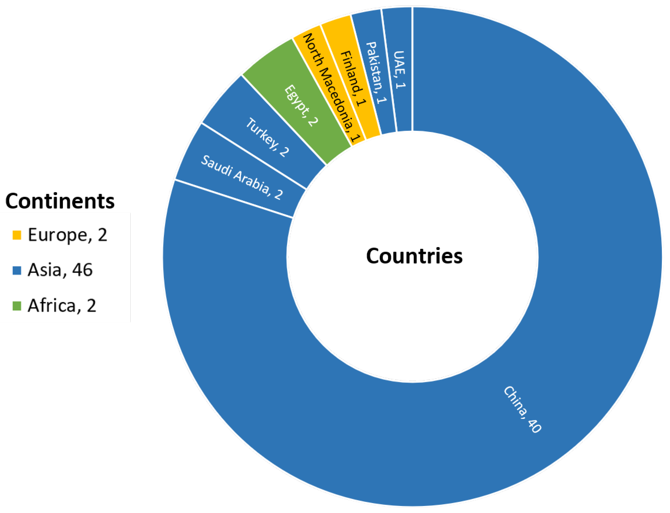
Firstly, articles regarding remote sensing scene classification were identified with a search conducted in the Scopus database. The search query involved article title/keywords/abstracts with terms: [“scene classification”] AND [“aerial image dataset” OR “nwpu-resisc45” OR “whu-rs19” OR “uc merced land used dataset”] AND [[“remote sensing”] OR [“satellite image”]] (search date: 2 May 2023). While using [“scene classification”] AND [[“remote sensing”] OR [“satellite image”]] for the query, Scopus resulted in an irrelevant list of articles without scene-labeled datasets. In addition, adding [“aerial image”] to the following query, [“aerial image”] only referred to the AID dataset in many cases, which restricts the research paper to AID dataset-related papers. Thus, specific datasets were mentioned as they are commonly used, and there is a high probability of utilizing at least one of them in research articles. The articles were limited to journal papers and review papers to exclude conference papers, resulting in 148 peer-reviewed articles. However, our bibliographical analysis is mainly focused on DL-implemented methods, comprehensive utilization of the entire dataset, free from language barriers, and accessible journal papers (including foreign access restriction). As a result, 50 articles were selected for meta-analysis, which attempted to fulfill the interpretation of DL for the remote sensing scene classification context. Figure 7 illustrates the respective journal names along with their counts for the filtered peer-reviewed articles. In Figure 8, a visualization is presented, showcasing the countries and continents associated with the affiliations of the first authors.
3.2. Research Problem and Utilized Research Techniques
The filtered 50 articles target specific research problems, as depicted in Table 2, with a shared objective of enhancing remote sensing scene classification accuracy. Among the articles, 11 specifically focused on capturing more discriminative regions through the fusion of processed images in [75,78,83], multilayer fusion in [79,80,125,136,137], FC replaced by CapsNet [138] in [33,139], and pairwise comparison in [140]. To focus on key regions, attention mechanism is introduced in [100,103,104,106,107], while the use of classifier-detector is introduced in [86] and multiple instance learning (MIL) [141] in [142]. Additionally, learning local and global information in conjunction is primarily based on transformer-based networks [122,124,127,143,144], while the utilization of the dual-branch network is explored in [145]. Meanwhile, lightweight CNNs are used in [10,96] and DenseNet in [95]. For reducing the effect of high intra-class diversity and high inter-class similarity in the dataset, metric branches [106] and re-organized classes in a two-layer hierarchy [71] are implemented. The utilized techniques on respective research problems are shown in the same Table 2. It is also noticed that [83,106] aims to solve multiple research problems.
3.3. Dataset Usage Frequency
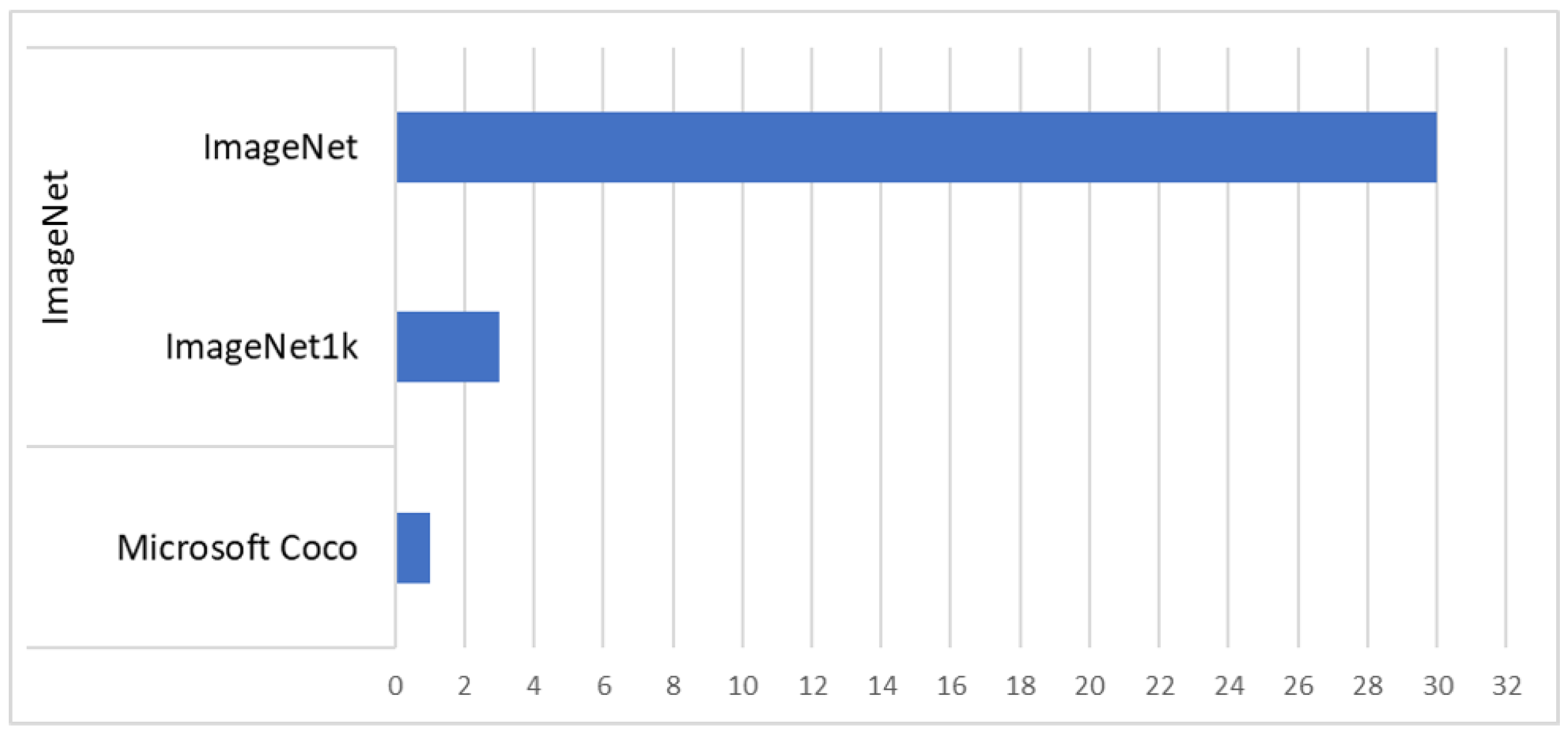
In common, multiple datasets are used within the same research papers across a set of 50 research articles. Figure 9 illustrates the dataset number used in these papers. The analysis reveals that the AID dataset is the most frequently used, with a count of 41, followed closely by NWPU-RESISC45, with a count of 40. Indian Pines [160] is the only dataset containing hyperspectral images. UCM [51], AID [23], WHU-RS19 [52], NWPU-RESISC45 [49], RSSCN7 [53], PatternNet [55], OPTIMAL-31 [56], KSA [59], SIRI-WHU [57] and RSI-CB [58] contains orginal RGB labeled images. Meanwhile, Corel-1K and Corel-1.5K [161] are terrestrial image datasets used for analysis along with other remote sensing scene datasets in [148]. The links to these remote sensing scene datasets are provided in Appendix A. For pretrained models, the backbones are pretrained on existing datasets. This means that the initial training of the model is performed on large-scale datasets such as ImageNet (33 articles) and COCO (1 article), as shown in Figure 10. The datasets utilized for each study are documented in Appendix B.
3.4. Data Preparation and Augmentation
Data preparation involves resizing the images to match the required input size. Among the surveyed articles, the majority (17 articles) employ an image size of 224 × 224 pixels as the standard for input in their architecture. However, it is worth noting that a small subset of articles (3 articles) demonstrate the adaptability of architectures by accepting images of varying sizes. This highlights the flexibility of certain DL approaches in accommodating different image dimensions. Figure 11 displays the frequency distribution of image sizes employed in the articles included in the meta-analysis.
The data augmentation practice is applied with the objective of expanding the dataset [162]. Notably, a total of 20 articles in this study involve the use of data augmentation as a method to enhance their classification accuracy. However, two articles explicitly state that they did not implement any data augmentation technique in their study. Figure 12 shows the distribution of data augmentation techniques implemented among these articles. The most prevalent technique utilized is rotation, with or without a random angle, implemented in 15 articles. Following close behind is the technique of either horizontal or vertical flip, which is used in 13 articles. It is observed that many research studies employ a combination of these data augmentation methods, effectively improving their classification accuracy. More details are provided in Appendix B.
3.5. Training Details
The training process of a DL architecture involves various aspects, including the training percentage, the chosen architecture, frameworks, implemented optimizers, and hyperparameters. The training percentage is determined based on the size of the dataset, ensuring an appropriate allocation of data for model training. Table 3 presents the most commonly used training percentages for the frequently employed datasets.
When it comes to selecting architecture, several architectures are frequently utilized in research studies. Among these architectures, GoogleNet is selected six times, indicating its usage in multiple instances. Additionally, other commonly employed architectures include VGG-16, ResNet-50, and CaffeNet. However, it is important to note that researchers also explore and implement novel architectures, showcasing continuous innovation and experimentation within the field of architecture design. Figure 13 provides a visual representation to visually explore the popular DL architectures, excluding the novel ones. Furthermore, in Figure 14, the mapping of all the backbones used in each architecture utilized in our meta-analysis is presented. It is observed that ResNet-50 is the most frequently used backbone, appearing 15 times, followed by VGG-16 (12 times), ResNet-101 (6 times), and CaffeNet (6 times). The DL architectures and backbones used for each study are documented in Appendix B.
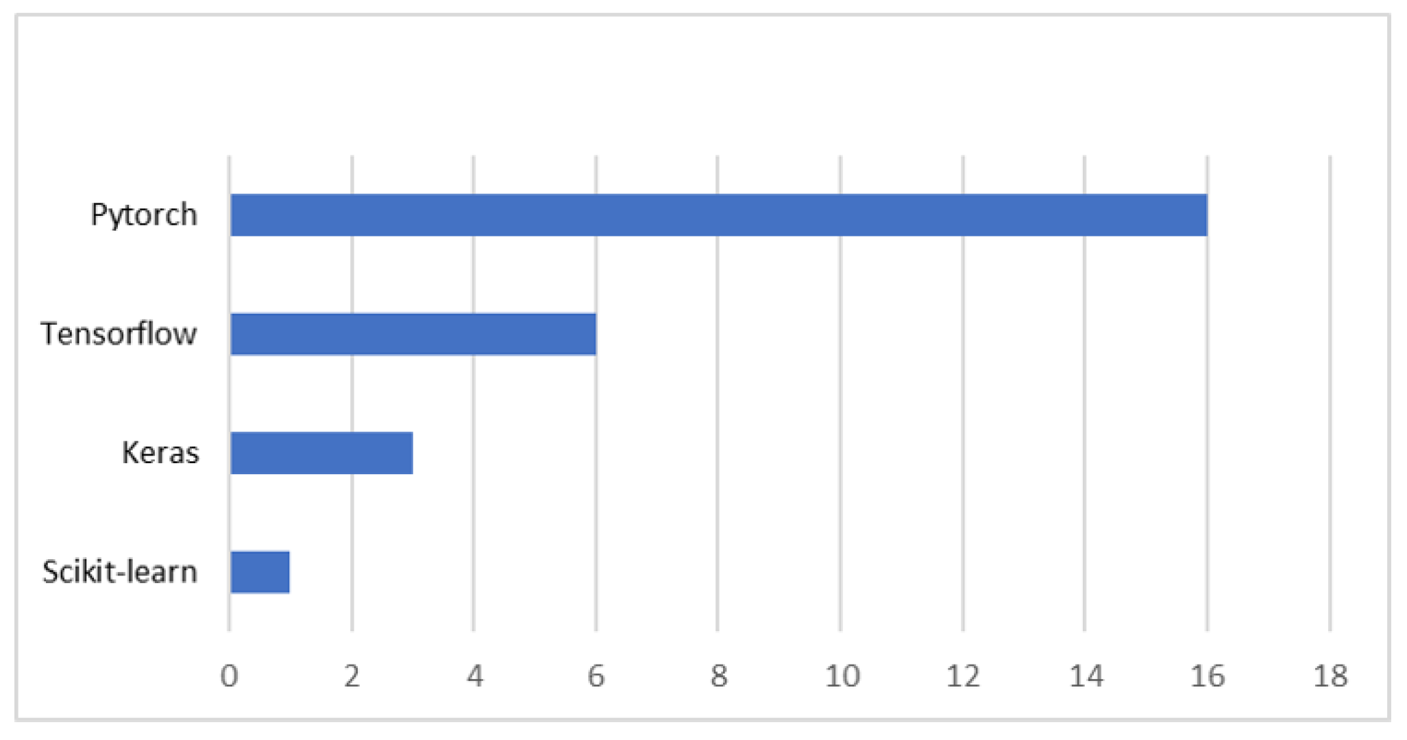
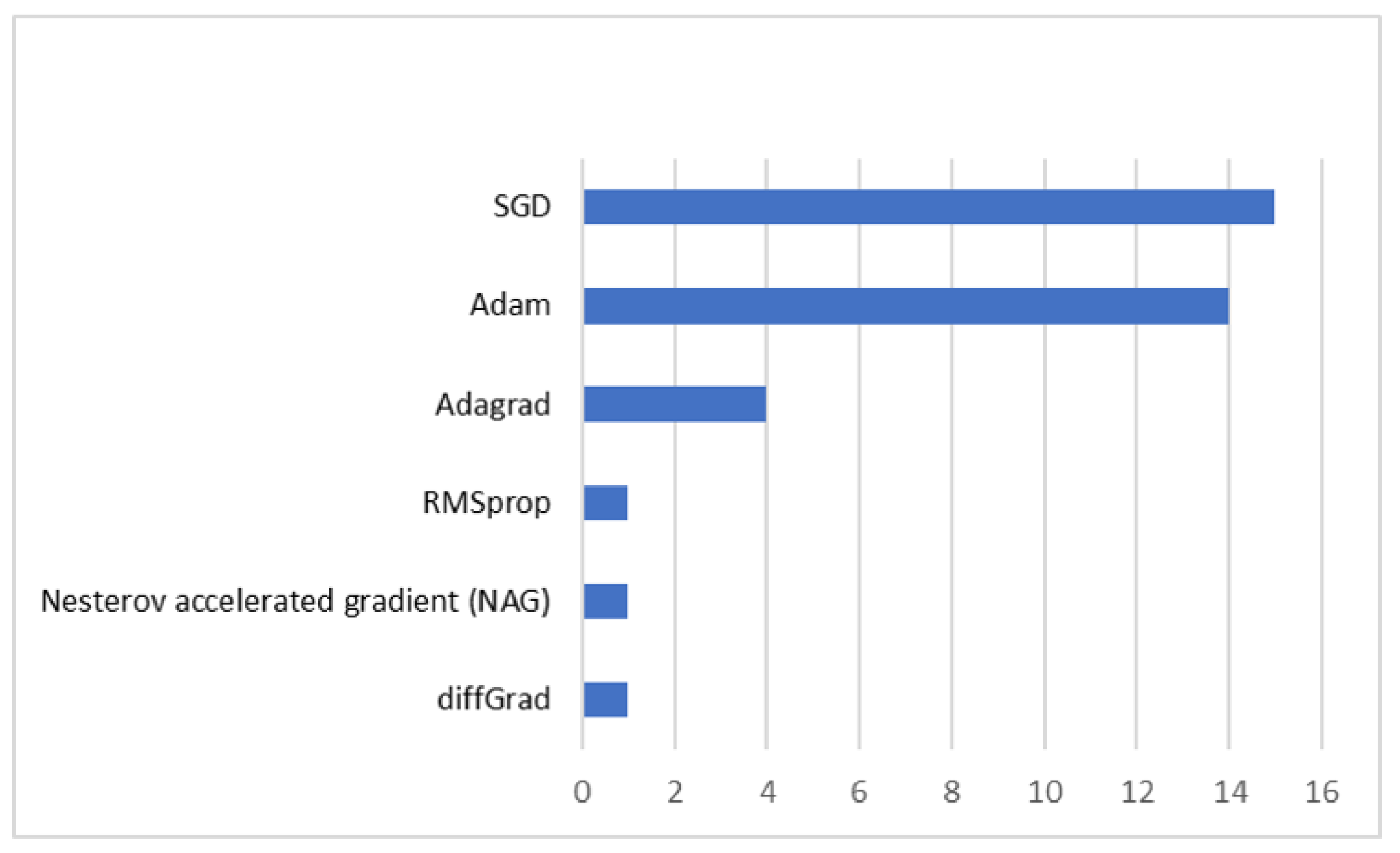
Frameworks in DL architecture for remote sensing scene classification are important for providing a structured platform, flexibility, and efficiency in developing and training DL models. As depicted in Figure 15, PyTorch [163], TensorFlow [164], Keras [165], and scikit-learn [166] are the commonly employed frameworks in this field, with PyTorch being the most frequently used among them. Optimizers are also utilized to adjust the parameters of DL models during training, aiming to minimize the loss function and enhance classification accuracy. The implemented optimizers are Adam, SGD, Adagrad [167], RMSprop [168], Nesterov accelerated gradient (NAG) [169] and diffGrand [170] (see Figure 16). Moreover, among the classifiers used in remote sensing scene classification, support vector machine (SVM) [171] and softmax are the most prevalent, surpassing other classifiers, as depicted in Figure 17. More details are provided in Appendix B.
3.6. Architecture Performance Comparison
The comparison of architectures in this study is centered around the three most commonly used datasets: UCM, AID, and NWPU-RESISC45. All architectures are evaluated using the overall accuracy (OA) metric to facilitate a comprehensive comparison. The expression of OA (in percentage) is presented in Equation (7).
where TP (True Positive) represents the count of correctly classified samples, and Total Samples corresponds to the total number of test images within the dataset. To ensure fairness, the DL architectures trained with specific training rates of 80% for UCM, 50% for AID, and 20% for NWPU-RESISC datasets are selected. Standard deviation values are not considered in the comparison due to their absence in some reviewed papers. Furthermore, some reviewed articles employ multiple architectures or conduct ablation tests to assess the performance of different models. The best-performing architecture is then reviewed and analyzed specifically within the context of these three datasets. Table 4 illustrates the performance of available architectures employed on UCM, AID, and NWPU-RESISIC45.
For the UCM dataset at 80% training data, most architectures achieve over 97% accuracy, except Yan et al. [135], a GAN-based architecture for semi-supervised learning, which achieves 94.05% accuracy. The lowest performing supervised architecture is local and convolutional pyramid-based pooling-stretched (LCPP) [77] model with 97.54% accuracy, which focuses on effectively extracting multiscale feature maps. Notably, the best-performing DL architecture is LG-VIT [122], a transformer-based network that effectively captures both global and local information, achieving 99.93% accuracy. All grains, one scheme AGOS [142] framework also achieves outstanding performance with 99.88% accuracy.
When examining the AID dataset at a 50% training ratio, it is evident that CBAM+RDN [100] with an attention mechanism achieves the highest accuracy among the architectures with 99.08%. TRS [124], a transformer-based network, follows closely as the second-best performer with an accuracy of 98.48%. On the other hand, MF-WGAN [134], an unsupervised learning model, achieves the lowest accuracy (80.35%). LCPP is the lowest-performing supervised architecture with 93.12% classification accuracy.
In the case of the NWPU-RESISC45 dataset trained at 20% data, the Xception-based CNN-MLP [75] architecture achieves the highest accuracy of 97.40%. The Xception-based method, proposed by Shawky et al. [150], which fused the VHR image and saliency map obtained using the saliency algorithm [172], is the second high-performing architecture. Conversely, the fusion of the original VHR image and the processed VHR image with saliency detection using VGG-Net-16 [78] and CaffeNet [78] obtains the lowest accuracy of 83.02% and 83.16%, respectively. Another two-stream architecture that fuses the original image with the mapped LBP image and the original image with the processed image through saliency detection achieves only 87.01% classification accuracy. Table 5 shows the minimum, maximum, and average accuracy values obtained from DL architectures under the same condition as described in Table 4. This information is useful for discussing the importance of the dataset and its utilization in the context of remote sensing scene classification.
4. Discussion
4.1. DL’s Performance Dependency on Datasets
From Table 1, we can observe that the total number of images in UCM, AID, and NWPU-RESISC45 are 2100, 10,000, and 31,500, respectively. The allocation of data for training is determined based on the dataset size and is consistently followed across most of the research articles. This dataset dependency plays a crucial role in the performance of DL methods, as seen in Table 5, where we observe better performance in the UCM dataset. In addition, UCM has a lower number of classes compared to AID and NWPU-RESISC45, indicating higher intra-class diversity and potentially higher inter-class similarity in AID and NWPU-RESISC45. The increment in the training ratio in datasets can boost the performance of DL architectures. Refs. [103,104,105,106,107] used multiple training ratios, commonly used ratios illustrated in Table 3, where the highest training ratio obtained better classification accuracy.
4.2. Low Accuracy in GAN-Based Methods
Unsupervised learning models operate without the need for labeled datasets, whereas semi-supervised learning models do not fully exploit the labeled dataset as they leverage the unlabeled data. In Table 4, it is evident that the unsupervised model MF-WGAN [134] achieved the lowest accuracy of 80.35% on the AID dataset. The difference in accuracy between the unsupervised model and the lowest-performing supervised model is approximately 13%. However, when the training ratio is increased to 80%, the accuracy boosts up to 92.45%. It can be observed that the accuracy of unsupervised learning models increases with a higher training ratio. The same architecture in the NWPU-RESISC45 dataset achieved a lower accuracy of 79.49% accuracy at an 80% training ratio, outperforming another unsupervised architecture named MARTA-GANs [130], which achieved 75.43% accuracy. However, the accuracy of MF-WGAN fell short compared to supervised learning models.
The semi-supervised model based on Marta-GAN [135] achieved the lowest accuracy of 94.05% on the UCM dataset at an 80% training ratio, which is approximately 3.5% lower than the lowest performing supervised learning model of our meta-analysis. The performance of this architecture is also suboptimal on the AID dataset, achieving an accuracy of 83.12% at a 20% training ratio. However, when the training ratio is increased to 80%, the performance improved significantly to 92.78%. This highlights the importance of a higher training ratio for enhancing the performance of semi-supervised models. When SS-RCSN [54] is trained at a 60% training ratio, the accuracy improved up to 98.10%, 94.25%, and 92.03% for the respective UCM, AID, and NWPU-RESISC45 datasets. However, the performance is still lacking compared to the architectures that fully exploit labeled datasets.
From the classification performance, it is understood that semi-supervised learning models are superior to unsupervised learning models because of the utilization of the labeled dataset. However, the classification performance is still lacking compared to supervised learning models. Increasing the training ratio can boost performance to a certain degree, which is contrary to the desired direction. Despite the limitations, GAN is highly useful for minimizing domain shift problems, which occur due to the difference in training and testing datasets [129].
4.3. Shift of Paradigm in Scene Classification Architectures
From Table 4, it is evident that there has been a notable shift in the research focus over time. In the early phase, there was a strong emphasis on fine-tuned and LBP-based architectures, as well as approaches aimed at reducing parameters. Fine-tuned CNNs [86,89] involved modifications to hyper-parameters to optimize performance, while LBP-based CNNs [46,83,84] utilized LBP mapped images to capture texture information for scene classification. Lightweight CNNs [10,96] prioritize parameter reduction for faster performance. These methods, however, often face challenges in effectively classifying complex scenes due to their reliance on processing the entire image as a whole.
Since 2020, there has been a notable shift in research toward the incorporation of attention mechanisms. This approach has the ability to focus on key features or regions within an image to capture relevant information. During our meta-analysis, attention-based CNNs for remote sensing scene classification [100,103,104,105,106,107,108,143] have demonstrated promising performance. CBAM+RDN [100] obtained the highest accuracy of 99.08% on the AID dataset. The minimum accuracies achieved by these architectures are 98.96%, 96.01%, and 93.49% for UCM, AID, and NWPU-RESISC45 datasets, respectively.
Attention-based methods in CNN architectures typically focus on capturing local dependencies while ignoring global information. In recent years, transformer-based methods have gained a significant amount of attention due to their ability to capture both local and global information. By leveraging self-attention mechanisms, transformers can effectively model long-range dependencies and consider the broader context of the input data. Based on our meta-analysis, LG-ViT [122] emerged as the top-performing architecture on the UCM dataset, while TRS [124] achieved the second-best performance on the AID dataset. Furthermore, in the case of the NWPU-RESISC45 dataset, transformer-based methods outperformed LBP-based and fine-tuned methods. This showcases their superiority in capturing both local and global information for effective scene classification.
4.4. Dependency on Pretrained Models
It is evident from our analysis that supervised architectures generally outperform GAN-based architectures, particularly those that prioritize key features or regions within the input data. However, it is important to note that many of these architectures rely on pretrained models, which can provide valuable pre-existing knowledge and improve the performance of the models. The use of pretrained models allows the architectures to leverage the learned representations from large-scale datasets, leading to better generalization and performance on the target datasets. Our meta-analysis indicates that a significant majority (66%) of the reviewed articles stated that they depend on pretrained architectures. In contrast, only a small percentage (6%) confirmed that they trained their architectures from scratch.
Among the 34 articles that stated the use of pretrained models, it is notable that 33 architectures relied on the ImageNet dataset for pretraining. Out of these, three articles specifically utilized the ImageNet1k, a subset of the ImageNet dataset. Conversely, only one article reported the use of the Microsoft Coco dataset for pretraining their architecture. This demonstrates a significant preference for the ImageNet dataset as a source of pretraining DL architectures due to the larger number of available annotated images. The non-pretrained models are GAN-based architectures [134,135] and deep color fusion VGG-based CNN architecture [157] with low accuracy compared to pretrained DL architectures.
Risojevic et al. [173] questioned the necessity of the ImageNet dataset for pretraining, and discovered that we can still derive advantages. However, the dependency on ImageNet for pretraining can be attributed to the scarcity of labeled scene datasets. Researchers have applied various data augmentation approaches to increase the size of the dataset, as shown in Figure 12 of our analysis. Al et al. [73] combined the labeled images from multiple source domains to learn invariant feature representations. This further emphasizes the ongoing need for larger and more comprehensive scene-labeled datasets in the field of remote sensing scene classification. Other than data augmentation, different optimizers, and classifiers are also used to improve the performance of architecture. From our analysis, SGD and Adam are the most used optimization techniques, while SVM and softmax are commonly used for efficient classification.
4.5. Challenges and Future Opportunities
Based on the insights gained from reviewed papers, it is evident that there is always room for improvement in the accuracies obtained from architectures (see Table 4) used for remote sensing scene classification, despite the success obtained in recent years. Through our investigation, we have identified several areas that are expected to be explored in future research to achieve better classification results.
4.5.1. Requirement of Large Annotated Datasets
From Figure 9, it is seen that AID and NWPU-RESISC45 are the most commonly used datasets in remote sensing scene classification research, primarily due to their larger image repositories. Despite their popularity, these datasets are still limited in numbers, leading to the use of pretrained models, often sourced from ImageNet, for transfer learning purposes. However, transfer learning may not always be the optimal solution as pretrained models might not fully adapt to the target domain’s specific characteristics.
A noteworthy approach presented by Miao et al. [54] involves addressing the data scarcity challenge by merging multiple source datasets, thereby increasing the number of available image samples. However, it is essential to consider that different dataset sources may contain uncommon scene classes and are discarded. Moreover, while data augmentation techniques are widely used to enhance the dataset’s diversity and increase sample size, they may have limitations in fully capturing the complexity and variety of real-world scenes. Therefore, the development of large-scale annotated remote sensing scene datasets with a higher number of classes is very promising.
4.5.2. Preservation of Local-Global Features
By learning local features, the model can focus on key information from specific regions or objects within the image. Meanwhile, extracting global features enables the model to understand the overall context and spatial relationships between different portions within the image. The combination of local-global feature representation captures fine-grained details and overall spatial context and can effectively handle diverse and complex scenes. Transformer-based CNN architectures have the capacity to capture and well-preserve both local and global contextual information, with promising results and increased recognition in remote sensing scene classification [124,144] over the past two years. Therefore, it is expected that there will be exploration and utilization in this domain to a greater extent.
4.5.3. Self-Supervised Learning for Scene Classification
Although fully supervised architectures have superior scene classification performance, the data annotation task is laborious and expensive. Exploring different strategies in GAN-based methods presents an opportunity to improve the accuracy of remote sensing scene classification by leveraging unlabeled datasets. By utilizing these unlabeled datasets, the need for manual annotation is reduced, resulting in significant time and cost savings. The GAN-based approach has been utilized [54,134,135] for self-supervised learning. However, the outcome is not as effective as supervised learning. Therefore, it is valuable to continue exploring and developing non-fully supervised models to enhance the performance of remote sensing scene classification.
4.5.4. Learning with Few Data
To avoid data scarcity in remote sensing scene classification, leveraging limited samples can offer a flexible and cost-efficient solution. Quick learning methods such as one-shot [174] and few-shot [175] learning have been explored with the minimal amount of data for scene classification [176,177,178,179]. These methods aim to mimic the human capability to quickly learn and recognize new concepts or classes with very limited examples. However, the classification accuracy is very low, and they struggle to distinguish the scenes as current approaches are far from emulating human-level capabilities. Thus, studies in this domain are expected in the future to focus on further improving these quick learning methods for more accurate and robust remote sensing scene classification.
5. Conclusions
This study provides a comprehensive overview of remote sensing scene classification using DL methods. We categorize DL methods into CNN-based, ViT-based and GAN-based approaches and offer detailed insights into each category. Additionally, our meta-analysis synthesizes and analyzes the findings from 50 peer-reviewed journal articles to show the performance and trends involved in these studies. Findings from our meta-analysis indicate that the AID and NWPU-RESISC45 datasets are widely utilized in the remote sensing scene classification domain. Pretrained networks are extensively adopted as they leverage valuable pre-existing knowledge. Most works utilize commonly used training ratios, and it is observed that an increment in training ratios leads to improved performance. Furthermore, the meta-analysis reveals that supervised learning approaches consistently outperform GAN-based approaches in terms of classification accuracy. This discrepancy arises from the fact that supervised learning methods are explicitly trained to minimize classification errors using labeled data, while GAN-based methods adapt data generation and do not fully exploit the labeled dataset. However, due to the limited images in remote sensing scene datasets, annotating samples becomes expensive and laborious, making self-supervised methods crucial. Moreover, there has been a growing trend in the adoption of attention-based methods since 2020, which focus on key regions or features. In contrast, transformer-based methods gained prominence in 2021 due to their ability to effectively capture and preserve local–global information.
Based on our findings and analysis, we identify several areas for future research and improvement in remote sensing scene classification. This includes the development of large-scale annotated remote sensing scene datasets, further exploration of transformer-based and self-supervised methods, and enhancing DL models’ ability to train effectively with limited samples. Our study provides valuable insights to researchers in the DL-driven remote sensing scene classification domain, aiding them in advancing and developing more effective and accurate solutions to make impactful contributions.
Author Contributions
Conceptualization, A.T. and B.N.; methodology, A.T.; formal analysis, A.T.; investigation, A.T.; data curation, A.T.; writing—original draft preparation, A.T.; writing—review and editing, B.N., J.A. and T.H.; visualization, A.T.; supervision, B.N., J.A. and T.H.; project administration, T.H.; funding acquisition, T.H. All authors have read and agreed to the published version of the manuscript.
Funding
This research was funded by the Science and Technology Research Partnership for Sustainable Development (SATREPS), Japan Science and Technology Agency (JST)/Japan International Cooperation Agency (JICA) for the project “Smart Transport Strategy for Thailand 4.0”, Grant No. JPMJSA1704.
Institutional Review Board Statement
Not applicable.
Informed Consent Statement
Not applicable.
Data Availability Statement
The links to the remote sensing scene datasets mentioned in this paper, and technical details of studies in our meta-analysis are included in Appendix A and Appendix B.
Acknowledgments
This work was partially supported by the Center of Excellence in Urban Mobility Research and Innovation, Faculty of Architecture and Planning, Thammasat University, and Advanced Geospatial Technology Research Unit, SIIT, Thammasat University.
Conflicts of Interest
The authors declare no conflict of interest.
Abbreviations
The following abbreviations are used in this manuscript:
| CNN | Convolutional Neural Network |
| DNN | Deep Neural Network |
| DL | Deep Learning |
| GAN | Generative Adversarial Network |
| VHR | Very High-Resolution |
| LULC | Land Use and Land Cover |
| SIFT | Scale-Invariant Feature Transform |
| LBP | Local Binary Pattern |
| CH | Color Histogram |
| GLCM | Grey Level Co-occurrence Matrix |
| HOG | Histogram of Oriented Gradients |
| BoVW | Bag-of-visual-words |
| ResNet | Residual Network |
| UCM/UC-Merced | UC Merced Land Use Dataset |
| USGS | United States Geological Survey |
| AID | Aerial Image Dataset |
| ReLU | Rectified Linear Unit |
| FC | Fully Connected |
| SGD | Stochastic Gradient Descent |
| MCPSF | Multi-level convolutional pyramid semantic fusion |
| PMS | Parallel Multi-stage |
| DCNN | Deep Convolutional Neural Network |
| BLS | Broad Learning System |
| iBoVW | Improved Bag-of-visual words |
| FPN | Feature Pyramid Network |
| COCO | Common Objects in Context |
| RDB | Residual Dense Network |
| MSA-Network | Multiscale Attention Network |
| CPA | Channel and Position Attention |
| MVFL | Multi-view Feature Learning Network |
| EAM | Enhanced Attention Module |
| MINet | Multilevel Inheritance Network |
| TRS | Remote Sensing Transformer |
| MHSA | Multi-Head Self-Attention |
| STB | Swin Transformer Block |
| CSA | Channel-Spatial Attention |
| ViT | Vision Transformer |
| CSAT | Channel-Spatial Attention Transformers |
| EMTCAL | Efficient Multiscale Transformer and Cross-level Attention learning |
| DeiT | Data-efficient Image Transformer |
| CL | Contrastive Learning |
| LG-ViT | Local–global Interactive ViT |
| SCCov | Skip-connected covariance |
| MSA | Multi-head Self-Attention |
| MLP | Multi-layer Perceptron |
| LN | Layernorm |
| GELU | Gaussian Error Linear Unit |
| MARTA GANs | Multiple-layer Feature-matching Generative Adversarial Networks |
| SELU | Scaled Exponential Linear Unit |
| MF-WGANs | Multilayer Feature Fusion Wasserstein Generative Adversarial Networks |
| MIL | Multiple Instance Learning |
| DCA | Discriminant Correlation Analysis |
| NAG | Nesterov accelerated gradient |
| SVM | Support Vector Machine |
| OA | Overall Accuracy |
| LCPP | Local and Convolutional Pyramid based Pooling-stretched |
| AGOS | All Grains, One Scheme |
Appendix A

Table A1.
Link to remote sensing scene datasets.
| Dataset | Link |
|---|---|
| UCM | http://weegee.vision.ucmerced.edu/datasets/landuse.html (accessed on 24 July 2023) |
| AID | www.lmars.whu.edu.cn/xia/AID-project.html (accessed on 24 July 2023) |
| WHU-RS19 | http://gpcv.whu.edu.cn/data (accessed on 24 July 2023) |
| NWPU-RESISC45 | https://gcheng-nwpu.github.io (accessed on 24 July 2023) |
| PatternNet | https://sites.google.com/view/zhouwx/dataset (accessed on 24 July 2023) |
| OPTIMAL-31 | https://1drv.ms/u/s!Ags4cxbCq3lUguxW3bq0D0wbm1zCDQ (accessed on 24 July 2023) |
| SIRI-WHU | https://figshare.com/articles/dataset/SIRI_WHU_Dataset/8796980 (accessed on 24 July 2023) |
| RSSCN7 | https://sites.google.com/site/qinzoucn/documents (accessed on 24 July 2023) |
| RSI-CB | https://github.com/lehaifeng/RSI-CB (accessed on 24 July 2023) |
| KSA | [59] |
| Corel | https://archive.ics.uci.edu/dataset/119/corel+image+features (accessed on 24 July 2023) |
| IP | https://purr.purdue.edu/publications/1947/1 (accessed on 24 July 2023) |
Appendix B
Table A2.
Details of surveyed papers for the meta-analysis.
| S.N | Paper Ref. | Datasets Used | Data Preparation | Data Augmentation | Architectures Used | Backbone | Backbones Pre-Trained on | Framework | Optimizer | Classifier |
|---|---|---|---|---|---|---|---|---|---|---|
| 1 | [49] | NWPU-RESISC45 | Fine-tuned AlexNet, VGG-16 and GoogLeNet | AlexNet, VGG-16 and GoogLeNet | ImageNet | SVM | ||||
| 2 | [78] | UCM, WHU-RS, AID and NWPU-RESISC45 | Images are resized according to the size of the receptive field of the selected CNN model. | No | CaffeNet, VGG-Net-16 and GoogleNet | CaffeNet, VGG-Net-16 and GoogleNet | ImageNet | |||
| 3 | [79] | UCM and AID | UCM data expands from 2100 to 252,000 images. Each image rotated ±7° from each 90° rotated image (15 rotations for each 90° basic rotation) and expanded to 30 images. Rotations exceeding ±7° range from the 0°, 90°, 180°, and 270°, each image expanded to 120 images. | GoogleNet | GoogleNet | ImageNet | SVM | |||
| 4 | [46] | UCM, WHU-RS19, RSSCN7 and AID | Images are resized to 224 × 224 pixels for both VGG-M and ResNet-50. | Tex-Net | VGG-M and Resnet-50 | ImageNet | SVM | |||
| 5 | [83] | UCM, AID and NWPU-RESISC45 | GoogleNet | GoogleNet | ImageNet | Tensorflow | ELM | |||
| 6 | [146] | UCM, WHU-RS19, AID and NWPU-RESISC45 | Images are resized to meet the input are of each CNN (224 × 224 or 227 × 227). | CaffeNet, GoogLeNet, VGG-F, VGG-S, VGG-M, VGG-16, VGG-19 and ResNet-50 | CaffeNet, GoogLeNet, VGG-F, VGG-S, VGG-M, VGG-16, VGG-19 and ResNet-50 | ImageNet | SVM | |||
| 7 | [73] | UCM, AID, NPWU, PatternNet and a new multiple domain dataset created from four heterogeneous scene datasets | For suitability of datasets suitable for multisource domain adaption, only 12 shared classes are considered. | MB-Net | ResNet-50 | ImageNet | Adam | |||
| 8 | [84] | UCM and AID | Images are resized to 300 × 300 pixels. | Rotation (90°, 180°, and 270°) and flip (horizontal and vertical). Texture images rotation (90°, 180°, and 270°). | CTFCNN | CaffeNet | ImageNet | SVM | ||
| 9 | [95] | UCM, AID, OPTIMAL-31 and NWPU-RESISC45 | Accept image that are different sizes. | Color transformation, brightness transformation, contrast transformation, and sharpness transformation | DenseNet | DenseNet | ImageNet | PyTorch0.4.1 | SGD | Softmax |
| 10 | [33] | UCM, AID and NWPU-RESISC45 | AID dataset images are resized to 256 × 256 pixels. | CNN-CapsNet | VGG-16 and Inception-V3 | ImageNet | Keras | Adam | CapsNet | |
| 11 | [153] | AID and NWPU-RESISC45 | InceptionNet and DenseNet (for heterogeneous used combined) | InceptionNet and DenseNet | MLP | |||||
| 12 | [155] | UCM, NWPU-RESISC45 and SIRI-WHU | Inception-LSTM | Inception-V3 | Adagrad or RMSprop | Softmax | ||||
| 13 | [86] | NWPU-RESISC45, AID and OPTIMAL-31 | Random flips in vertical and horizontal directions, random zooming and random shifts over different image crops. | VGG-16+FPN and DenseNet+FPN | VGG-16, DenseNet and ResNet-101 | VGG-16 and DenseNet-161 pretrained on ImageNet. FPN (ResNet-101) pretrained on Microsoft COCO dataset | ||||
| 14 | [135] | UCM and NWPU-RESISC45 | Flip (horizontal and vertical) and rotation (90°, 180°, 270°) | MARTA-GAN | GAN | Not pretrained | Adam | SVM | ||
| 15 | [147] | UCM, AID and NWPU-RESISC45 | Random-scale cropping with crop ratio set to [0.6, 0.8], and the number of patches cropped from each original image is set to 20. | CaffeNet, VGG-VD16 and GoogLeNet | CaffeNet, VGG-VD16 and GoogLeNet, | Tensorflow | SGD | Softmax | ||
| 16 | [80] | NWPU-RESISC45 | FDPResNet | ResNet-101 | ImageNet | SVM | ||||
| 17 | [96] | UCM, AID and NWPU-RESISC45 | Rotation clockwise (90°, 180°, and 270°), flip (horizontal and vertical) to expand the training data six-fold. | biMobileNet | MobileNet-v2 | ImageNet | PyTorch | SGD | SVM | |
| 18 | [100] | UCM and AID | Images are resized to 224 × 224 pixels. | Rotation (0°, 90°, 180°, and 270°) and mirror operations on these four angles to expand the data to eight times the original data, | RDN + CBAM | DenseNet | ImageNet | PyTorch | Adam | Softmax |
| 19 | [134] | UCM, AID and NWPU-RESISC45 | AID dataset images are resized to 256 × 256 pixels as input for the model. | Expand the UCM dataset with 90° of horizontal and vertical rotation, increasing the training samples to 6800. | MF-WGAN | GAN | Not pretrained | MLP | ||
| 20 | [89] | AID and NWPU-RESISC45 | Images of the datasets are resized according to the requirements of CNN: 224 × 224 for ResNet-50 and DenseNet-121, and 299 × 299 for Inception-V3 and Xception. | Data augmentation used. | ResNet-50, Inception-V3, Xception and DenseNet-121 | ResNet-50, Inception-V3, Xception and DenseNet-121 | ImageNet | SGD | Softmax | |
| 21 | [103] | AID and NWPU-RESISC45 | Images are resized to 224 × 224 to train the attention network. | VGG-VD16 chosen as a attention network, and AlexNet and VGG-VD16 used to learn feature representation obtained from attention network | AlexNet and VGG-VD16 | ImageNet | PyTorch | SGD | ||
| 22 | [75] | UCM, AID and NWPU-RESISC45 | Images are resized to 299 × 299 for the pre-trained CNNs. | Rotation (90° and 180°), zoom (random) and flip (horizontal and vertical) | CNN-MLP | Xception | ImageNet | Adagrad | MLP | |
| 23 | [136] | AID and NWPU-RESISC45 | Images are resized to 224 × 224 pixels before training. | Rotation (90°, 180°, and 270°), flip (horizontally and vertically) and crop (from each side by 0 to 12 pixels). For testing, rotation transformation (90°, 180°, and 270°) to obtain 4 images. | MF2Net | VGG-16 | ImageNet | PyTorch | SGD | Softmax |
| 24 | [104] | UCM, AID and NWPU-RESISC45 | Random rotation, flip, and cropping. | MSA-Network | ResNet-18, ResNet-34, ResNet-50 and ResNet-101 | ImageNet | Tensorflow | Adam | ||
| 25 | [148] | UCM, RSSCN, SIRI-WHU, Corel-1K and Corel-15K | Fine-tuned ResNet-50 | ResNet-50 | ImageNet | SGD | ||||
| 26 | [77] | UCM and AID | Images are resized to 224 × 224 for both datasets. | MCPSF | VGG-19 | ImageNet | Tensorflow | SVM | ||
| 27 | [10] | NWPU-RESISC45 and SIRI-WHU | Accept image that are different sizes. | LW-CNN | VGG-16 | Keras | SGD | Softmax | ||
| 28 | [105] | UCM, WHU-RS, AID and OPTIMAL-31 | Rotation, flip, scaling, and translation. | Dual model architecture includes ResNet-50 and DenseNet-121 fused | ResNet-50 and DenseNet-121 | ImageNet | SGD | |||
| 29 | [157] | UCM, WHU-RS19, RSSCN7, AID and NWPU-RESISC45 | Images are resized to 224 × 224 pixels. | Random crops, horizontal flips, and RGB color jittering | VGG | VGG | Not pretrained | SVM | ||
| 30 | [158] | AID, RSI-CB, IP | PDDE-Net | DenseNet | Keras and Tensorflow | SGD | Softmax | |||
| 31 | [150] | UCM, WHU-RS, AID and NWPU-RESISC45 | Images are resized to 299 × 299 pixels. | Xception | Xception | Python | Adagrad | MLP | ||
| 32 | [106] | AID, NWPU-RESISC45 and UCMerced | Images are resized to 224 × 224 pixels. | MVFLN | AlexNet [17] and VGG-16 [33] | ImageNet | PyTorch | SGD | ||
| 33 | [139] | AID and NWPU-RESISC45 | Images are resized to 224 × 224 pixels. | DS-CapsNet | 4 novel convolution layers used | PyTorch | ||||
| 34 | [124] | UCM, AID, NWPU-RESISC45 and OPTIMAL-31 | Images are resized for UCM, NWPU, and OPTIMAL-31 into 224 × 224 pixels. For AID, images are resized to 600 × 600 pixels. | TRS | ResNet-50 | ImageNet1k | Adam | Softmax | ||
| 35 | [107] | UCM, AID and NWPU-RESISC-45 | Images are resized to 256 × 256 pixels. | GoogLeNet, VGG-16, ResNet-50, and ResNet-101 | GoogLeNet, VGG-16, ResNet-50, and ResNet-101 | ImageNet | NAG | |||
| 36 | [143] | RSSCN7 and WHU-RS19 | Images are resized to 256 × 256 pixels. | CAW | Swin transformer module and VAN module concatenated together | PyTorch 3.7 | Adam | |||
| 37 | [142] | UCM, AID and NWPU-RESISC45 | AGOS | ResNet-50, ResNet-101 and DenseNet-121 | ImageNet | Tensorflow | Adam | |||
| 38 | [125] | AID and NWPU | Images are resized to 224 × 224 pixels. | Random horizontal flipping | Swin Transformer | Swin Transformer | ImageNet | PyTorch | Adam | Softmax |
| 39 | [54] | UCM, AID, NWPU-RESISC45 and merged RS dataset | For labeled data, patches of 224 × 224 pixels are randomly cropped from the original images. | Labelled data: horizontal flipping.Unlabeled data: random cropping, random rotation, and color jitter. | SS_RCSN | ResNet-18 | Adam | |||
| 40 | [140] | AID and NWPU-RESISC45 | Confused images are selected as input pairs for the network. For each batch, 30 classes of images are selected in the AID dataset, 45 classes of images are selected in the NWPU-RESISC45 dataset, and six images are randomly selected for each class. | Random rotation by 30°, and flip (horizontal and vertical). | PCNet | ResNet-50 | PyTorch | SGD | Softmax | |
| 41 | [144] | AID and NWPU-RESISC45 | Images are resized to 256 × 256 pixels. | Random flip and rotation. | CTNet | ResNet-34 and MobileNet_v2 in C-stream, and pretrained VIT model in T-stream | ImageNet1k | PyTorch | SGD | Softmax |
| 42 | [108] | AID, WHU-RS19 and NWPU-RESISC45 | Images are resized to 224 × 224 pixels. | MINet | ResNet-50 | ImageNet | PyTorch | SGD | ||
| 43 | [145] | AID and NWPU | GLDBS | ResNet-18 and ResNet-34 combined | PyTorch | Adam | ||||
| 44 | [149] | AID and NWPU-RESISC45 | Input images are resized to 224 × 224 pixels. | MRHNet | ResNet-50 and ResNet-101 | PyTorch 1.3.1 | diffGrad | |||
| 45 | [71] | NWPU-RESISC45 | Rotation clockwise (90°, 180°, and 270°) and horizontal and vertical refections of the images. | DenseNet-121-Full and Half | DenseNet-121 | ImageNet | ||||
| 46 | [137] | UCM, AID, RSSCN7 and NWPU-RESISC45 | Images are resized to 224 × 224 pixels for all four datasets. | No augmentation. | DFAGCN | VGG-16 | ImageNet | PyTorch framework with PyTorch-Geometric (PYG) is employed for the construction of GCN model | Adam | |
| 47 | [127] | UCM, AID and NWPU-RESISC45 | Images are resized to 224 × 224 pixels. | CSAT | ImageNet1K | PyTorch | Adam | MLP | ||
| 48 | [122] | UCM, AID and NWPU | LG-ViT | LG-ViT | ImageNet | Adam | ||||
| 49 | [159] | AID and NWPU | STAIRS | ResNet-50 | SGD | |||||
| 50 | [151] | UCM, AID, WHU-RS19, PatterNet and KSA | EfficientNet-V2L for global feature extraction and ResNet-101V2 for co-saliency feature extraction and fusion using DCA algorithm | EfficientNet-V2L and ResNet-101V2 | Adagrad | MLP |
References
- Gómez-Chova, L.; Tuia, D.; Moser, G.; Camps-Valls, G. Multimodal classification of remote sensing images: A review and future directions. Proc. IEEE 2015, 103, 1560–1584. [Google Scholar] [CrossRef]
- Li, Y.; Zhu, Z.; Yu, J.G.; Zhang, Y. Learning deep cross-modal embedding networks for zero-shot remote sensing image scene classification. IEEE Trans. Geosci. Remote Sens. 2021, 59, 10590–10603. [Google Scholar] [CrossRef]
- Cheng, G.; Guo, L.; Zhao, T.; Han, J.; Li, H.; Fang, J. Automatic landslide detection from remote-sensing imagery using a scene classification method based on BoVW and pLSA. Int. J. Remote Sens. 2013, 34, 45–59. [Google Scholar] [CrossRef]
- Othman, E.; Bazi, Y.; Alajlan, N.; Alhichri, H.; Melgani, F. Using convolutional features and a sparse autoencoder for land-use scene classification. Int. J. Remote Sens. 2016, 37, 2149–2167. [Google Scholar] [CrossRef]
- Kunlun, Q.; Xiaochun, Z.; Baiyan, W.; Huayi, W. Sparse coding-based correlaton model for land-use scene classification in high-resolution remote-sensing images. J. Appl. Remote Sens. 2016, 10, 042005. [Google Scholar] [CrossRef]
- Zhao, L.; Tang, P.; Huo, L. A 2-D wavelet decomposition-based bag-of-visual-words model for land-use scene classification. Int. J. Remote Sens. 2014, 35, 2296–2310. [Google Scholar] [CrossRef]
- Chen, C.; Zhang, B.; Su, H.; Li, W.; Wang, L. Land-use scene classification using multi-scale completed local binary patterns. Signal, Image Video Process. 2016, 10, 745–752. [Google Scholar] [CrossRef]
- Weng, Q.; Mao, Z.; Lin, J.; Liao, X. Land-use scene classification based on a CNN using a constrained extreme learning machine. Int. J. Remote Sens. 2018, 39, 6281–6299. [Google Scholar] [CrossRef]
- Qi, K.; Wu, H.; Shen, C.; Gong, J. Land-use scene classification in high-resolution remote sensing images using improved correlatons. IEEE Geosci. Remote Sens. Lett. 2015, 12, 2403–2407. [Google Scholar]
- Xia, J.; Ding, Y.; Tan, L. Urban remote sensing scene recognition based on lightweight convolution neural network. IEEE Access 2021, 9, 26377–26387. [Google Scholar] [CrossRef]
- Janssen, L.L.; Middelkoop, H. Knowledge-based crop classification of a Landsat Thematic Mapper image. Int. J. Remote Sens. 1992, 13, 2827–2837. [Google Scholar] [CrossRef]
- Ji, M.; Jensen, J.R. Effectiveness of subpixel analysis in detecting and quantifying urban imperviousness from Landsat Thematic Mapper imagery. Geocarto Int. 1999, 14, 33–41. [Google Scholar] [CrossRef]
- Tuia, D.; Ratle, F.; Pacifici, F.; Kanevski, M.F.; Emery, W.J. Active learning methods for remote sensing image classification. IEEE Trans. Geosci. Remote Sens. 2009, 47, 2218–2232. [Google Scholar] [CrossRef]
- Blaschke, T.; Strobl, J. What’s wrong with pixels? Some recent developments interfacing remote sensing and GIS. Z. Geoinformationssyst. 2001, 4, 12–17. [Google Scholar]
- Blaschke, T. Object based image analysis for remote sensing. ISPRS J. Photogramm. Remote Sens. 2010, 65, 2–16. [Google Scholar] [CrossRef]
- Blaschke, T.; Lang, S.; Hay, G. Object-Based Image Analysis: Spatial Concepts for Knowledge-Driven Remote Sensing Applications; Springer Science & Business Media: Berlin/Heidelberg, Germany, 2008. [Google Scholar]
- Hay, G.J.; Blaschke, T.; Marceau, D.J.; Bouchard, A. A comparison of three image-object methods for the multiscale analysis of landscape structure. ISPRS J. Photogramm. Remote Sens. 2003, 57, 327–345. [Google Scholar] [CrossRef]
- Li, H.; Gu, H.; Han, Y.; Yang, J. Object-oriented classification of high-resolution remote sensing imagery based on an improved colour structure code and a support vector machine. Int. J. Remote Sens. 2010, 31, 1453–1470. [Google Scholar] [CrossRef]
- Blaschke, T.; Hay, G.J.; Kelly, M.; Lang, S.; Hofmann, P.; Addink, E.; Feitosa, R.Q.; Van der Meer, F.; Van der Werff, H.; Van Coillie, F.; et al. Geographic object-based image analysis–towards a new paradigm. ISPRS J. Photogramm. Remote Sens. 2014, 87, 180–191. [Google Scholar] [CrossRef]
- Blaschke, T.; Burnett, C.; Pekkarinen, A. Image segmentation methods for object-based analysis and classification. In Remote Sensing Image Analysis: Including the Spatial Domain; Springer: Berlin/Heidelberg, Germany, 2004; pp. 211–236. [Google Scholar]
- Cheng, G.; Xie, X.; Han, J.; Guo, L.; Xia, G.S. Remote sensing image scene classification meets deep learning: Challenges, methods, benchmarks, and opportunities. IEEE J. Sel. Top. Appl. Earth Obs. Remote Sens. 2020, 13, 3735–3756. [Google Scholar] [CrossRef]
- Cheng, G.; Li, Z.; Yao, X.; Guo, L.; Wei, Z. Remote sensing image scene classification using bag of convolutional features. IEEE Geosci. Remote Sens. Lett. 2017, 14, 1735–1739. [Google Scholar] [CrossRef]
- Xia, G.S.; Hu, J.; Hu, F.; Shi, B.; Bai, X.; Zhong, Y.; Zhang, L.; Lu, X. AID: A benchmark data set for performance evaluation of aerial scene classification. IEEE Trans. Geosci. Remote Sens. 2017, 55, 3965–3981. [Google Scholar] [CrossRef]
- Zhong, Y.; Cui, M.; Zhu, Q.; Zhang, L. Scene classification based on multifeature probabilistic latent semantic analysis for high spatial resolution remote sensing images. J. Appl. Remote Sens. 2015, 9, 095064. [Google Scholar] [CrossRef]
- Li, X.; Guo, Y. Multi-level adaptive active learning for scene classification. In Proceedings of the Computer Vision–ECCV 2014: 13th European Conference, Zurich, Switzerland, 6–12 September 2014; Part VII. pp. 234–249. [Google Scholar]
- Wang, X.; Duan, L.; Ning, C. Global context-based multilevel feature fusion networks for multilabel remote sensing image scene classification. IEEE J. Sel. Top. Appl. Earth Obs. Remote Sens. 2021, 14, 11179–11196. [Google Scholar] [CrossRef]
- Yang, Y.; Newsam, S. Comparing SIFT descriptors and Gabor texture features for classification of remote sensed imagery. In Proceedings of the 2008 15th IEEE International Conference on Image Processing, San Diego, CA, USA, 12–15 October 2008; pp. 1852–1855. [Google Scholar]
- dos Santos, J.A.; Penatti, O.A.; Torres, R.d.S. Evaluating the potential of texture and color descriptors for remote sensing image retrieval and classification. In Proceedings of the International Conference on Computer Vision Theory and Applications, Angers, France, 17–21 May 2010; Volume 2, pp. 203–208. [Google Scholar]
- Luo, B.; Jiang, S.; Zhang, L. Indexing of remote sensing images with different resolutions by multiple features. IEEE J. Sel. Top. Appl. Earth Obs. Remote Sens. 2013, 6, 1899–1912. [Google Scholar] [CrossRef]
- Penatti, O.A.; Nogueira, K.; Dos Santos, J.A. Do deep features generalize from everyday objects to remote sensing and aerial scenes domains? In Proceedings of the IEEE Conference on Computer Vision and Pattern Recognition Workshops, Boston, MA, USA, 7–12 June 2015; pp. 44–51. [Google Scholar]
- Yang, A.Y.; Wright, J.; Ma, Y.; Sastry, S.S. Unsupervised segmentation of natural images via lossy data compression. Comput. Vis. Image Underst. 2008, 110, 212–225. [Google Scholar] [CrossRef]
- Carreira, J.; Sminchisescu, C. CPMC: Automatic object segmentation using constrained parametric min-cuts. IEEE Trans. Pattern Anal. Mach. Intell. 2011, 34, 1312–1328. [Google Scholar] [CrossRef] [PubMed]
- Zhang, W.; Tang, P.; Zhao, L. Remote sensing image scene classification using CNN-CapsNet. Remote Sens. 2019, 11, 494. [Google Scholar] [CrossRef]
- Zhou, L.; Zhou, Z.; Hu, D. Scene classification using a multi-resolution bag-of-features model. Pattern Recognit. 2013, 46, 424–433. [Google Scholar] [CrossRef]
- Zhu, Q.; Zhong, Y.; Zhao, B.; Xia, G.S.; Zhang, L. Bag-of-visual-words scene classifier with local and global features for high spatial resolution remote sensing imagery. IEEE Geosci. Remote Sens. Lett. 2016, 13, 747–751. [Google Scholar] [CrossRef]
- Zhao, L.J.; Tang, P.; Huo, L.Z. Land-use scene classification using a concentric circle-structured multiscale bag-of-visual-words model. IEEE J. Sel. Top. Appl. Earth Obs. Remote Sens. 2014, 7, 4620–4631. [Google Scholar] [CrossRef]
- Jogin, M.; Madhulika, M.S.; Divya, G.D.; Meghana, R.K.; Apoorva, S. Feature extraction using convolution neural networks (CNN) and deep learning. In Proceedings of the 2018 3rd IEEE International Conference on Recent Trends in Electronics, Information & Communication Technology (RTEICT), Bangalore, India, 18–19 May 2018; pp. 2319–2323. [Google Scholar]
- Scarpa, G.; Gargiulo, M.; Mazza, A.; Gaetano, R. A CNN-based fusion method for feature extraction from sentinel data. Remote Sens. 2018, 10, 236. [Google Scholar] [CrossRef]
- Zhou, B.; Lapedriza, A.; Khosla, A.; Oliva, A.; Torralba, A. Places: A 10 million image database for scene recognition. IEEE Trans. Pattern Anal. Mach. Intell. 2017, 40, 1452–1464. [Google Scholar] [CrossRef] [PubMed]
- Thapa, A.; Neupane, B.; Horanont, T. Object vs Pixel-based Flood/Drought Detection in Paddy Fields using Deep Learning. In Proceedings of the 2022 12th International Congress on Advanced Applied Informatics (IIAI-AAI), Kanazawa, Japan, 2–7 July 2022; pp. 455–460. [Google Scholar]
- Thapa, A.; Horanont, T.; Neupane, B. Parcel-Level Flood and Drought Detection for Insurance Using Sentinel-2A, Sentinel-1 SAR GRD and Mobile Images. Remote Sens. 2022, 14, 6095. [Google Scholar] [CrossRef]
- Wang, M.; Zhang, X.; Niu, X.; Wang, F.; Zhang, X. Scene classification of high-resolution remotely sensed image based on ResNet. J. Geovisualization Spat. Anal. 2019, 3, 16. [Google Scholar] [CrossRef]
- Hu, F.; Xia, G.S.; Hu, J.; Zhang, L. Transferring deep convolutional neural networks for the scene classification of high-resolution remote sensing imagery. Remote Sens. 2015, 7, 14680–14707. [Google Scholar] [CrossRef]
- Wang, Q.; Huang, W.; Xiong, Z.; Li, X. Looking closer at the scene: Multiscale representation learning for remote sensing image scene classification. IEEE Trans. Neural Netw. Learn. Syst. 2020, 33, 1414–1428. [Google Scholar] [CrossRef]
- Xie, J.; He, N.; Fang, L.; Plaza, A. Scale-free convolutional neural network for remote sensing scene classification. IEEE Trans. Geosci. Remote Sens. 2019, 57, 6916–6928. [Google Scholar] [CrossRef]
- Anwer, R.M.; Khan, F.S.; Van De Weijer, J.; Molinier, M.; Laaksonen, J. Binary patterns encoded convolutional neural networks for texture recognition and remote sensing scene classification. ISPRS J. Photogramm. Remote Sens. 2018, 138, 74–85. [Google Scholar] [CrossRef]
- Zhao, W.; Du, S. Scene classification using multi-scale deeply described visual words. Int. J. Remote Sens. 2016, 37, 4119–4131. [Google Scholar] [CrossRef]
- Sitaula, C.; KC, S.; Aryal, J. Enhanced Multi-level Features for Very High Resolution Remote Sensing Scene Classification. arXiv 2023, arXiv:2305.00679. [Google Scholar]
- Cheng, G.; Han, J.; Lu, X. Remote sensing image scene classification: Benchmark and state of the art. Proc. IEEE 2017, 105, 1865–1883. [Google Scholar] [CrossRef]
- Ma, L.; Liu, Y.; Zhang, X.; Ye, Y.; Yin, G.; Johnson, B.A. Deep learning in remote sensing applications: A meta-analysis and review. ISPRS J. Photogramm. Remote Sens. 2019, 152, 166–177. [Google Scholar] [CrossRef]
- Yang, Y.; Newsam, S. Bag-of-visual-words and spatial extensions for land-use classification. In Proceedings of the 18th SIGSPATIAL International Conference on Advances in Geographic Information Systems, San Jose, CA, USA, 2–5 November 2010; pp. 270–279. [Google Scholar]
- Xia, G.S.; Yang, W.; Delon, J.; Gousseau, Y.; Sun, H.; Maître, H. Structural High-resolution Satellite Image Indexing. In Proceedings of the ISPRS TC VII Symposium—100 Years ISPRS, Vienna, Austria, 5–7 July 2010; Volume XXXVIII, pp. 298–303. [Google Scholar]
- Zou, Q.; Ni, L.; Zhang, T.; Wang, Q. Deep learning based feature selection for remote sensing scene classification. IEEE Geosci. Remote Sens. Lett. 2015, 12, 2321–2325. [Google Scholar] [CrossRef]
- Miao, W.; Geng, J.; Jiang, W. Semi-supervised remote-sensing image scene classification using representation consistency siamese network. IEEE Trans. Geosci. Remote Sens. 2022, 60, 5616614. [Google Scholar] [CrossRef]
- Zhou, W.; Newsam, S.; Li, C.; Shao, Z. PatternNet: A benchmark dataset for performance evaluation of remote sensing image retrieval. ISPRS J. Photogramm. Remote Sens. 2018, 145, 197–209. [Google Scholar] [CrossRef]
- Wang, Q.; Liu, S.; Chanussot, J.; Li, X. Scene classification with recurrent attention of VHR remote sensing images. IEEE Trans. Geosci. Remote Sens. 2018, 57, 1155–1167. [Google Scholar] [CrossRef]
- Zhao, B.; Zhong, Y.; Xia, G.S.; Zhang, L. Dirichlet-derived multiple topic scene classification model for high spatial resolution remote sensing imagery. IEEE Trans. Geosci. Remote Sens. 2015, 54, 2108–2123. [Google Scholar] [CrossRef]
- Li, H.; Tao, C.; Wu, Z.; Chen, J.; Gong, J.; Deng, M. RSI-CB: A large scale remote sensing image classification benchmark via crowdsource data. arXiv 2017, arXiv:1705.10450. [Google Scholar]
- Othman, E.; Bazi, Y.; Melgani, F.; Alhichri, H.; Alajlan, N.; Zuair, M. Domain adaptation network for cross-scene classification. IEEE Trans. Geosci. Remote Sens. 2017, 55, 4441–4456. [Google Scholar] [CrossRef]
- Liu, Y.H. Feature extraction and image recognition with convolutional neural networks. J. Phys. Conf. Ser. 2018, 1087, 062032. [Google Scholar] [CrossRef]
- Coşkun, M.; Uçar, A.; Yildirim, Ö.; Demir, Y. Face recognition based on convolutional neural network. In Proceedings of the 2017 International Conference on Modern Electrical and Energy Systems (MEES), Kremenchuk, Ukraine, 15–17 November 2017; pp. 376–379. [Google Scholar]
- Guo, P.; Valanarasu, J.M.J.; Wang, P.; Zhou, J.; Jiang, S.; Patel, V.M. Over-and-under complete convolutional rnn for mri reconstruction. In Proceedings of the Medical Image Computing and Computer Assisted Intervention–MICCAI 2021: 24th International Conference, Strasbourg, France, 27 September–1 October 2021; Part VI. pp. 13–23. [Google Scholar]
- Krizhevsky, A.; Sutskever, I.; Hinton, G.E. Imagenet classification with deep convolutional neural networks. Commun. ACM 2017, 60, 84–90. [Google Scholar] [CrossRef]
- Kingma, D.P.; Ba, J. Adam: A method for stochastic optimization. arXiv 2014, arXiv:1412.6980. [Google Scholar]
- Bottou, L. Large-scale machine learning with stochastic gradient descent. In Proceedings of the COMPSTAT’2010: 19th International Conference on Computational Statistics, Paris, France, 22–27 August 2010; pp. 177–186. [Google Scholar]
- Deng, J.; Dong, W.; Socher, R.; Li, L.J.; Li, K.; Fei-Fei, L. Imagenet: A large-scale hierarchical image database. In Proceedings of the 2009 IEEE Conference on Computer Vision and Pattern Recognition, Miami, FL, USA, 20–25 June 2009; pp. 248–255. [Google Scholar]
- Zhou, B.; Lapedriza, A.; Xiao, J.; Torralba, A.; Oliva, A. Learning deep features for scene recognition using places database. Adv. Neural Inf. Process. Syst. 2014, 27, 487–495. [Google Scholar]
- Wang, G.; Fan, B.; Xiang, S.; Pan, C. Aggregating rich hierarchical features for scene classification in remote sensing imagery. IEEE J. Sel. Top. Appl. Earth Obs. Remote Sens. 2017, 10, 4104–4115. [Google Scholar] [CrossRef]
- Simonyan, K.; Zisserman, A. Very deep convolutional networks for large-scale image recognition. arXiv 2014, arXiv:1409.1556. [Google Scholar]
- Szegedy, C.; Liu, W.; Jia, Y.; Sermanet, P.; Reed, S.; Anguelov, D.; Erhan, D.; Vanhoucke, V.; Rabinovich, A. Going deeper with convolutions. In Proceedings of the IEEE Conference on Computer Vision and Pattern Recognition, Boston, MA, USA, 7–12 June 2015; pp. 1–9. [Google Scholar]
- Sen, O.; Keles, H.Y. A Hierarchical Approach to Remote Sensing Scene Classification. PFG- Photogramm. Remote Sens. Geoinf. Sci. 2022, 90, 161–175. [Google Scholar] [CrossRef]
- Huang, G.; Liu, Z.; Van Der Maaten, L.; Weinberger, K.Q. Densely connected convolutional networks. In Proceedings of the IEEE Conference on Computer Vision and Pattern Recognition, Honolulu, HI, USA, 21–26 July 2017; pp. 4700–4708. [Google Scholar]
- Al Rahhal, M.M.; Bazi, Y.; Abdullah, T.; Mekhalfi, M.L.; AlHichri, H.; Zuair, M. Learning a multi-branch neural network from multiple sources for knowledge adaptation in remote sensing imagery. Remote Sens. 2018, 10, 1890. [Google Scholar] [CrossRef]
- He, K.; Zhang, X.; Ren, S.; Sun, J. Deep residual learning for image recognition. In Proceedings of the IEEE Conference on Computer Vision and Pattern Recognition, Las Vegas, NV, USA, 27–30 June 2016; pp. 770–778. [Google Scholar]
- Shawky, O.A.; Hagag, A.; El-Dahshan, E.S.A.; Ismail, M.A. Remote sensing image scene classification using CNN-MLP with data augmentation. Optik 2020, 221, 165356. [Google Scholar] [CrossRef]
- Chollet, F. Xception: Deep learning with depthwise separable convolutions. In Proceedings of the IEEE Conference on Computer Vision and Pattern Recognition, Honolulu, HI, USA, 21–26 July 2017; pp. 1251–1258. [Google Scholar]
- Sun, X.; Zhu, Q.; Qin, Q. A multi-level convolution pyramid semantic fusion framework for high-resolution remote sensing image scene classification and annotation. IEEE Access 2021, 9, 18195–18208. [Google Scholar] [CrossRef]
- Yu, Y.; Liu, F. A two-stream deep fusion framework for high-resolution aerial scene classification. Comput. Intell. Neurosci. 2018, 2018, 8639367. [Google Scholar] [CrossRef]
- Ye, L.; Wang, L.; Sun, Y.; Zhao, L.; Wei, Y. Parallel multi-stage features fusion of deep convolutional neural networks for aerial scene classification. Remote Sens. Lett. 2018, 9, 294–303. [Google Scholar] [CrossRef]
- Dong, R.; Xu, D.; Jiao, L.; Zhao, J.; An, J. A fast deep perception network for remote sensing scene classification. Remote Sens. 2020, 12, 729. [Google Scholar] [CrossRef]
- Chen, C.P.; Liu, Z. Broad learning system: An effective and efficient incremental learning system without the need for deep architecture. IEEE Trans. Neural Netw. Learn. Syst. 2017, 29, 10–24. [Google Scholar] [CrossRef]
- Mäenpää, T.; Pietikäinen, M. Texture analysis with local binary patterns. In Handbook of Pattern Recognition and Computer Vision; World Scientific: Singapore, 2005; pp. 197–216. [Google Scholar]
- Yu, Y.; Liu, F. Dense connectivity based two-stream deep feature fusion framework for aerial scene classification. Remote Sens. 2018, 10, 1158. [Google Scholar] [CrossRef]
- Huang, H.; Xu, K. Combing triple-part features of convolutional neural networks for scene classification in remote sensing. Remote Sens. 2019, 11, 1687. [Google Scholar] [CrossRef]
- Jia, Y.; Shelhamer, E.; Donahue, J.; Karayev, S.; Long, J.; Girshick, R.; Guadarrama, S.; Darrell, T. Caffe: Convolutional architecture for fast feature embedding. In Proceedings of the 22nd ACM international conference on Multimedia, Mountain View, CA, USA, 18–19 June 2014; pp. 675–678. [Google Scholar]
- Yang, X.; Yan, W.; Ni, W.; Pu, X.; Zhang, H.; Zhang, M. Object-guided remote sensing image scene classification based on joint use of deep-learning classifier and detector. IEEE J. Sel. Top. Appl. Earth Obs. Remote Sens. 2020, 13, 2673–2684. [Google Scholar] [CrossRef]
- Lin, T.Y.; Dollár, P.; Girshick, R.; He, K.; Hariharan, B.; Belongie, S. Feature pyramid networks for object detection. In Proceedings of the IEEE Conference on Computer Vision and Pattern Recognition, Honolulu, HI, USA, 21–26 July 2017; pp. 2117–2125. [Google Scholar]
- Lin, T.Y.; Maire, M.; Belongie, S.; Hays, J.; Perona, P.; Ramanan, D.; Dollár, P.; Zitnick, C.L. Microsoft coco: Common objects in context. In Proceedings of the Computer Vision–ECCV 2014: 13th European Conference, Zurich, Switzerland, 6–12 September 2014; Part V. pp. 740–755. [Google Scholar]
- Petrovska, B.; Atanasova-Pacemska, T.; Corizzo, R.; Mignone, P.; Lameski, P.; Zdravevski, E. Aerial scene classification through fine-tuning with adaptive learning rates and label smoothing. Appl. Sci. 2020, 10, 5792. [Google Scholar] [CrossRef]
- Smith, L.N. Cyclical learning rates for training neural networks. In Proceedings of the 2017 IEEE winter conference on applications of computer vision (WACV), Santa Rosa, CA, USA, 24–31 March 2017; pp. 464–472. [Google Scholar]
- Castelluccio, M.; Poggi, G.; Sansone, C.; Verdoliva, L. Land use classification in remote sensing images by convolutional neural networks. arXiv 2015, arXiv:1508.00092. [Google Scholar]
- Han, S.; Pool, J.; Tran, J.; Dally, W. Learning both weights and connections for efficient neural network. Adv. Neural Inf. Process. Syst. 2015, 28, 1135–1143. [Google Scholar]
- Whittaker, G.; Confesor, R.E.; Di Luzio, M.; Arnold, J.G. Detection of overparameterization and overfitting in an automatic calibration of SWAT. Trans. ASABE 2010, 53, 1487–1499. [Google Scholar] [CrossRef]
- Srivastava, N.; Hinton, G.; Krizhevsky, A.; Sutskever, I.; Salakhutdinov, R. Dropout: A simple way to prevent neural networks from overfitting. J. Mach. Learn. Res. 2014, 15, 1929–1958. [Google Scholar]
- Zhang, J.; Lu, C.; Li, X.; Kim, H.J.; Wang, J. A full convolutional network based on DenseNet for remote sensing scene classification. Math. Biosci. Eng. 2019, 16, 3345–3367. [Google Scholar] [CrossRef] [PubMed]
- Yu, D.; Xu, Q.; Guo, H.; Zhao, C.; Lin, Y.; Li, D. An efficient and lightweight convolutional neural network for remote sensing image scene classification. Sensors 2020, 20, 1999. [Google Scholar] [CrossRef] [PubMed]
- Sandler, M.; Howard, A.; Zhu, M.; Zhmoginov, A.; Chen, L.C. Mobilenetv2: Inverted residuals and linear bottlenecks. In Proceedings of the IEEE Conference on Computer Vision and Pattern Recognition, Salt Lake City, UT, USA, 18–22 June 2018; pp. 4510–4520. [Google Scholar]
- Lin, T.Y.; RoyChowdhury, A.; Maji, S. Bilinear CNN models for fine-grained visual recognition. In Proceedings of the IEEE International Conference on Computer Vision, Santiago, Chile, 11–18 December 2015; pp. 1449–1457. [Google Scholar]
- Lihua, Y.; Lei, W.; Wenwen, Z.; Yonggang, L.; Zengkai, W. Deep metric learning method for high resolution remote sensing image scene classification. Acta Geod. Cartogr. Sin. 2019, 48, 698. [Google Scholar]
- Zhao, X.; Zhang, J.; Tian, J.; Zhuo, L.; Zhang, J. Residual dense network based on channel-spatial attention for the scene classification of a high-resolution remote sensing image. Remote Sens. 2020, 12, 1887. [Google Scholar] [CrossRef]
- Chen, L.; Zhang, H.; Xiao, J.; Nie, L.; Shao, J.; Liu, W.; Chua, T.S. Sca-cnn: Spatial and channel-wise attention in convolutional networks for image captioning. In Proceedings of the IEEE Conference on Computer Vision and Pattern Recognition, Honolulu, HI, USA, 21–26 July 2017; pp. 5659–5667. [Google Scholar]
- Woo, S.; Park, J.; Lee, J.Y.; Kweon, I.S. Cbam: Convolutional block attention module. In Proceedings of the European conference on computer vision (ECCV), Munich, Germany, 8–14 September 2018; pp. 3–19. [Google Scholar]
- Ji, J.; Zhang, T.; Jiang, L.; Zhong, W.; Xiong, H. Combining multilevel features for remote sensing image scene classification with attention model. IEEE Geosci. Remote Sens. Lett. 2019, 17, 1647–1651. [Google Scholar] [CrossRef]
- Zhang, G.; Xu, W.; Zhao, W.; Huang, C.; Yk, E.N.; Chen, Y.; Su, J. A multiscale attention network for remote sensing scene images classification. IEEE J. Sel. Top. Appl. Earth Obs. Remote Sens. 2021, 14, 9530–9545. [Google Scholar] [CrossRef]
- Shen, J.; Zhang, T.; Wang, Y.; Wang, R.; Wang, Q.; Qi, M. A dual-model architecture with grouping-attention-fusion for remote sensing scene classification. Remote Sens. 2021, 13, 433. [Google Scholar] [CrossRef]
- Guo, Y.; Ji, J.; Shi, D.; Ye, Q.; Xie, H. Multi-view feature learning for VHR remote sensing image classification. Multimed. Tools Appl. 2021, 80, 23009–23021. [Google Scholar] [CrossRef]
- Zhao, Z.; Li, J.; Luo, Z.; Li, J.; Chen, C. Remote sensing image scene classification based on an enhanced attention module. IEEE Geosci. Remote Sens. Lett. 2020, 18, 1926–1930. [Google Scholar] [CrossRef]
- Hu, J.; Shu, Q.; Pan, J.; Tu, J.; Zhu, Y.; Wang, M. MINet: Multilevel inheritance network-based aerial scene classification. IEEE Geosci. Remote Sens. Lett. 2021, 19, 1–5. [Google Scholar] [CrossRef]
- Hu, J.; Shen, L.; Sun, G. Squeeze-and-excitation networks. In Proceedings of the IEEE Conference on Computer Vision and Pattern Recognition, Salt Lake City, UT, USA, 18–22 June 2018; pp. 7132–7141. [Google Scholar]
- Zhang, B.; Zhang, Y.; Wang, S. A lightweight and discriminative model for remote sensing scene classification with multidilation pooling module. IEEE J. Sel. Top. Appl. Earth Obs. Remote Sens. 2019, 12, 2636–2653. [Google Scholar] [CrossRef]
- He, N.; Fang, L.; Li, S.; Plaza, J.; Plaza, A. Skip-connected covariance network for remote sensing scene classification. IEEE Trans. Neural Netw. Learn. Syst. 2019, 31, 1461–1474. [Google Scholar] [CrossRef] [PubMed]
- Zhang, F.; Du, B.; Zhang, L. Scene classification via a gradient boosting random convolutional network framework. IEEE Trans. Geosci. Remote Sens. 2015, 54, 1793–1802. [Google Scholar] [CrossRef]
- Dosovitskiy, A.; Beyer, L.; Kolesnikov, A.; Weissenborn, D.; Zhai, X.; Unterthiner, T.; Dehghani, M.; Minderer, M.; Heigold, G.; Gelly, S.; et al. An image is worth 16x16 words: Transformers for image recognition at scale. arXiv 2020, arXiv:2010.11929. [Google Scholar]
- Vaswani, A.; Shazeer, N.; Parmar, N.; Uszkoreit, J.; Jones, L.; Gomez, A.N.; Kaiser, Ł.; Polosukhin, I. Attention is all you need. Adv. Neural Inf. Process. Syst. 2017, 30, 5998–6008. [Google Scholar]
- Ba, J.L.; Kiros, J.R.; Hinton, G.E. Layer normalization. arXiv 2016, arXiv:1607.06450. [Google Scholar]
- Hendrycks, D.; Gimpel, K. Gaussian error linear units (gelus). arXiv 2016, arXiv:1606.08415. [Google Scholar]
- Bazi, Y.; Bashmal, L.; Rahhal, M.M.A.; Dayil, R.A.; Ajlan, N.A. Vision transformers for remote sensing image classification. Remote Sens. 2021, 13, 516. [Google Scholar] [CrossRef]
- Bashmal, L.; Bazi, Y.; Al Rahhal, M. Deep vision transformers for remote sensing scene classification. In Proceedings of the 2021 IEEE International Geoscience and Remote Sensing Symposium IGARSS, Brussels, Belgium, 11–16 July 2021; pp. 2815–2818. [Google Scholar]
- Bi, M.; Wang, M.; Li, Z.; Hong, D. Vision transformer with contrastive learning for remote sensing image scene classification. IEEE J. Sel. Top. Appl. Earth Obs. Remote Sens. 2022, 16, 738–749. [Google Scholar] [CrossRef]
- Khosla, P.; Teterwak, P.; Wang, C.; Sarna, A.; Tian, Y.; Isola, P.; Maschinot, A.; Liu, C.; Krishnan, D. Supervised contrastive learning. Adv. Neural Inf. Process. Syst. 2020, 33, 18661–18673. [Google Scholar]
- Xu, K.; Deng, P.; Huang, H. Vision transformer: An excellent teacher for guiding small networks in remote sensing image scene classification. IEEE Trans. Geosci. Remote Sens. 2022, 60, 5618715. [Google Scholar] [CrossRef]
- Peng, T.; Yi, J.; Fang, Y. A Local-global Interactive Vision Transformer for Aerial Scene Classification. IEEE Geosci. Remote. Sens. Lett. 2023, 20, 6004405. [Google Scholar] [CrossRef]
- Tang, X.; Li, M.; Ma, J.; Zhang, X.; Liu, F.; Jiao, L. EMTCAL: Efficient multiscale transformer and cross-level attention learning for remote sensing scene classification. IEEE Trans. Geosci. Remote Sens. 2022, 60, 5626915. [Google Scholar] [CrossRef]
- Zhang, J.; Zhao, H.; Li, J. TRS: Transformers for remote sensing scene classification. Remote Sens. 2021, 13, 4143. [Google Scholar] [CrossRef]
- Wang, G.; Zhang, N.; Liu, W.; Chen, H.; Xie, Y. MFST: A Multi-Level Fusion Network for Remote Sensing Scene Classification. IEEE Geosci. Remote Sens. Lett. 2022, 19, 6516005. [Google Scholar] [CrossRef]
- Liu, Z.; Lin, Y.; Cao, Y.; Hu, H.; Wei, Y.; Zhang, Z.; Lin, S.; Guo, B. Swin transformer: Hierarchical vision transformer using shifted windows. In Proceedings of the IEEE/CVF International Conference on Computer Vision, Montreal, BC, Canada, 11–17 October 2021; pp. 10012–10022. [Google Scholar]
- Guo, J.; Jia, N.; Bai, J. Transformer based on channel-spatial attention for accurate classification of scenes in remote sensing image. Sci. Rep. 2022, 12, 15473. [Google Scholar] [CrossRef]
- Goodfellow, I.; Pouget-Abadie, J.; Mirza, M.; Xu, B.; Warde-Farley, D.; Ozair, S.; Courville, A.; Bengio, Y. Generative adversarial nets. Adv. Neural Inf. Process. Syst. 2014, 27, 2672–2680. [Google Scholar]
- Neupane, B.; Horanont, T.; Aryal, J. Deep learning-based semantic segmentation of urban features in satellite images: A review and meta-analysis. Remote Sens. 2021, 13, 808. [Google Scholar] [CrossRef]
- Lin, D.; Fu, K.; Wang, Y.; Xu, G.; Sun, X. MARTA GANs: Unsupervised representation learning for remote sensing image classification. IEEE Geosci. Remote Sens. Lett. 2017, 14, 2092–2096. [Google Scholar] [CrossRef]
- Xu, S.; Mu, X.; Chai, D.; Zhang, X. Remote sensing image scene classification based on generative adversarial networks. Remote Sens. Lett. 2018, 9, 617–626. [Google Scholar] [CrossRef]
- Klambauer, G.; Unterthiner, T.; Mayr, A.; Hochreiter, S. Self-normalizing neural networks. Adv. Neural Inf. Process. Syst. 2017, 30, 971–980. [Google Scholar]
- Ma, D.; Tang, P.; Zhao, L. SiftingGAN: Generating and sifting labeled samples to improve the remote sensing image scene classification baseline in vitro. IEEE Geosci. Remote Sens. Lett. 2019, 16, 1046–1050. [Google Scholar] [CrossRef]
- Wei, Y.; Luo, X.; Hu, L.; Peng, Y.; Feng, J. An improved unsupervised representation learning generative adversarial network for remote sensing image scene classification. Remote Sens. Lett. 2020, 11, 598–607. [Google Scholar] [CrossRef]
- Yan, P.; He, F.; Yang, Y.; Hu, F. Semi-supervised representation learning for remote sensing image classification based on generative adversarial networks. IEEE Access 2020, 8, 54135–54144. [Google Scholar] [CrossRef]
- Xu, K.; Huang, H.; Li, Y.; Shi, G. Multilayer feature fusion network for scene classification in remote sensing. IEEE Geosci. Remote Sens. Lett. 2020, 17, 1894–1898. [Google Scholar] [CrossRef]
- Xu, K.; Huang, H.; Deng, P.; Li, Y. Deep feature aggregation framework driven by graph convolutional network for scene classification in remote sensing. IEEE Trans. Neural Netw. Learn. Syst. 2021, 33, 5751–5765. [Google Scholar] [CrossRef]
- Sabour, S.; Frosst, N.; Hinton, G.E. Dynamic routing between capsules. Adv. Neural Inf. Process. Syst. 2017, 30, 3859–3869. [Google Scholar]
- Wang, C.; Wu, Y.; Wang, Y.; Chen, Y. Scene recognition using deep softpool capsule network based on residual diverse branch block. Sensors 2021, 21, 5575. [Google Scholar] [CrossRef]
- Zhang, Y.; Zheng, X.; Lu, X. Pairwise comparison network for remote-sensing scene classification. IEEE Geosci. Remote Sens. Lett. 2021, 19, 6505105. [Google Scholar] [CrossRef]
- Dietterich, T.G.; Lathrop, R.H.; Lozano-Pérez, T. Solving the multiple instance problem with axis-parallel rectangles. Artif. Intell. 1997, 89, 31–71. [Google Scholar] [CrossRef]
- Bi, Q.; Zhou, B.; Qin, K.; Ye, Q.; Xia, G.S. All Grains, One Scheme (AGOS): Learning Multigrain Instance Representation for Aerial Scene Classification. IEEE Trans. Geosci. Remote Sens. 2022, 60, 5629217. [Google Scholar] [CrossRef]
- Wang, W.; Wen, X.; Wang, X.; Tang, C.; Deng, J. CAW: A Remote-Sensing Scene Classification Network Aided by Local Window Attention. Comput. Intell. Neurosci. 2022, 2022, 2661231. [Google Scholar] [CrossRef]
- Deng, P.; Xu, K.; Huang, H. When CNNs meet vision transformer: A joint framework for remote sensing scene classification. IEEE Geosci. Remote Sens. Lett. 2021, 19, 8020305. [Google Scholar] [CrossRef]
- Xu, K.; Huang, H.; Deng, P. Remote sensing image scene classification based on global–local dual-branch structure model. IEEE Geosci. Remote Sens. Lett. 2021, 19, 8011605. [Google Scholar] [CrossRef]
- Han, W.; Feng, R.; Wang, L.; Cheng, Y. A semi-supervised generative framework with deep learning features for high-resolution remote sensing image scene classification. ISPRS J. Photogramm. Remote Sens. 2018, 145, 23–43. [Google Scholar] [CrossRef]
- Xue, W.; Dai, X.; Liu, L. Remote sensing scene classification based on multi-structure deep features fusion. IEEE Access 2020, 8, 28746–28755. [Google Scholar] [CrossRef]
- Shabbir, A.; Ali, N.; Ahmed, J.; Zafar, B.; Rasheed, A.; Sajid, M.; Ahmed, A.; Dar, S.H. Satellite and scene image classification based on transfer learning and fine tuning of ResNet50. Math. Probl. Eng. 2021, 2021, 5843816. [Google Scholar] [CrossRef]
- Li, C.; Zhuang, Y.; Liu, W.; Dong, S.; Du, H.; Chen, H.; Zhao, B. Effective multiscale residual network with high-order feature representation for optical remote sensing scene classification. IEEE Geosci. Remote Sens. Lett. 2021, 19, 6003105. [Google Scholar] [CrossRef]
- Shawky, O.A.; Hagag, A.; El-Dahshan, E.S.A.; Ismail, M.A. A very high-resolution scene classification model using transfer deep CNNs based on saliency features. Signal, Image Video Process. 2021, 15, 817–825. [Google Scholar] [CrossRef]
- Aljabri, A.A.; Alshanqiti, A.; Alkhodre, A.B.; Alzahem, A.; Hagag, A. Extracting feature fusion and co-saliency clusters using transfer learning techniques for improving remote sensing scene classification. Optik 2023, 273, 170408. [Google Scholar] [CrossRef]
- Haghighat, M.; Abdel-Mottaleb, M.; Alhalabi, W. Discriminant correlation analysis: Real-time feature level fusion for multimodal biometric recognition. IEEE Trans. Inf. Forensics Secur. 2016, 11, 1984–1996. [Google Scholar] [CrossRef]
- Dede, M.A.; Aptoula, E.; Genc, Y. Deep network ensembles for aerial scene classification. IEEE Geosci. Remote Sens. Lett. 2018, 16, 732–735. [Google Scholar] [CrossRef]
- Huang, G.; Li, Y.; Pleiss, G.; Liu, Z.; Hopcroft, J.E.; Weinberger, K.Q. Snapshot ensembles: Train 1, get m for free. arXiv 2017, arXiv:1704.00109. [Google Scholar]
- Dong, Y.; Zhang, Q. A combined deep learning model for the scene classification of high-resolution remote sensing image. IEEE Geosci. Remote Sens. Lett. 2019, 16, 1540–1544. [Google Scholar] [CrossRef]
- Rachmadi, R.F.; Purnama, K. Large-Scale Scene Classification Using Gist Feature. In Proceedings of the Seminar on Intelligent Technology and Its Application, Surabaya, Indonesia, 22 May 2014; pp. 272–276. [Google Scholar]
- Anwer, R.M.; Khan, F.S.; Laaksonen, J. Compact deep color features for remote sensing scene classification. Neural Process. Lett. 2021, 53, 1523–1544. [Google Scholar] [CrossRef]
- Zhang, X.; Guo, Y.; Zhang, X. High-resolution remote sensing image scene classification by merging multilevel features of convolutional neural networks. J. Indian Soc. Remote Sens. 2021, 49, 1379–1391. [Google Scholar] [CrossRef]
- Jing, C.; Huang, L.; Cai, S.; Zhuang, Y.; Xiao, Z.; Huang, Y.; Ding, X. Interclass Similarity Transfer for Imbalanced Aerial Scene Classification. IEEE Geosci. Remote Sens. Lett. 2023, 20, 3502105. [Google Scholar] [CrossRef]
- Baumgardner, M.F.; Biehl, L.L.; Landgrebe, D.A. 220 band aviris hyperspectral image data set: June 12, 1992 indian pine test site 3. Purdue Univ. Res. Repos. 2015, 10, 991. [Google Scholar]
- Khalid, M.J.; Irfan, M.; Ali, T.; Gull, M.; Draz, U.; Glowacz, A.; Sulowicz, M.; Dziechciarz, A.; AlKahtani, F.S.; Hussain, S. Integration of discrete wavelet transform, DBSCAN, and classifiers for efficient content based image retrieval. Electronics 2020, 9, 1886. [Google Scholar] [CrossRef]
- Kaur, P.; Khehra, B.S.; Mavi, E.B.S. Data augmentation for object detection: A review. In Proceedings of the 2021 IEEE International Midwest Symposium on Circuits and Systems (MWSCAS), Lansing, MI, USA, 9–11 August 2021; pp. 537–543. [Google Scholar]
- Paszke, A.; Gross, S.; Massa, F.; Lerer, A.; Bradbury, J.; Chanan, G.; Killeen, T.; Lin, Z.; Gimelshein, N.; Antiga, L.; et al. Pytorch: An imperative style, high-performance deep learning library. Adv. Neural Inf. Process. Syst. 2019, 32, 8026–8037. [Google Scholar]
- Abadi, M.; Barham, P.; Chen, J.; Chen, Z.; Davis, A.; Dean, J.; Devin, M.; Ghemawat, S.; Irving, G.; Isard, M.; et al. {TensorFlow}: A system for {Large-Scale} machine learning. In Proceedings of the 12th USENIX Symposium on Operating Systems Design and Implementation (OSDI 16), Savannah, GA, USA, 2–4 November 2016; pp. 265–283. [Google Scholar]
- Chollet, F. Deep Learning with Python; Simon and Schuster: New York, NY, USA, 2021. [Google Scholar]
- Pedregosa, F.; Varoquaux, G.; Gramfort, A.; Michel, V.; Thirion, B.; Grisel, O.; Blondel, M.; Prettenhofer, P.; Weiss, R.; Dubourg, V.; et al. Scikit-learn: Machine learning in Python. J. Mach. Learn. Res. 2011, 12, 2825–2830. [Google Scholar]
- Duchi, J.; Hazan, E.; Singer, Y. Adaptive subgradient methods for online learning and stochastic optimization. J. Mach. Learn. Res. 2011, 12, 2121–2159. [Google Scholar]
- Ruder, S. An overview of gradient descent optimization algorithms. arXiv 2016, arXiv:1609.04747. [Google Scholar]
- Botev, A.; Lever, G.; Barber, D. Nesterov’s accelerated gradient and momentum as approximations to regularised update descent. In Proceedings of the 2017 International Joint Conference on Neural Networks (IJCNN), Anchorage, AK, USA, 14–19 May 2017; pp. 1899–1903. [Google Scholar]
- Dubey, S.R.; Chakraborty, S.; Roy, S.K.; Mukherjee, S.; Singh, S.K.; Chaudhuri, B.B. diffGrad: An optimization method for convolutional neural networks. IEEE Trans. Neural Netw. Learn. Syst. 2019, 31, 4500–4511. [Google Scholar] [CrossRef]
- Steinwart, I.; Christmann, A. Support Vector Machines; Springer Science & Business Media: Berlin/Heidelberg, Germany, 2008. [Google Scholar]
- Hou, X.; Zhang, L. Saliency detection: A spectral residual approach. In Proceedings of the 2007 IEEE Conference on Computer Vision and Pattern Recognition, Minneapolis, MN, USA, 17–22 June 2007; pp. 1–8. [Google Scholar]
- Risojević, V.; Stojnić, V. Do we still need ImageNet pre-training in remote sensing scene classification? arXiv 2021, arXiv:2111.03690. [Google Scholar] [CrossRef]
- Koch, G.; Zemel, R.; Salakhutdinov, R. Siamese neural networks for one-shot image recognition. In Proceedings of the ICML Deep Learning Workshop, Lille, France, 6–11 July 2015; Volume 2. [Google Scholar]
- Sung, F.; Yang, Y.; Zhang, L.; Xiang, T.; Torr, P.H.; Hospedales, T.M. Learning to compare: Relation network for few-shot learning. In Proceedings of the IEEE Conference on Computer Vision and Pattern Recognition, Salt Lake City, UT, USA, 18–22 June 2018; pp. 1199–1208. [Google Scholar]
- Li, X.; Pu, F.; Yang, R.; Gui, R.; Xu, X. AMN: Attention metric network for one-shot remote sensing image scene classification. Remote Sens. 2020, 12, 4046. [Google Scholar] [CrossRef]
- Yuan, Z.; Huang, W.; Li, L.; Luo, X. Few-shot scene classification with multi-attention deepemd network in remote sensing. IEEE Access 2020, 9, 19891–19901. [Google Scholar] [CrossRef]
- Zeng, Q.; Geng, J. Task-specific contrastive learning for few-shot remote sensing image scene classification. ISPRS J. Photogramm. Remote Sens. 2022, 191, 143–154. [Google Scholar] [CrossRef]
- Li, H.; Cui, Z.; Zhu, Z.; Chen, L.; Zhu, J.; Huang, H.; Tao, C. RS-MetaNet: Deep Metametric Learning for Few-Shot Remote Sensing Scene Classification. IEEE Trans. Geosci. Remote Sens. 2021, 59, 6983–6994. [Google Scholar] [CrossRef]
Figure 1.
Timeline of remote sensing classification approaches. The spatial resolution of images increased over time, resulting in three classification levels: pixel-level, object-level, and scene-level classification.
Figure 1.
Timeline of remote sensing classification approaches. The spatial resolution of images increased over time, resulting in three classification levels: pixel-level, object-level, and scene-level classification.

Figure 2.
Sample images of some classes from the UCM dataset. In total, there are 21 classes in this dataset.
Figure 2.
Sample images of some classes from the UCM dataset. In total, there are 21 classes in this dataset.

Figure 3.
A typical CNN architecture. Downsampling operations such as pooling and convolution layers allow the capture of multi-scale information from the input image, finally classifying them with an FC layer.
Figure 3.
A typical CNN architecture. Downsampling operations such as pooling and convolution layers allow the capture of multi-scale information from the input image, finally classifying them with an FC layer.

Figure 4.
Pretrained CNN utilized for feature extraction from the aerial image dataset. The weight parameters of CNN pretrained on the ImageNet dataset are transferred to the new CNN. Top layers are replaced with a custom layer configuration fitting to the target concept.
Figure 4.
Pretrained CNN utilized for feature extraction from the aerial image dataset. The weight parameters of CNN pretrained on the ImageNet dataset are transferred to the new CNN. Top layers are replaced with a custom layer configuration fitting to the target concept.

Figure 5.
A ViT architecture. A remote sensing scene image is partitioned into fixed-size patches, each of them linearly embedded, and positional embeddings are added. The resulting sequence of vectors are fed to a transformer encoder for classification.
Figure 5.
A ViT architecture. A remote sensing scene image is partitioned into fixed-size patches, each of them linearly embedded, and positional embeddings are added. The resulting sequence of vectors are fed to a transformer encoder for classification.

Figure 6.
A GAN architecture consisting of generator G and discriminator D. G generates synthetic image G(z) from the latent space z. G(z) and real image x are then fed into the D, which is responsible for distinguishing between G(z) and x.
Figure 6.
A GAN architecture consisting of generator G and discriminator D. G generates synthetic image G(z) from the latent space z. G(z) and real image x are then fed into the D, which is responsible for distinguishing between G(z) and x.

Figure 7.
Identified journals with the number of articles. IEEE Geoscience and Remote Sensing Letters has published the highest number of articles from selected reviewed papers for our meta-analysis.
Figure 7.
Identified journals with the number of articles. IEEE Geoscience and Remote Sensing Letters has published the highest number of articles from selected reviewed papers for our meta-analysis.

Figure 8.
Countries and continents of first author’s affiliation.

Figure 9.
Number count of implemented datasets.

Figure 10.
Number count of datasets used for pretrained backbones. ImageNet1k is a subset of the larger ImageNet dataset consisting of 1000 categories.
Figure 10.
Number count of datasets used for pretrained backbones. ImageNet1k is a subset of the larger ImageNet dataset consisting of 1000 categories.

Figure 11.
Number count of implemented image pixel size to feed in DL architectures for training and classification.
Figure 11.
Number count of implemented image pixel size to feed in DL architectures for training and classification.

Figure 12.
Number count of implemented data augmentation techniques for expanding datasets.

Figure 13.
Overview of commonly used architectures. GoogleNet, VGG-16, and ResNet-50 are among the frequently employed models.
Figure 13.
Overview of commonly used architectures. GoogleNet, VGG-16, and ResNet-50 are among the frequently employed models.

Figure 14.
Overview of DL backbones. The most commonly employed ones are ResNet-50 and VGG-16. Some of the research articles share multiple backbones.
Figure 14.
Overview of DL backbones. The most commonly employed ones are ResNet-50 and VGG-16. Some of the research articles share multiple backbones.

Figure 15.
Distribution of DL frameworks. PyTorch is the most frequently used framework.

Figure 16.
Distribution of optimizers, indicating that SGD is the most used, closely followed by Adam.
Figure 16.
Distribution of optimizers, indicating that SGD is the most used, closely followed by Adam.

Figure 17.
Distribution of classifiers. SVM and softmax are the most frequently used classifiers.

Table 1.
Scene databases used for scene classification.
| Dataset | Number of Images | Classes | Image Size | Resolution (m) |
|---|---|---|---|---|
| UCM [51] | 2100 | 21 | 256 × 256 | 0.3 |
| AID [23] | 10,000 | 30 | 600 × 600 | 0.5–8 |
| WHU-RS19 [52] | 1005 | 19 | 600 × 600 | Up to 0.5 |
| NWPU-RESISC45 [49] | 31,500 | 45 | 256 × 256 | 0.2–30 |
| PatternNet [55] | 30,400 | 38 | 256 × 256 | 0.062–4.693 |
| OPTIMAL-31 [56] | 1860 | 31 | 256 × 256 | 0.3 |
| SIRI-WHU [57] | 2400 | 12 | 200 × 200 | 2 |
| RSSCN7 [53] | 2800 | 7 | 400 × 400 | - |
| RSI-CB256 [58] | >36,000 | 35 | 256 × 256 | 0.3–3 |
| RSI-CB128 [58] | >24,000 | 45 | 128 × 128 | 0.3–3 |
| KSA [59] | 3250 | 13 | 256 × 256 | 0.5–1 |
Table 2.
Research problems and implemented approaches to improve remote sensing scene classification.
Table 2.
Research problems and implemented approaches to improve remote sensing scene classification.
| Research Problem | Reference | Implemented Approaches |
|---|---|---|
| Capture more discriminative regions | [33,75,78,79,80,83,125,136,137,139,140] | Fuse processed images, multilayer fusion, FC replaced by CapsNet, pairwise comparison |
| Focus on the key information | [86,100,103,104,106,107,142] | Attention mechanism, classifier-detector, MIL |
| Learn local and global information | [122,124,127,143,144,145] | Transformer-based, Dual-branch network |
| Use unlabeled dataset | [54,134,135,146] | Semi-supervised learning |
| Improve texture recognition | [46,83,84] | LBP mapped image fused |
| Decrease the number of parameters | [10,95,96] | Lightweight CNN, DenseNet |
| Extract complementary features | [105,147] | Multi-structure features fusion |
| Fine-tune CNN | [89,148] | Fine-tune learning rate |
| Extract multi-scale feature maps effectively | [77,149] | Multilayer network |
| Reduce the effect of high intra-class diversity and high inter-class similarity in dataset | [71,106] | Triplet(Center) metric branch, re-organized classes in a two-layer hierarchy |
| Feature fusion to provide robust features | [150,151] | Discriminant correlation analysis (DCA) [152] |
| Introduce new large-scale dataset with image variations and diversity | [49] | NWPU-RESISC45 |
| Learn invariant feature representations | [73] | Multiple domain dataset |
| Cost-effective architecture | [153] | Snapshot ensembling [154] |
| Describe overall information | [155] | Combine GIST [156] on CNN |
| Integrate multiple color features | [157] | Deep color network fusion |
| Combine mid-level and deep-level information | [158] | Merge deep level feature and mid-level feature of encoder in decoder branch |
| Extract multilevel feature maps | [108] | Multilayer network |
| Improve performance in classifier learning | [159] | Statistical transfer via inter-class similarity |
Table 3.
Most commonly used training percentages for various datasets.
| Dataset | Training Percentage(s) |
|---|---|
| NWPU-RESISC45 | 10% and 20% |
| AID | 20% and 50% |
| UCM | 50% and 80% |
| WHU-RS19 | 40% and 60% |
| RSSCN7 | 20% and 50% |
Table 4.
Performance of DL architectures in three datasets: UCM with 80% training ratio, AID with 50% training ratio, and NWPU-RESISC45 with 20% training ratio.
Table 4.
Performance of DL architectures in three datasets: UCM with 80% training ratio, AID with 50% training ratio, and NWPU-RESISC45 with 20% training ratio.
| Architectures | UCM (80%) | AID (50%) | NWPU (20%) | Year Indexed by Scopus | Categorized Approaches |
|---|---|---|---|---|---|
| TEX-Net-LF [46] | 97.72 | 95.73 | - | 2018 | LBP-based |
| SAL-TS-Net [83] | 98.90 | 95.99 | 87.01 | 2018 | |
| CTFCNN [84] | 98.44 | 94.91 | - | 2019 | |
| Fine-tuned VGG-16 [49] | - | - | 90.36 | 2016 | Fine-tuned |
| VGG-16-CapsNet [33] | 98.81 | 94.74 | 89.18 | 2019 | |
| Inception-V3-CapsNet [33] | 99.05 | 96.32 | 92.60 | 2019 | |
| DenseNet+FPN [86] | - | 97.13 | 95.11 | 2020 | |
| Petrovska et al. [89] | - | 98.03 | 93.60 | 2020 | |
| MF²Net [136] | - | 95.93 | 92.73 | 2020 | |
| Zhang et al. [95] | 99.50 | 97.44 | 94.98 | 2019 | Parameter reduction |
| BiMobileNet [96] | 99.03 | 96.87 | 94.08 | 2020 | |
| Yan et al. [135] | 94.05 | - | - | 2020 | GAN-based |
| MF-WGAN [134] | 98.40 | 80.35 | - | 2020 | |
| CBAM+RDN [100] | 99.82 | 99.08 | - | 2020 | Attention mechanism |
| Ji et al. [103] | 96.93 | 93.49 | 2020 | ||
| MSA-Network [104] | 98.96 | 96.01 | 93.52 | 2021 | |
| Shen et al. [105] | 99.52 | 96.12 | - | 2021 | |
| MVFLN+VGG-VD16 [106] | 99.52 | 97.30 | 94.46 | 2021 | |
| ResNet-101+EAM [107] | 99.21 | 97.06 | 94.29 | 2021 | |
| MINet [108] | - | 96.63 | 93.96 | 2022 | |
| TRS [124] | 99.52 | 98.48 | 95.56 | 2021 | Transformer-based |
| MFST [125] | - | 97.38 | 94.90 | 2022 | |
| CTNet(ResNet-34) [144] | - | 97.56 | 95.49 | 2022 | |
| CTNet(MobileNet_v2) [144] | - | 97.70 | 95.40 | 2022 | |
| CSAT [127] | 97.86 | 95.44 | 93.06 | 2022 | |
| LG-ViT [122] | 99.93 | 97.67 | 95.60 | 2023 | |
| CaffeNet [78] | 97.80 | 94.42 | 83.16 | 2018 | Miscellaneous * |
| VGG-Net-16 [78] | 98.02 | 94.58 | 83.02 | 2018 | |
| PMS [79] | 98.81 | 95.56 | - | 2018 | |
| Inception-DenseNet [153] | - | - | 96.01 | 2019 | |
| Inception-LSTM [155] | 98.61 | - | - | 2019 | |
| MSDFF [147] | 99.76 | 96.74 | 93.55 | 2020 | |
| FDPResNet [80] | - | - | 95.40 | 2020 | |
| CNN-MLP [75] | 99.86 | - | 97.40 | 2020 | |
| LCPP [77] | 97.54 | 93.12 | - | 2021 | |
| Anwer et al. [157] | - | 93.40 | - | 2021 | |
| Shawky et al. [150] | 99.48 | - | 96.08 | 2021 | |
| DS-CapsNet [139] | - | 95.58 | 91.62 | 2021 | |
| AGOS [142] | 99.88 | 97.43 | 94.91 | 2022 | |
| PCNet [140] | - | 96.70 | 94.59 | 2022 | |
| GLDBS [145] | - | 97.01 | 94.46 | 2022 | |
| MRHNet-50 [149] | - | 95.06 | 91.48 | 2022 | |
| MRHNet-101 [149] | - | 94.82 | 91.64 | 2022 | |
| DFAGCN [137] | 98.48 | 94.88 | 89.29 | 2022 |
* In the table, we have categorized architectures into well-defined groups such as LBP-based, fine-tuned, GAN-based, attention mechanism, and transformer. However, it is important to note that architectures in the “Miscellaneous” category encompass characteristics like multilayer fusion, multi-structure fusion, DCA fusion, combined GIST on CNN, CNN fused with data-augmented CNN, pairwise comparison, and dual-branch networks. These categorized approaches from well-defined groups may also include approaches from the ’Miscellaneous’ category, such as fusion or layer techniques.
Table 5.
Average, minimum, and maximum values obtained from DL architectures in three datasets: UCM with 80% training ratio, AID with 50% training ratio, and NWPU-RESISC45 with 20% training ratio.
Table 5.
Average, minimum, and maximum values obtained from DL architectures in three datasets: UCM with 80% training ratio, AID with 50% training ratio, and NWPU-RESISC45 with 20% training ratio.
| UCM (80%) | AID (50%) | NWPU-RESISC (20%) | |
|---|---|---|---|
| Average accuracy | 98.79 | 95.85 | 93.00 |
| Maximum accuracy | 99.93 | 99.08 | 97.40 |
| Minimum accuracy | 94.05 | 80.35 | 83.02 |
Disclaimer/Publisher’s Note: The statements, opinions and data contained in all publications are solely those of the individual author(s) and contributor(s) and not of MDPI and/or the editor(s). MDPI and/or the editor(s) disclaim responsibility for any injury to people or property resulting from any ideas, methods, instructions or products referred to in the content. |
© 2023 by the authors. Licensee MDPI, Basel, Switzerland. This article is an open access article distributed under the terms and conditions of the Creative Commons Attribution (CC BY) license (https://creativecommons.org/licenses/by/4.0/).
Share and Cite
MDPI and ACS Style
Thapa, A.; Horanont, T.; Neupane, B.; Aryal, J. Deep Learning for Remote Sensing Image Scene Classification: A Review and Meta-Analysis. Remote Sens. 2023, 15, 4804. https://doi.org/10.3390/rs15194804
AMA Style
Thapa A, Horanont T, Neupane B, Aryal J. Deep Learning for Remote Sensing Image Scene Classification: A Review and Meta-Analysis. Remote Sensing. 2023; 15(19):4804. https://doi.org/10.3390/rs15194804
Chicago/Turabian StyleThapa, Aakash, Teerayut Horanont, Bipul Neupane, and Jagannath Aryal. 2023. "Deep Learning for Remote Sensing Image Scene Classification: A Review and Meta-Analysis" Remote Sensing 15, no. 19: 4804. https://doi.org/10.3390/rs15194804
Note that from the first issue of 2016, this journal uses article numbers instead of page numbers. See further details here.