
MSFANet: Multi-Scale Strip Feature Attention Network for Cloud and Cloud Shadow Segmentation


1
Collaborative Innovation Center on Atmospheric Environment and Equipment Technology, Nanjing University of Information Science and Technology, Nanjing 210044, China
2
College of Information Science and Technology, Nanjing Forestry University, Nanjing 210037, China
*
Author to whom correspondence should be addressed.
Remote Sens. 2023, 15(19), 4853; https://doi.org/10.3390/rs15194853
Submission received: 15 August 2023
/
Revised: 21 September 2023
/
Accepted: 28 September 2023
/
Published: 7 October 2023
(This article belongs to the Special Issue The Age of Big Data: AI Technology for Remote Sensing Image Processing & Application)
Abstract
:Cloud and cloud shadow segmentation is one of the most critical challenges in remote sensing image processing. Because of susceptibility to factors such as disturbance from terrain features and noise, as well as a poor capacity to generalize, conventional deep learning networks, when directly used to cloud and cloud shade detection and division, have a tendency to lose fine features and spatial data, leading to coarse segmentation of cloud and cloud shadow borders, false detections, and omissions of targets. To address the aforementioned issues, a multi-scale strip feature attention network (MSFANet) is proposed. This approach uses Resnet18 as the backbone for obtaining semantic data at multiple levels. It incorporates a particular attention module that we name the deep-layer multi-scale pooling attention module (DMPA), aimed at extracting multi-scale contextual semantic data, deep channel feature information, and deep spatial feature information. Furthermore, a skip connection module named the boundary detail feature perception module (BDFP) is introduced to promote information interaction and fusion between adjacent layers of the backbone network. This module performs feature exploration on both the height and width dimensions of the characteristic pattern to enhance the recovery of boundary detail intelligence of the detection targets. Finally, during the decoding phase, a self-attention module named the cross-layer self-attention feature fusion module (CSFF) is employed to direct the aggregation of deeplayer semantic feature and shallow detail feature. This approach facilitates the extraction of feature information to the maximum extent while conducting image restoration. The experimental outcomes unequivocally prove the efficacy of our network in effectively addressing complex cloud-covered scenes, showcasing good performance across the cloud and cloud shadow datasets, the HRC_WHU dataset, and the SPARCS dataset. Our model outperforms existing methods in terms of segmentation accuracy, underscoring its paramount importance in the field of cloud recognition research.
1. Introduction
With the advancement of remote sensing technology, remote sensing images have been widely utilized in various fields such as agriculture, meteorology, and military applications. However, as approximately 67% of the Earth’s surface is covered by clouds [1], many regions in remote sensing images are frequently obscured by cloud cover. This leads to the degradation or even loss of valuable ground information. Consequently, the accurate identification of cloud and cloud shadow holds significant importance for the successful application of optical remote sensing images.
A substantial amount of work has been carried out in the detection and segmentation of clouds and cloud shadows in multispectral satellite images [2,3]. Existing methods can generally be categorized into rule-based methods and machine learning methods. Most rule-based methods use reflectance changes in the visible, short-infrared, and thermal bands, and combine thresholds [4] or functions [5] in multiple spectral bands to distinguish between cloud and clear-sky pixels. Cloud shadow detection poses a greater challenge compared to clouds as their spectral characteristics overlap with those of other dark surface materials [6], especially when water bodies are present, leading to false positives in shadow segmentation. Consequently, methods incorporating spatial context information have been developed to estimate the occurrence of cloud shadows relative to cloud positions [7]. The Fmask [8] method has shown an overall improvement in cloud detection accuracy, but its performance in detecting thin clouds remains unsatisfactory. With the rapid rise of deep learning, artificial neural networks have been widely applied in cloud detection research due to their superior generalization capabilities. This approach largely overcomes the spatiotemporal limitations of threshold-based methods by training on large datasets. The advantage of using deep learning for cloud detection lies in its ability to automatically extract features from images and perform end-to-end training [9,10]. Long et al. proposed fully convolutional networks (FCN) [11] in 2015, which use convolutional layers instead of fully connected layers for pixel-level classification, making them highly effective for semantic segmentation tasks. Ronneberger et al. introduced the UNet [12], which captures multi-scale semantic information through the repeated downsampling and upsampling of deep networks. However, due to the irregular geometric structures of clouds, it is easy to overlook the boundary information of blurred objects, such as thin clouds. The experimental results have shown certain limitations of existing deep learning models on cloud image datasets. Zhao et al. (2017) proposed a pyramid scene parsing network (PSPNet) [13], which can aggregate context information in different regions. The network outputs feature information of different sizes through the pyramid pool module and then unifies the resolution through upsampling, paving the way for the further subdivision of new experimental tasks. Then, Chen et al.proposed the DeepLabV3plus [14], which uses ASPP to extract multi-scale image information in the encoding part and combines shallow information in the decoding part to capture clear target boundaries. In the semantic segmentation task, the attention mechanism can help the model understand the semantic information in the image more accurately and improve the accuracy and generalization ability of segmentation. For example, Zhang et al. [15] proposed a multistage deformable attention aggregation network for remote sensing image change detection.
Classical deep learning methods have to some extent improved the accuracy of cloud detection and segmentation. However, for high-resolution remote sensing images with rich details and complex scenes, the detection and segmentation results are not ideal. Secondly, the classical deep learning method is easily interfered with by factors such as noise in the image, and the detection effect of thin clouds and scattered small-sized clouds and cloud shadows is not ideal. The boundaries and junctions between clouds and cloud shadows are often characterized by intricate and irregular shapes, making them highly complex. Existing deep learning methods fall short in effectively extracting information from these regions, resulting in the coarse segmentation of the details at these boundaries and junctions, for both clouds and cloud shadows. To address the aforementioned issues, we propose a multi-scale strip feature attention network, utilizing ResNet18 [16] as the backbone of our network. ResNet introduces residual structures to mitigate the problem of vanishing gradients when increasing the depth of the network, making it more efficient in feature extraction compared to regular convolution. In the feature extraction process, we employ a deep-layer multi-scale pooling attention module (DMPA) to extract multi-scale contextual semantic information, deep channel features, and deep spatial features. This enhances the detection capability of scattered small-sized clouds and cloud shadows while improving the segmentation accuracy at the junctions between clouds and cloud shadows. The boundary detail feature perception module (BDFP) facilitates the mutual guidance of adjacent layers in the backbone network for feature exploration. This module captures edge, texture, and line information from both horizontal and vertical directions, enabling the model to understand object shapes, boundaries, and structures, effectively improving the detection and segmentation accuracy of boundary details for clouds and cloud shadows. The cross-layer self-attention feature fusion module (CSFF) guides the fusion of deep semantic information and shallow detail information. The semantic information from deep features enriches the understanding of shallow features, while the shallow features compensate for the lack of detail information in the deep features. Our network obtains 93.70% MIoU on the cloud and cloud shadow datasets when the backbone is not turned on for pre-training, and 94.65% MIoU on the cloud and cloud shadow datasets when the backbone is turned on for pre-training, and our network has the highest performance. In order to verify the generalization performance of the network, we also conducted experiments on the public HRC_WHU dataset and the SPARCS dataset. The experimental results show that our network outperforms the existing CNN network and achieves the best performance for both the HRC_WHU dataset and SPARCS dataset. In summary, our main contributions are as follows: (1) the deep-layer multi-scale pooling attention module (DMPA) is designed to enhance the detail segmentation of the irregular junction of cloud and cloud shadow and improve the network ’s attention to scattered small-sized clouds and cloud shadows, reducing the probability of missed detection and false detection of detection targets, (2) the boundary detail feature perception module (BDFP) is designed to improve the accuracy of the network segmentation of the complex boundary details of clouds and cloud shadows, and (3) the cross-layer self-attention feature fusion module (CSFF) is designed to improve the detection ability of the network with regard to thin clouds and the anti-interference ability of the network.
2. Methodology
Some previous studies have resulted in poor segmentation results due to the insufficient feature information extraction of clouds and cloud shadows, and the neglect of sufficient attention to the details of clouds and cloud shadow boundaries, in view of the above problems in cloud detection, such as false detection, missed detection, and the rough segmentation boundaries of clouds and cloud shadows.
The benefits of the attention method include assisting the model in actively focusing on the important data in the feature map during the cloud detection task and helping the model to reduce the amount of calculation in areas that do not need attention and increase the model’s ability to compute efficiently. By improving and innovating a variety of attention mechanisms, we combine them organically to maximize the advantages of attention mechanisms, and propose a MSFANet, which has the ability to quickly and precisely predicte cloud and cloud shade. Figure 1 displays our network’s specific structure. It is composed of a backbone network, DMPA module, BDFP module, and CSFF module. For this section, we begin by outlining the structure of the MSFANet and then describe in detail the four parts of it.
2.1. Network Architecture
The accuracy of the feature extraction of cloud and cloud shadow directly affects the accuracy of the final classification. In order to ensure the performance of the model, we reduce the image size in the encoding stage, increase the number of channels, and increase the dimension of information. In the decoding stage, the image size is enlarged and restored, and the number of channels is reduced to the same as the number of channels that begin to enter, to ensure that the loss of image information is minimized and the performance of the model is ensured. In this work, we use ResNet18 as the backbone network to extract information and then propose the DMPA module to extract deep semantic information and channel spatial information at the deepest layer of the network to help classify clouds and cloud shadows and accurately capture them. Secondly, the BDFP module is proposed between the encoder branch and the decoder branch to perform jump connection between the two branches. The BDFP module not only promotes the two adjacent layers of the backbone network to guide each other for feature mining but also fully fuses the feature information and inputs it into the decoder branch in order to provide more useful features for the decoding stage and better restore the detail information. In the decoding stage, the CSFF module is proposed to fuse deep semantic information and shallow detail information. After sufficient feature information fusion and extraction, it makes up for the loss of some feature information when recovering the size on the picture in the decoding stage. The CSFF module gradually fuses features from deep to shallow to restore high-resolution details, which greatly improves the performance of the network. Finally, double upsampling is performed to restore the image to the original size output.
2.2. Backbone
As the network gets deeper, we can obtain more information and richer features. However, deep networks may suffer from the exploding or vanishing gradients problem. ResNet18 effectively addresses these issues, allowing the network to be deeper and thereby leveraging more information. In our approach, we employ ResNet18 as the backbone to extract features at different levels. The expression for the residual unit within the residual block is as follows: Resnet18 residual structure is shown in Figure 2.
and represent convolution, is initial input matrix, is the output matrix, and represents the activation function Relu.
2.3. Deep-Layer Multi-Scale Pooling Attention Module (DMPA)
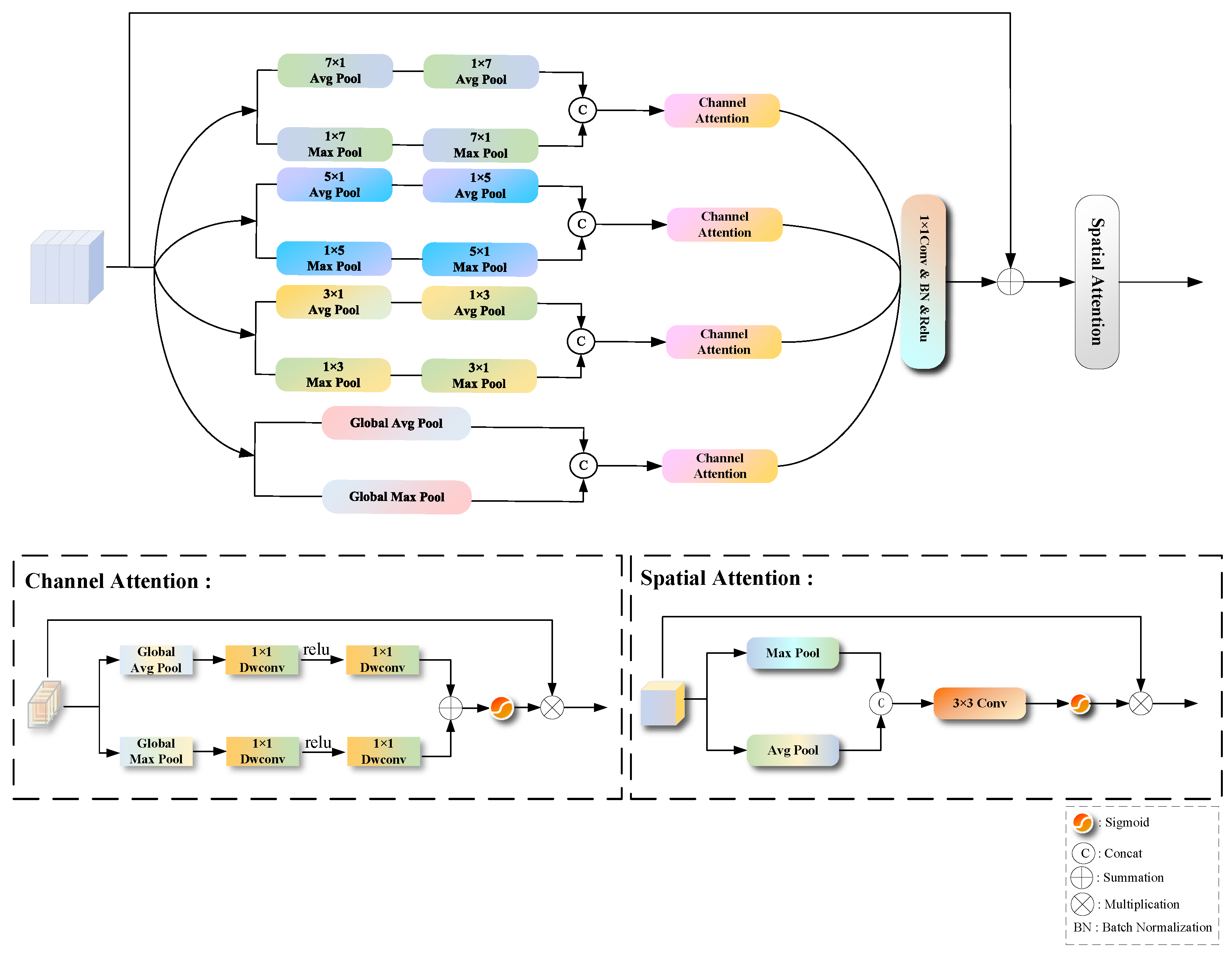
For deep neural networks, capturing long-range dependencies is crucial. However, convolutional operations are limited to processing local regions with a restricted receptive field, making it challenging to capture long-range feature correlations. Using large square-kernel pooling operations can increase the sharing of global information, which is effective at detecting large-scale cloud regions. However, for scattered small-sized cloud clusters, this approach performs poorly. The large square-kernel pooling operation extracts excessive information from irrelevant areas, leading to interference in the model’s final predictions and reducing segmentation accuracy. Additionally, when dealing with the segmentation of closely connected and irregularly shaped junctions between clouds and cloud shadows, typical square-kernel pooling operations cover more pixels, potentially containing more irrelevant information, thereby blurring the edge details of the junctions. In response to the above problems, Hou et al. [17] proposed strip pooling, which can capture long-distance relationships while reducing interference from unrelated areas. Inspired by the above ideas, we propose a deep multi-scale pooling attention module (DMPA), the specific structure of which is shown in Figure 3. After feature extraction by the ResNet18 backbone network, deep features contain higher-level semantic information. The DMPA module further extracts multi-scale contextual semantic information, which is useful for distinguishing different cloud and cloud shadow regions, enabling the model to better differentiate clouds and cloud shadows from the background while identifying fine edges and textures, refining the segmentation of irregular junctions between clouds and cloud shadows. The module simultaneously extracts multi-scale deep spatial information and multi-scale deep channel information, better focusing on the category and positional features of clouds and cloud shadows, thereby enhancing the network’s ability to detect and predict scattered small-sized targets and further improve the segmentation results.
The DMPA module first takes the original feature map and inputs it into a multi-scale strip pooling block. This block consists of four groups of pooling layers: one group of global pooling layers and three groups of strip pooling layers. The global pooling layer includes one branch for global max pooling and one branch for global average pooling. The three groups of strip pooling layers include average pooling branches with pooling kernels of N × 1 and 1 × N (N = 3, 5, 7), and max pooling branches with pooling kernels of 1 × N and N × 1 (N = 3, 5, 7). The strip max pooling emphasizes significant features while ignoring minor information, while the strip average pooling smooths features and retains detailed information. By combining both approaches, their respective strengths are fully utilized, enhancing the segmentation performance.The N × 1 strip pooling tends to learn vertical details in cloud and cloud shadow images, while the 1 × N strip pooling is more inclined to learn horizontal details. This allows for the extraction of both vertical and horizontal edge features in the image. Since the edges of clouds and cloud shadows are often closely connected, these operations can effectively capture the edge feature information at the junctions between clouds and cloud shadows, thus improving the segmentation accuracy at these junctions. Each pooling branch parallelly extracts and adds input features, resulting in multi-scale feature maps. The feature maps are then resized back to the input size and concatenated along the channel dimension, completing the multi-scale strip feature extraction process. Details related to the extraction of the above strip features are shown in Figure 4.
After multi-scale strip pooling block feature extraction, the deep feature map is input into the channel attention mechanism to enhance the model ’s attention and selection of different channel features, so that the model pays more attention to learning useful feature information. The weights obtained by the channel attention branch are processed by 1 × 1 convolution, batch normalization, and Relu nonlinear activation function and then added to the original feature map for residual connection so that the network can learn residual information, so that it is easier to train the deep network, effectively solve the problem of gradient disappearance, and optimize the network. Finally, the weight after feature fusion is input into the spatial attention mechanism to enhance the feature relevance and importance of the model to different spatial positions so that the model pays more attention to the regions related to clouds and cloud shadows in the image, which can effectively help the model to accurately locate the detection target and strengthen the prediction and segmentation of scattered small-sized cloud and cloud shadow.
The core content of the designed channel attention module is to use two types of global pooling to extract advanced features. Global pooling is global average pooling and global maximum pooling, respectively. Using different global pooling means that the extracted advanced features are more abundant. After that, the channel is compressed to 1/8 by a two-dimensional depthwise separable convolution with a convolution kernel of 1. After being weighted by the Relu activation function, the channel is restored by a two-dimensional depthwise separable convolution with a convolution kernel of 1. Since two-dimensional depthwise separable convolution can effectively reduce the number of parameters and improve computational efficiency while maintaining strong feature expression ability and helping the network better focus on details and local information, we use two-dimensional depthwise separable convolution as an extractor of information between channels, focusing on the importance of features in different channels. The above process is expressed by Formulas (2) and (3):
The weights of the two pooling branches are added and re-weighted by the sigmoid function. Finally, the output is multiplied by the initial weight of the input channel attention. Formula (4) can be used to express this.
where denotes the Sigmoid function.
The core content of the designed spatial attention module is to use average pooling and maximum pooling to extract feature information. Unlike the channel attention module, these two aggregation methods in the spatial attention module are carried out along the channel dimension. After connecting the feature map results generated by average pooling and maximum pooling in the channel dimension, a convolution operation with a convolution kernel of 3 × 3 is performed to reduce the number of channels from 2 to 1. Considering that the size of the deepest feature map of the network is the smallest, the convolution with a convolution kernel of 3 × 3 can better preserve the details and capture the local features. Then, the feature map is re-weighted by the nonlinear activation function Sigmoid and multiplied by the weight of the initial input spatial attention to generate the final feature map. The above process is shown in Formula (5):
where denotes the Sigmoid function. represents splicing in the channel dimension, Max pooling is represented by Mp, and average pooling is represented by Ap.
2.4. Boundary Detail Feature Perception Module (BDFP)
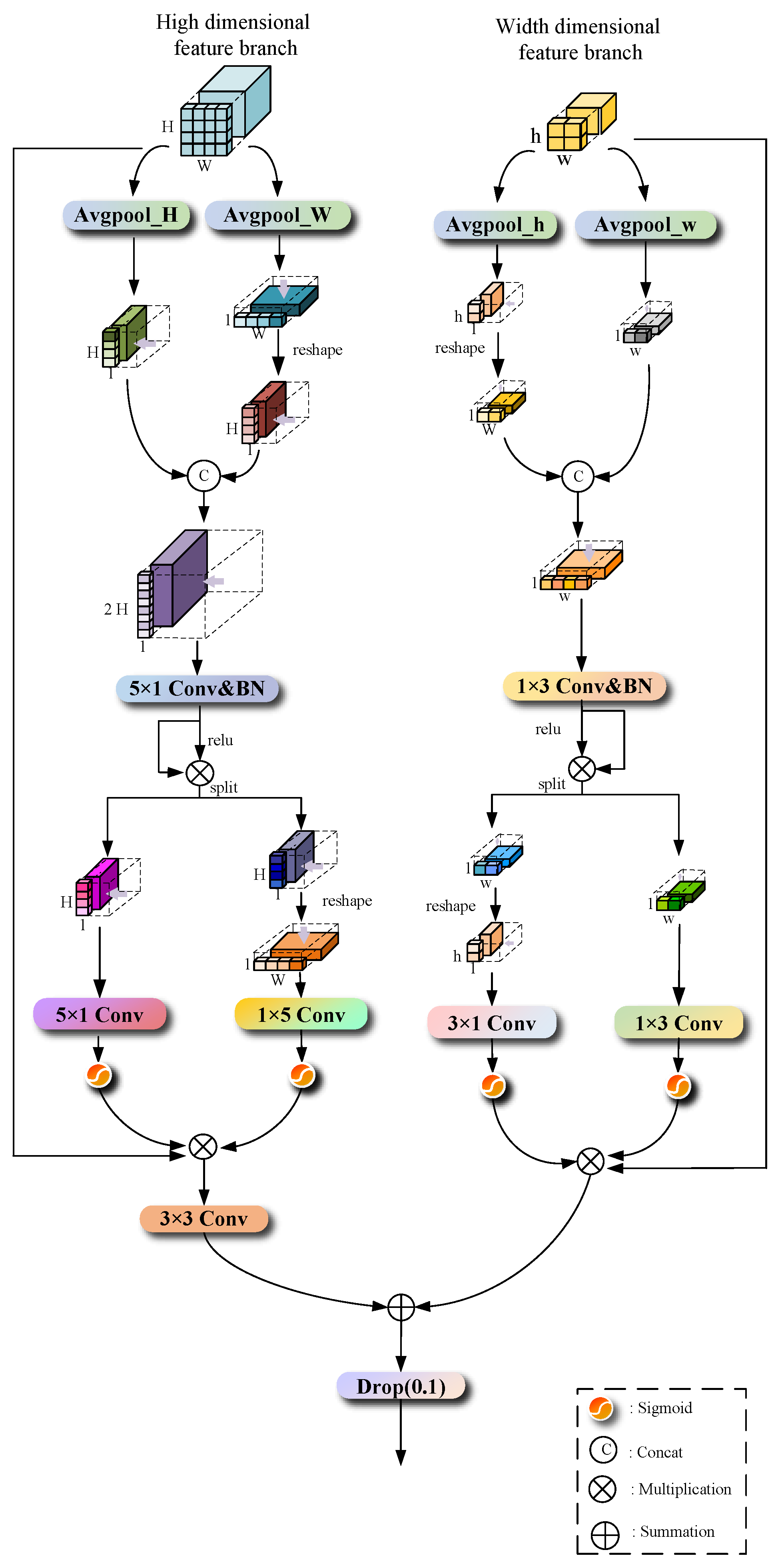
Due to the arbitrary and irregular sizes and shapes of clouds and their shadows, detecting boundary information is challenging, and existing methods [18] often produce coarse segmentation boundaries with insufficient details. To address this issue, we propose the boundary detail feature perception module (BDFP) between the encoder and decoder branches; the specific structure is shown in Figure 5. The BDFP module serves as a skip connection, guiding the fusion of features between adjacent shallow and deep feature maps from the backbone network and then inputting them into the decoder branch. By fusing with high-level decoder features, it helps the decoder to better restore fine details during image pixel restoration. The module consists of two branches: the high dimensional feature branch and the width dimensional feature branch. They, respectively, extract spatial dimension information from the adjacent two layers’ output feature maps of the backbone network, guiding the network to focus on features at different positions in the image. This enhances the model’s ability to model the boundaries, details, and spatial structures of the detected objects, thus refining the boundary segmentation details of clouds and cloud shadows and improving segmentation accuracy.
In the high-dimensional feature branch, the first step is to use two spatial ranges of the pooling kernel (H, 1) or (1, W) to encode along the horizontal and vertical coordinates of the input large-sized feature map x, respectively, preserving the height and width information of the input image. The encoded 1 × W pixel-sized feature map is reshaped into an H × 1 pixel-sized feature map . Then, it is concatenated along the high dimension with another encoded H × 1 pixel-sized feature map to increase the height of the feature map to twice the original height. At this point, it contains richer feature information in the vertical direction. The process is represented by Formula (6):
In Formula (6), represents the concatenation operation along the high dimension. is the feature map obtained after concatenation along the height dimension. Then, a 2D convolution with a kernel size of 5 × 1 is applied, performing convolutional operations along the vertical direction for each position’s pixel to capture features along the height dimension comprehensively. Subsequently, the resulting feature map is processed through batch normalization and then ReLU activation function to reweight the features. It is then element-wise multiplied with the weight obtained from the vertical strip convolution of the high-dimensional features. This process is illustrated by Formulas (7) and (8):
where BN denotes batch normalization. denotes a two-dimensional convolution with a convolution kernel of 5 × 1. represents the nonlinear activation function Relu. Then, we decompose into two independent tensors and ; the two-dimensional convolution with the convolution kernel of 5 × 1 and the two-dimensional convolution with convolution kernel of 1 × 5 are used to extract the height dimension and width dimension features of the decomposed two tensors, respectively. The two tensors are weighted by the Sigmoid function after feature extraction and multiplied by the most original input tensor. We finally obtain that the output of the high-dimensional feature branch can be shown in Formula (9):
where denotes the Sigmoid function. denotes a two-dimensional convolution with a convolution kernel of 1 × 5.
In the width dimension, the feature branch similarly utilizes pooling kernels with two spatial ranges (h, 1) or (1, w) to encode the input small-sized feature map y along the horizontal and vertical coordinate directions separately. This process preserves both the height and width information of the input image. The encoded h × 1 pixel feature map is then transformed through a reshape operation into a 1 × w pixel feature map . This 1 × w pixel feature map is concatenated with another branch’s encoded 1 × w pixel feature map along the width dimension, resulting in the width of the feature map being doubled compared to the input. This process is represented by Formula (10):
where denotes concatenation operation in the width dimension. is the feature map after splicing the width dimension. After that, through the two-dimensional convolution with a convolution kernel of 1 × 3, the pixels at each position are convoluted along the horizontal direction to fully capture the feature information on the width dimension. After that, the same process is first processed by batch normalization and then re-weighted by Relu activation function. The width dimension feature weight after the bar convolution is multiplied by the element by element to perform feature fusion. The process is shown by the Formulas (11) and (12):
where denotes a two-dimensional convolution with a convolution kernel of 1 × 3; then, we decompose into two independent tensors, and , and use the two-dimensional convolution with a convolution kernel of 1 × 3 and the two-dimensional convolution with a convolution kernel of 3 × 1 to extract the width dimension and height dimension features of the decomposed two tensors, respectively. The two tensors are weighted by the Sigmoid function after feature extraction and multiplied by the most original input tensor element by element. We finally obtain that the output of the width dimension feature branch can be shown in Formula (13):
where denotes the Sigmoid function. denotes a two-dimensional convolution with a convolution kernel of 3 × 1.
Because the feature image pixel sizes output by the high-dimensional feature branch and the width-dimensional feature branch are different, the size of the feature map output by the high-dimensional feature branch is twice that of the width-dimensional feature branch. Therefore, before we fuse the features output by the two branches, a two-dimensional convolution with a convolution kernel of 3 × 3 is used to transform the number of channels, and the height and width of the feature map output by the high-dimensional feature branch into the same one as the width-dimensional feature branch. Finally, the feature map after the fusion of the two branches is input into the dropout function. In the prediction stage, the neurons in the probability network of 0.1 can be discarded, which can improve the accuracy of segmentation to a certain extent, obtain a prediction map with good segmentation effect, and prevent network overfitting. The process is shown in Formula (14):
where is the output result feature map, is the dropout function, and is the two-dimensional convolution with a convolution kernel of 3 × 3.
2.5. Cross-Layer Self-Attention Feature Fusion Module (CSFF)
In the task of cloud and cloud shadow segmentation, the thin cloud layer is easy to ignore by the network because its own characteristics are not obvious enough, resulting in missed detection during prediction, and various interferences in the original image will also interfere with the network in predicting the detection target, affecting the segmentation effect. In order to solve this problem, we propose a cross-layer self-attention feature fusion module in the decoding stage, which is used to fuse shallow detail information and deep semantic information, fully extract features, improve the anti-interference ability of the network, improve the attention to thin clouds, reduce the probability of missed detection and false detection, and further realize the accurate prediction and segmentation of cloud and cloud shadow.
A thin cloud is an object that is easily misdetected during the detection process. Therefore, in the detection of thin clouds, the network often needs to provide a larger receptive field [19], and the function of the self-attention mechanism is to extend the receptive field to the entire world. In theory, the self-attention mechanism can establish the spatial location information covering all pixels of the feature map [20]. However, an obvious drawback of the self-attention mechanism is that the amount of computation is large and there is a certain amount of computational redundancy. When we design a cross-layer self-attention feature fusion module, the module is mainly composed of three branches, which are two convolution branches for local feature information extraction through a depthwise separable convolution with a convolution kernel of 3 × 3, and our improved self-attention branch in the middle. We assume that the feature maps from the deep and shallow layers of the network are and , respectively, where the width and height of are twice that of . In the self-attention branch of the CSFF module, we first double upsample the deep small-size feature map , then concatenate the operation with the shallow large-size feature map in the channel dimension, and lastly generate through the layer normalization operation. At the same time, we use the feature information in to generate the query vector (Q), key vector (K), and value vector (V) and use local context information to enrich it. It aggregates pixel-level cross-channel context information by using 1 × 1 convolution. Then, 3 × 3 depthwise separable convolution is used to encode channel-level spatial context information. Our module generates Q, K, and V, as shown in Formulas (15)–(17):
the query vector and key vector are then reshaped to interact with each other so that their dot products can produce a transposed attention graph with size. The procedure described above is as below:
where is the feature map of the self-attention branch output. , , and are obtained from the original size remodeling tensor. Before the Softmax function, the point product size of and is controlled by the learning scaling parameter in this instance. is a Softmax function. R is a symbol for the rearrange operation. For the convolution branch of the CSFF module, the feature map of after upsampling and are input into the depthwise separable convolution with the 3 × 3 convolution, batch normalization, and Relu, respectively, and output as and , respectively. The procedure described above is as follows:
where represents batch normalization and represents double upsampling. Finally, we fuse the feature weights output by the three branches of the CSFF module to further extract the feature information for the decoding stage and promote the image information recovery. The following is its formula:
where Y is the final output feature diagram. Figure 6 shows the CSFF module.
3. Experiment
3.1. Dataset
3.1.1. Cloud and Cloud Shadow Datasets
The cloud and cloud shadow datasets used in this study are obtained from Google Earth, a virtual globe software developed by Google that integrates satellite imagery, aerial photography, and geographic information systems onto a 3D model of the Earth. The global topographic images on Google Earth have an effective resolution of at least 100 m and are typically 30 m in resolution for regions like mainland China, with an observation altitude (Eyealt) of 15 km. The dataset consists of high-resolution remote sensing images randomly collected by professional meteorological experts in various regions, including the Yunnan Plateau, Qinghai Plateau, Tibetan Plateau, and the Yangtze River Delta. To comprehensively evaluate the model’s performance, we selected several sets of high-resolution cloud images captured from different shooting angles and altitudes. The longitude and latitude coordinates of the data collection areas are provided in Table 1.
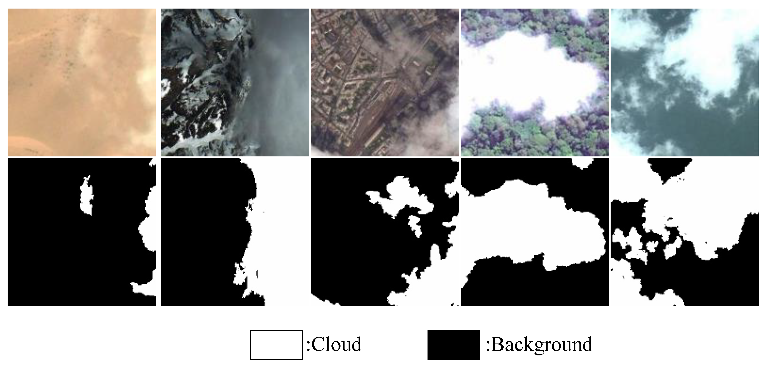
Due to the limitation of GPU video storage capacity, we cut the original high-definition cloud remote sensing image with a resolution of 4800 × 2692 into a size of 224 × 224. After screening (we cleaned the data set and deleted the cloud-free images and cloud-only images), we obtained a total of 12,280 images. We divided the data set into a training set and a validation set according to 8/2. Deep neural networks require a lot of training data, but it is difficult to obtain these learning samples. Therefore, it is necessary to use data augmentation to avoid overfitting when there are few training samples. Therefore, this article used translation, flip, and rotation for data augmentation. After data augmentation, the dataset was expanded to 39,296 training set images and 9824 validation set images, and the ratio of training set and validation set was still 8/2. As shown in Figure 7, the high-resolution cloud and cloud shadow images obtained from Google Earth are roughly divided into five types, which have different backgrounds, namely, waters, forests, fields, towns, and deserts. These tags are manually labeled, and there are three types: cloud (red), cloud shadow (green), and background (black).
3.1.2. HRC_WHU Dataset
In order to further verify the generalization performance of the proposed algorithm, we use the high-resolution cloud dataset HRC_WHU [21] for verification. Images of this dataset were collected from Google Earth. Experts in the field of remote sensing image interpretation of Wuhan University have digitized the relevant reference cloud masks. The dataset contains 150 high-resolution remote sensing images of large scenes. Each image contains three channels of RGB information, distributed in various regions of the world, including deserts, snow, urban, forest, and water. There are five different backgrounds. The image resolution is mainly between 0.5 m and 15 m. The original size of the image is 1280 × 720. Due to the memory limitations of the GPU, we cut the original image into 256 × 256 small-size images for training. After screening, we obtained a total of 5200 images, which were divided into training sets and verification sets according to 8/2. In order to enhance the generalization ability of the model, we performed data augmentation operations through translation, flipping, and rotation. After data augmentation, the data set was expanded to 16,640 training set images and 4160 verification set images. The ratio of the training set and the verification set is still 8/2. Figure 8 shows some images in the HRC_WHU dataset. There are two types of dataset labels: cloud (white) and background (black).
3.1.3. SPARCS Dataset
We use the public dataset SPARCS [22,23] to verify the performance of the proposed method in multi-spectral scenarios. The dataset was originally created by M. Joseph Hughes of Oregon State University and was manually exported from pre-collected Landsat-8 scenes. The dataset contains 80 images of 1000 × 1000 pixels, that is, a subset of pre-collected Landsat-8 scenes, including clouds, cloud shadows, snow/ice, water, and background categories. Due to the limitation of GPU memory, we cut the original data set into small images of 256 × 256 pixels. After screening, we obtained a total of 2000 images, which were divided into a training set and a verification set according to 8/2. In order to enhance the generalization ability of the model, we performed data augmentation operations through translation, flipping, and rotation. After data augmentation, the data set was expanded to 6400 training set images and 1600 verification set images. The ratio of training set and verification set is still 8/2. Figure 9 shows some images in the SPARCS dataset. There are five types of dataset labels: cloud (white), cloud shadow (black), snow/ice (light blue), water (dark blue), and background (gray).
3.2. Experimental Details
Our experimental implementations are based on the public platform PyTorch (Paszke et al., 2017) [24]. In this work, we use the "Steplr" learning rate strategy, that is, . The baseline learning rate is set to 0.001, the adjustment multiple is set to 0.98, and the adjustment interval is set to 3. The number of training times is set to 300, and the cross entropy is used as the maximum loss function. Since the Adam optimizer [25] converges quickly and stably, in the experiments involved in this paper, we use Adam as the optimizer, where is set to 0.9 and is set to 0.999. NVIDIA GeForce RTX 3070 with an 8G storage capacity powers our training system. We set the batch size to 24 for training the cloud and cloud shadow datasets due to the physical memory restriction of a single GPU, and we set the batch size to 18 when training the HRC_WHU dataset and SPARCS dataset. To assess how well our network performs using the cloud shadow dataset, HRC_WHU data, and SPARCS dataset, we selected the following metrics as our assessing indices: mean PA (MPA), pixel accuracy (PA), F1 score, mean intersection over union (MIoU), frequency weighted intersection over union (FWIoU), and the time of training a picture (Time).
3.3. Ablation Experiment
In this section, we first use ResNet18 without opening pre-training as the backbone, and we replace the proposed module with an auxiliary module composed of ordinary convolution and upsampling when the overall network structure remains unchanged and then connect them for output. Next, we gradually add the designed modules’ ( BDFP, CSFF, and DMPA ) replacement auxiliary modules to the network to verify the feasibility of each module and the entire network. Table 2 details the increase in network prediction accuracy for each module.
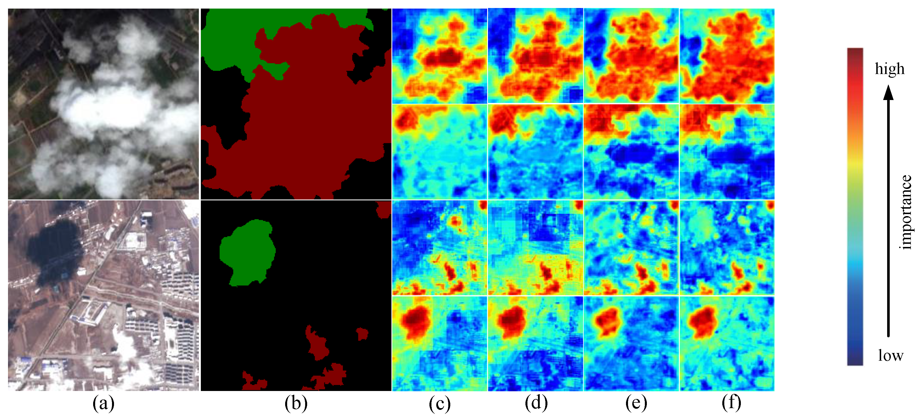
BDFP ablation: The BDFP module separates and combines the spatial dimension data from the feature diagrams produced by the backbone network’s top two layers; this guides our network to focus on the information of different positions in the picture and enhances the modeling ability of the MSFANet to detect the boundary, detail, and spatial structure of the target. According to Table 2, the BDFP module increases MIoU by 0.21%. Through the thermal visualization effect of Figure 10d, we can find that after adding this module, the network focus on the boundary details of the cloud shade, cloud, and the overall prediction effect is significantly improved.
CSFF ablation: The CSFF module utilizes a combination of self-attention mechanism and convolution to effectively integrate a shallow-layer detail feature and deep-layer semantic feature, enabling comprehensive information extraction. According to Table 2, the CSFF module increases the MIoU of the network by 0.65%. Through the thermal visualization effect of the first cloud image under the background of farmland in Figure 10e, it is clear that the addition of the CSFF module helps the network increase its attention to thin clouds. Through the second cloud image of the urban background with interference in Figure 10, we compare the thermal visualization effect before and after adding the CSFF module. Our network now obviously focuses on the predictive information that is most useful, and its anti-interference capability is enhanced as a result of the addition of the CSFF module. As a result, the likelihood of a prediction target being incorrectly detected is decreased. The capacity to identify the image’s interfering objects (such as white house buildings and black building reflections) is also improved.
DMPA ablation: The DMPA module fully extracts the multi-scale strip semantic features and channel spatial features of the deep network and improves MSFANet’s attention to the details of the combination of cloud–cloud shade and the prediction ability of small detection targets. According to Table 2, the DMPA module increases the MIoU of the network by 0.5%. Through the thermal visualization effect of the first cloud image in the farmland background in Figure 10f, we can find that the border connections of cloud–cloud shade can be distinguished significantly more clearly with the help of the DMPA module. The thermal visualization effect of the second cloud image in the urban background with interference in Figure 10f shows that the DMPA module helps MSFANet to catch the scattered small-sized cloud–cloud shade and achieves a more accurate positioning of such small detection targets.
3.4. Comparative Testing of Cloud and Cloud Shadow Datasets
In this section, we compare the proposed method with other semantic segmentation networks, where SP_CSANet [26], PADANet [27], LCDNet [28], and CloudNet [29] are other networks specifically designed for cloud and cloud shadow semantic segmentation tasks. We chose pixel accuracy (PA), mean PA (MPA), F1 score, frequency weighted intersection over union (FWIoU), mean intersection over union (MIoU), and time of training a picture (Time) as evaluating indexes. Table 3 shows the quantitative results of the above indicators. Among all the comparison methods, our network works best. When comparing with other backbone networks without pre-trained semantic segmentation networks, the backbone network of our network does not load pre-trained models, and when comparing with other backbone networks with pre-trained semantic segmentation networks, we load pre-trained models on the backbone network. For the two comparison methods, our network is ahead of other networks in all indicators, which shows the effectiveness of our proposed method. By comparing the time required to train a picture, it can be found that our network takes less time than most other networks, and our network computing performance has certain advantages.
In Figure 11, some illustrations of representative scenarios have been chosen. In the comparison of the effect of the prediction graph, we selected several excellent networks (such as PSPNet, ENet, BiseNetV2, DeepLabV3plus, and Swin_Transformer) with distinct characteristics for comparison to prove the feasibility of our network. In the selected example diagram, we used white frames to mark the different network segmentation results at the same position, so that the segmentation effect of each network is clear at a glance. For example, in the second row of forest background, PSPNet, ENet, BiSeNetV2, DeepLabV3plus, and Swin_Transformer misidentified and failed to detect sporadic, small-scale cloud cover, while our network can accurately predict almost all cloud and cloud shadow in the image. In the third line of desert background, only our network achieves accurate detection of thin clouds in the lower right corner, and other comparison networks have missed detection, indicating that our network focuses on thin clouds and has better performance. In the images displayed in the first line of farmland background and the third line of the fifth line of desert background, in the erratic intersection of cloud–cloud shade, our network significantly outperforms previous comparison networks because of its superior detail segmentation. Through the images displayed in the fourth row of water background and the fifth row of desert background, we can discover that our method is better than other comparison methods in predicting the complex boundary details of cloud–cloud shade. By combining the aforementioned findings, in the presence of diverse environmental background, the BDFP module retrieves and combines the spatial dimension information of the feature maps produced by the backbone’s neighbouer two layers, guiding the network to focus on the position information of different pixels in the picture, and helps the network to enhance the target’s detection’s target’s border detail feature extraction. At the same time, the DMPA module fully extracts the multi-scale strip semantic features and channel spatial features of the deep network and improves MSFANet’s attention to the junction of cloud and cloud shadow and the detection ability of small detection targets. Through the CSFF module, the deeplayer semantic feature and shallow detail feature are combined, the features are fully extracted, the network’s interference prevention is enhanced, and the thin cloud layer is given more consideration. The advantages of our network are further demonstrated by comparison with other traditional networks for picture segmentation in various environmental settings.
Figure 12 displays the prediction effects of several networks when noise is present. We selected five typical images, and we also used white frames in the prediction images to mark different network segmentation results in the same location, which better demonstrated the superiority of our network. As shown in the first row, the results show that when there is an interfering object in the original image, except when our network does not have that interfering object (black land) mistakenly detected as a cloud shadow, other comparison networks have produced false detection, reflecting the fact that our CSFF module promotes the full interaction of information at different layers, thereby improving the network’s resistance to interfering objects and achieving the accurate judgment and prediction of detection targets. As seen in the 2nd line and the 3rd row of the segmentation results, we intuitively find that the PSPNet, ENet, BiseNetV2, DeepLabV3plus, and Swin_Transformer deal with the cloud border features, and the irregular cloud–cloud shade junction is visible when there is a lot of interference caused by noise, the effect of which is unsatisfactory. However, our network is very effective in detail processing in this respect. The prediction effect diagram shown in the 3rd, 4th, and 5th lines indicates that when the original picture has much noise interference, except when our network achieves the accurate prediction of scattered distribution of small size clouds and cloud shade, other networks of comparison have more or less missed detection, which proves the good prediction performance of our network for such difficult-to-detect targets. The above comparison results show that despite the fact that the cloud layer of the image has a lot of noise interference and there are also interferences that share similarities in pigmentation and shape on the ground, with the help of the DMPA module, our network can acquire a deep multi-scale feature, channel space information, the accurate prediction of scattered small-scale detection targets, and the detailed segmentation of the complex combination of cloud and cloud shadow. With the BDFP module, the network extracts and fuses the spatial dimension information to acquire the boundary detail features of the detection target and can create a more precise categorisation when segmenting the edge details of cloud and cloud shadow. Based on the above analysis, when there are noise and other interferences in the original image, our network can still maintain good performance.
3.5. Generalization Experiment of HRC_WHU Dataset
In order to further prove the effectiveness of our proposed method, we also conducted generalization experiments on the HRC_WHU dataset. We chose pixel accuracy (PA), mean PA (MPA), F1 score, frequency weighted intersection over union (FWIoU), and mean intersection over union (MIoU) as evaluating indexes. The experimental results are shown in Table 4. Among all the comparison methods, the prediction of cloud segmentation in our network works best. When compared with other backbone networks without pre-trained semantic segmentation networks, the backbone network of our network does not load pre-trained models, and when compared with other backbone networks with pre-trained semantic segmentation networks, we load pre-trained models on the backbone network. Regarding the HRC_WHU dataset, our network is ahead of other networks in all indicators, which shows the effectiveness of our proposed method.
Figure 13 depicts the prediction effect of different methods on clouds under various conditions. The background of the image is deserts, snow, urban, forest, and water from top to bottom. Through the first line of the display map, we can find that when predicting and segmenting the shape of large thick clouds, the BDFP module extracts and fuses the spatial dimension information of the feature diagram, guides MSFANet to catch the features of different positions in the image, and helps our network. The boundary details of the cloud are fully preserved, and the segmentation is detailed. Other networks have the issue of blurred boundary detail prediction and rough segmentation. The second line of the display map is to select the segmentation of the thin cloud layer under the snow background. The snow has similar color and shape features to the cloud, which can easily cause interference when the network predicts the cloud. In view of the interference problem, our CSFF module promotes the full interaction of information in different layers, thereby improving the network’s capability to prevent interference, and can achieve accurate judgment and prediction of detection targets. While avoiding false detection, the prediction of thin cloud shape is also the best. PSPNet introduces PPM, captures context information at different scales, and enhances the perception of clouds; to a certain extent, it improves its anti-interference ability, but the segmentation of cloud boundary details is still worse than our network. The bilateral guided aggregation layer used by BiSeNetV2 also promotes information fusion and improves its anti-interference ability to a certain extent; however, due to insufficient semantic feature extraction, the shape of the cloud cannot be fully restored. The third line predicts the cloud shape and boundary details. It is evident that our network has the advantages of cloud shape and boundary detail segmentation. Regarding the fourth and fifth lines’ results of the forecast, in addition to the comparison, we find that our network has the best effect on the cloud’s shape; it is also clear that MSFANet accurately predicts the scattered small-sized clouds, which is attributed to the DMPA module. Fully extracting deep multi-scale context information helps the network to distinguish the subtle edges and textures of the cloud from the background, and extracting channel spatial information better focuses on the category features and location features of the cloud, which enhances the network’s capture and prediction of scattered small-sized detection targets. All of the other networks have the problems of the missing detection of clouds and the rough shape prediction of clouds. The results of the comparisons mentioned above demonstrate that our network performs very well in cloud prediction and segmentation, and its accuracy effect is superior to that of other comparison networks.
3.6. Generalization Experiment of SPARCS Dataset
In order to further prove the segmentation performance of our method for multispectral remote sensing images, generalization experiments are performed using the SPARCS dataset. We chose pixel accuracy (PA), mean PA (MPA), F1 score, frequency weighted intersection over union (FWIoU), and mean intersection over union (MIoU) as evaluating indexes. Table 5 shows the evaluation results of different networks of the data set. It can be seen from the table that after adding other categories, our method can still maintain the highest accuracy, and the detection ability of cloud and cloud shadow is far more than other methods.
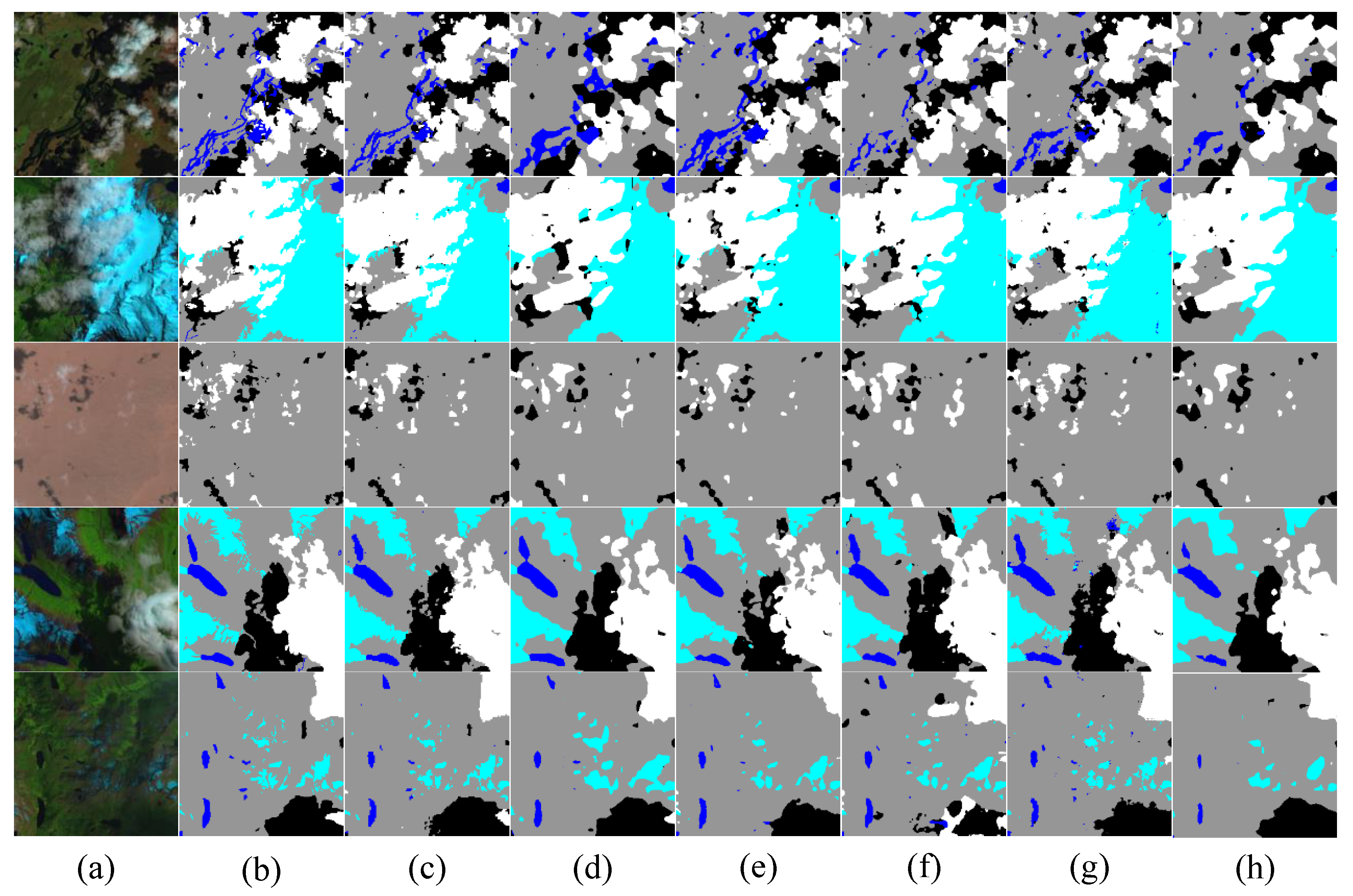
Figure 14 displays the SPARCS dataset’s segmentation results using several approaches. The images displayed contain rich categories, including scattered small clouds, cloud shadow, ice and snow, rivers, and large clouds. Since the background is complicated and contains many categories, identifying small targets and predicting the complex boundary details of detected targets are great challenges. For example, in the renderings shown in the first, second, and fourth rows, we can find that when segmenting the boundary of clouds, rivers, cloud shade, and snow, compared with other networks such as PSPNet and Swin_Transformer, our network can predict the shape boundary details of the detected target to the greatest extent and has the best performance. The third line and the fifth line show the effect diagram. Through comparison, we find that our network has the best effect when predicting scattered small detection targets, which can achieve accurate positioning and retain the shape boundary details of small size detection targets to a large extent. With the extraction of muilti-scale context information, PSPNet enhances its ability to capture small scattered detection targets. In other comparison networks, PSPNet has the least missed detection errors when predicting small detection targets, but it predicts the shape and boundary details of the detection targets. Roughly speaking, the accuracy is lower than our network. Other comparison networks largely have more missed detection and false detection when predicting small detection targets with scattered distribution, and the shape prediction of small detection targets is very rough. The aforementioned comparison findings demonstrate that our network also has benefits and provides the best results for jobs involving multi-classification multi-spectral remote sensing picture segmentation.
4. Discussion
In this part, we compare PSPNet, ENet, BiSeNetV2, DeepLabV3plus, and Swin_Transformer with our network. PSPNet can better understand the global and local relationships in the image by using the pyramid pooling module to capture context information at different scales. This is very important for cloud and cloud shadow semantic segmentation because the shape and size of the cloud can vary greatly in the image, but PSPNet is rough in the segmentation of the target boundary, which needs post-processing to solve, especially in the case of fuzzy boundaries. Our DMPA module further extracts multi-scale contextual semantic information to help the model better distinguish clouds and cloud shadows, distinguish subtle edges and textures from the background, and refine the segmentation of the irregular junction of clouds and cloud shadows. And our network requires less computing time than PSPNet, which has better performance than PSPNet. The design of ENet aims to keep the model lightweight and reduce the computational and memory requirements. However, some performance is sacrificed on the segmentation accuracy details. Missing detection and false detection may occur when predicting small detection targets, and the segmentation boundary details are not clear enough. Our network almost achieves zero error detection and zero leakage detection when detecting scattered small detection targets, and the BDFP module improves the modeling ability of the network to detect the boundary, detail, and spatial structure of the target and helps the network to refine the boundary segmentation details of the cloud and cloud shadow and improve the segmentation accuracy. BiSeNetV2 uses the bilateral guided aggregation layer to extract and fuse details and semantic information, which can effectively capture the context information of different scales and help to better understand the scene of cloud and cloud shadow. However, BiSeNetV2 still has high computational complexity to a certain extent, which requires more computing resources and time to train and reason. Our network designs a cross-layer self-attention feature fusion module (CSFF) to fuse shallow detail information and deep semantic information, fully extract features, improve the anti-interference ability of the network, improve the attention to thin clouds, reduce the probability of missed detection and false detection, and further realize accurate prediction and segmentation of clouds and cloud shadows. And our network has advantages in computing time. DeepLabV3plus uses an ASPP module composed of atrous convolutions with different atrous rates to capture context information of different receptive fields. This helps the model to better understand the scene of clouds and cloud shadows, especially for large-scale cloud semantic segmentation tasks, but DeepLabV3plus is usually a relatively large model that requires more computing resources and memory. This may pose challenges in a resource-constrained environment. Our network also has an advantage over DeepLabV3plus in computing time. Swin_Transformer proposes shifted windows; the shifted windowing scheme brings greater efficiency by limiting self-attention computation to non-overlapping local windows while also allowing for cross-window connection. However, through our experiments, it is proved that Swin_Transformer has a poor detection effect on the detection target when there is interference in the original image, and there are problems such as false detection and rough edge detection. Our network uses the cross-layer self-attention feature fusion module (CSFF) to guide the fusion of deep semantic information and shallow detail information. The graph of deep features can provide semantic information for the graph of shallow features. The graph of shallow features will make up for the lack of detail information in the graph of deep features, which improves the anti-interference ability of the network, and our network is superior to Swin_Transformer in calculation time. In summary, compared with these existing networks, my proposed MSFANet has better prediction accuracy and computational efficiency and is in a leading position compared with other similar studies.
Artificial intelligence is playing an increasingly important role in remote sensing. The application of artificial intelligence, especially machine learning algorithms, from initial image processing to high-level data is facilitating understanding and knowledge discovery. Artificial intelligence technology has become a powerful strategy for analyzing remote sensing data and has made significant breakthroughs in all remote sensing fields [36]. The application of artificial intelligence technology in the design of image processing system will promote the automation of image analysis process. Remote sensing applications such as intelligent spaceborne processing, advanced database queries, and the automatic analysis of multispectral images demonstrate the potential of the successful implementation of artificial intelligence technology [37].
5. Conclusions
In this paper, we propose a multi-scale strip feature attention network to achieve end-to-end cloud and cloud shadow detection in high-resolution images of visible spectrum. This method uses ResNet18 as the backbone to mine different levels of semantic information. Then, the deep-layer multi-scale pooling attention module (DMPA) is used to further extract the multi-scale context semantic information, deep channel feature information, and deep spatial feature information. Strip maximum pooling can emphasize salient features and ignore secondary information, strip average pooling can smooth features and retain detailed information, and the combination of the two can give full play to their advantages and improve their segmentation effect. At the same time, a boundary detail feature perception module (BDFP) is proposed between the encoder branch and the decoder branch to play the role of skipconnection. The features of the shallow and deep feature maps adjacent to the backbone network are guided and fused with each other and input into the decoder branch, which is fused with the high-level features of the decoder. The BDFP module extracts the spatial dimension information of the feature map output from the adjacent two layers of the backbone network; guides the network to focus on the features of different positions in the image; improves the modeling ability of the model to detect the boundary, details, and spatial structure of the target; and helps the network refine the boundary segmentation details of clouds and cloud shadows to improve the segmentation accuracy. Finally, in the decoding stage, a cross-layer self-attention feature fusion module (CSFF) is proposed, which fuses shallow detail information and deep semantic information for feature extraction while performing pixel restoration on the image. The CSFF module mainly uses the self-attention mechanism to establish spatial location information that covers all of the pixels of the feature map, providing a larger receptive field for our network. The experimental results show that compared with other networks, our network significantly improves the accuracy of the network, can cope with various complex scenes, and has strong resistance to interference in the image. Our network obtains 93.70% MIoU on the cloud and cloud shadow datasets when backbone does not turn on pre-training, 90.85% MIoU on the HRC_WHU dataset, and 81.66% MIoU on the SPARCS dataset. When backbone turns on pre-training, it obtains 94.65% MIoU on the cloud and cloud shadow datasets, 91.55% MIoU on the HRC_WHU dataset, and 82.18% MIoU the on SPARCS dataset. The data show that our network has good practical application prospects. Although our method has the highest detection accuracy, there is still much room regarding the optimization of our model parameters. Our future research work will focus on reducing the parameters of the model while ensuring the accuracy of the model and minimizing the weight of the model.
Author Contributions
Conceptualisation, K.C., M.X. and K.H.; methodology, M.X. and L.W.; software, X.D., K.C. and K.H.; validation, L.W. and H.L.; formal analysis, M.X., K.C. and K.H.; investigation, K.C. and K.H.; resources, M.X. and L.W.; data curation, K.C. and K.H.; writing—original draft preparation, K.C. and K.H.; writing—review and editing, M.X.; visualisation, X.D.; supervision, M.X.; project administration, M.X.; and funding acquisition, M.X. All authors have read and agreed to the published version of the manuscript.
Funding
This research was funded by the National Natural Science Foundation of PR China of grant number 42075130.
Institutional Review Board Statement
Not applicable.
Informed Consent Statement
Not applicable.
Data Availability Statement
The data and the code of this study are available from the corresponding author upon request.
Conflicts of Interest
The authors declare no conflict of interest.
References
- Zhang, Y.; Rossow, W.B.; Lacis, A.A.; Oinas, V.; Mishchenko, M.I. Calculation of radiative fluxes from the surface to top of atmosphere based on ISCCP and other global data sets: Refinements of the radiative transfer model and the input data. J. Geophys. Res. Atmos. 2004, 109, D19. [Google Scholar] [CrossRef]
- Goodman, A.; Henderson-Sellers, A. Cloud detection and analysis: A review of recent progress. Atmos. Res. 1988, 21, 203–228. [Google Scholar] [CrossRef]
- Pankiewicz, G. Pattern recognition techniques for the identification of cloud and cloud systems. Meteorol. Appl. 1995, 2, 257–271. [Google Scholar] [CrossRef]
- Oishi, Y.; Ishida, H.; Nakamura, R. A new Landsat 8 cloud discrimination algorithm using thresholding tests. Int. J. Remote Sens. 2018, 39, 9113–9133. [Google Scholar] [CrossRef]
- Luo, Y.; Trishchenko, A.P.; Khlopenkov, K.V. Developing clear-sky, cloud and cloud shadow mask for producing clear-sky composites at 250-meter spatial resolution for the seven MODIS land bands over Canada and North America. Remote Sens. Environ. 2008, 112, 4167–4185. [Google Scholar] [CrossRef]
- Main-Knorn, M.; Pflug, B.; Louis, J.; Debaecker, V.; Müller-Wilm, U.; Gascon, F. Sen2Cor for sentinel-2. In Proceedings of the Image and Signal Processing for Remote Sensing XXIII. International Society for Optics and Photonics, Warsaw, Poland, 11–13 September 2017; Volume 10427, p. 1042704. [Google Scholar]
- Hutchison, K.D.; Mahoney, R.L.; Vermote, E.F.; Kopp, T.J.; Jackson, J.M.; Sei, A.; Iisager, B.D. A geometry-based approach to identifying cloud shadows in the VIIRS cloud mask algorithm for NPOESS. J. Atmos. Ocean. Technol. 2009, 26, 1388–1397. [Google Scholar] [CrossRef]
- Zhu, Z.; Woodcock, C.E. Object-based cloud and cloud shadow detection in Landsat imagery. Remote Sens. Environ. 2012, 118, 83–94. [Google Scholar] [CrossRef]
- Cheng, G.; Wang, Y.; Xu, S.; Wang, H.; Xiang, S.; Pan, C. Automatic road detection and centerline extraction via cascaded end-to-end convolutional neural network. IEEE Trans. Geosci. Remote Sens. 2017, 55, 3322–3337. [Google Scholar] [CrossRef]
- Ji, H.; Xia, M.; Zhang, D.; Lin, H. Multi-Supervised Feature Fusion Attention Network for Clouds and Shadows Detection. ISPRS Int. J. Geo-Inf. 2023, 12, 247. [Google Scholar] [CrossRef]
- Long, J.; Shelhamer, E.; Darrell, T. fully convolutional networks for semantic segmentation. In Proceedings of the IEEE Conference on Computer Vision and Pattern Recognition, Boston, MA, USA, 7–12 June 2015; pp. 3431–3440. [Google Scholar]
- Ronneberger, O.; Fischer, P.; Brox, T. U-net: Convolutional networks for biomedical image segmentation. In Proceedings of the International Conference on Medical image Computing and Computer-Assisted Intervention, Munich, Germany, 5–9 October 2015; Springer: Berlin/Heidelberg, Germany, 2015; pp. 234–241. [Google Scholar]
- Zhao, H.; Shi, J.; Qi, X.; Wang, X.; Jia, J. Pyramid scene parsing network. In Proceedings of the IEEE Conference on Computer Vision and Pattern Recognition, Honolulu, HI, USA, 21–26 July 2017; pp. 2881–2890. [Google Scholar]
- Chen, L.C.; Zhu, Y.; Papandreou, G.; Schroff, F.; Adam, H. Encoder-decoder with atrous separable convolution for semantic image segmentation. In Proceedings of the European conference on Computer Vision (ECCV), Munich, Germany, 8–14 September 2018; pp. 801–818. [Google Scholar]
- Zhang, X.; Yu, W.; Pun, M.O. Multilevel deformable attention-aggregated networks for change detection in bitemporal remote sensing imagery. IEEE Trans. Geosci. Remote Sens. 2022, 60, 1–18. [Google Scholar] [CrossRef]
- He, K.; Zhang, X.; Ren, S.; Sun, J. Deep residual learning for image recognition. In Proceedings of the IEEE Conference on Computer Vision and Pattern Recognition, Las Vegas, NV, USA, 27–30 June 2016; pp. 770–778. [Google Scholar]
- Hou, Q.; Zhang, L.; Cheng, M.M.; Feng, J. Strip pooling: Rethinking spatial pooling for scene parsing. In Proceedings of the IEEE/CVF Conference on Computer Vision and Pattern Recognition, Seattle, WA, USA, 13–19 June 2020; pp. 4003–4012. [Google Scholar]
- Li, H.; Xiong, P.; An, J.; Wang, L. Pyramid attention network for semantic segmentation. arXiv 2018, arXiv:1805.10180. [Google Scholar]
- Zhang, Y.; Guindon, B.; Cihlar, J. An image transform to characterize and compensate for spatial variations in thin cloud contamination of Landsat images. Remote Sens. Environ. 2002, 82, 173–187. [Google Scholar] [CrossRef]
- Wang, X.; Girshick, R.; Gupta, A.; He, K. Non-local neural networks. In Proceedings of the IEEE Conference on Computer Vision and Pattern Recognition, Salt Lake City, UT, USA, 18–22 June 2018; pp. 7794–7803. [Google Scholar]
- Li, Z.; Shen, H.; Cheng, Q.; Liu, Y.; You, S.; He, Z. Deep learning based cloud detection for remote sensing images by the fusion of multi-scale convolutional features. arXiv 2018, arXiv:1810.05801. [Google Scholar]
- Hughes, M.J.; Hayes, D.J. Automated detection of cloud and cloud shadow in single-date Landsat imagery using neural networks and spatial post-processing. Remote Sens. 2014, 6, 4907–4926. [Google Scholar] [CrossRef]
- Hughes, M. L8 SPARCS Cloud Validation Masks; US Geological Survey: Sioux Falls, SD, USA, 2016.
- Paszke, A.; Gross, S.; Chintala, S.; Chanan, G.; Yang, E.; DeVito, Z.; Lin, Z.; Desmaison, A.; Antiga, L.; Lerer, A. Automatic Differentiation in Pytorch. 2017. Available online: https://openreview.net/forum?id=BJJsrmfCZ (accessed on 14 August 2023).
- Kingma, D.P.; Ba, J. Adam: A method for stochastic optimization. arXiv 2014, arXiv:1412.6980. [Google Scholar]
- Qu, Y.; Xia, M.; Zhang, Y. Strip pooling channel spatial attention network for the segmentation of cloud and cloud shadow. Comput. Geosci. 2021, 157, 104940. [Google Scholar] [CrossRef]
- Xia, M.; Qu, Y.; Lin, H. PANDA: Parallel asymmetric network with double attention for cloud and its shadow detection. J. Appl. Remote Sens. 2021, 15, 046512. [Google Scholar] [CrossRef]
- Hu, K.; Zhang, D.; Xia, M.; Qian, M.; Chen, B. LCDNet: Light-Weighted Cloud Detection Network for High-Resolution Remote Sensing Images. IEEE J. Sel. Top. Appl. Earth Obs. Remote Sens. 2022, 15, 4809–4823. [Google Scholar] [CrossRef]
- Xia, M.; Wang, T.; Zhang, Y.; Liu, J.; Xu, Y. Cloud/shadow segmentation based on global attention feature fusion residual network for remote sensing imagery. Int. J. Remote Sens. 2021, 42, 2022–2045. [Google Scholar] [CrossRef]
- Liu, Z.; Lin, Y.; Cao, Y.; Hu, H.; Wei, Y.; Zhang, Z.; Lin, S.; Guo, B. Swin transformer: Hierarchical vision transformer using shifted windows. In Proceedings of the IEEE/CVF International Conference on Computer Vision, Montreal, BC, Canada, 11–17 October 2021; pp. 10012–10022. [Google Scholar]
- Yang, M.; Yu, K.; Zhang, C.; Li, Z.; Yang, K. Denseaspp for semantic segmentation in street scenes. In Proceedings of the IEEE Conference on Computer Vision and Pattern Recognition, Salt Lake City, UT, USA, 18–22 June 2018; pp. 3684–3692. [Google Scholar]
- Pang, K.; Weng, L.; Zhang, Y.; Liu, J.; Lin, H.; Xia, M. SGBNet: An ultra light-weight network for real-time semantic segmentation of land cover. Int. J. Remote Sens. 2022, 43, 5917–5939. [Google Scholar] [CrossRef]
- Yu, C.; Gao, C.; Wang, J.; Yu, G.; Shen, C.; Sang, N. Bisenet v2: Bilateral network with guided aggregation for real-time semantic segmentation. Int. J. Comput. Vis. 2021, 129, 3051–3068. [Google Scholar] [CrossRef]
- Wang, W.; Xie, E.; Li, X.; Fan, D.P.; Song, K.; Liang, D.; Lu, T.; Luo, P.; Shao, L. Pyramid vision transformer: A versatile backbone for dense prediction without convolutions. In Proceedings of the IEEE/CVF International Conference on Computer Vision, Montreal, BC, Canada, 11–17 October 2021; pp. 568–578. [Google Scholar]
- Paszke, A.; Chaurasia, A.; Kim, S.; Culurciello, E. Enet: A deep neural network architecture for real-time semantic segmentation. arXiv 2016, arXiv:1606.02147. [Google Scholar]
- Zhang, L.; Zhang, L. Artificial intelligence for remote sensing data analysis: A review of challenges and opportunities. IEEE Geosci. Remote Sens. Mag. 2022, 10, 270–294. [Google Scholar] [CrossRef]
- Estes, J.E.; Sailer, C.; Tinney, L.R. Applications of artificial intelligence techniques to remote sensing. Prof. Geogr. 1986, 38, 133–141. [Google Scholar] [CrossRef]
Figure 1.
MSFANet structure diagram.

Figure 2.
Resnet18 residual structure.

Figure 3.
Deep-layer multi-scale pooling attention module structure diagram.

Figure 4.
Strip feature diagram. Where N = 3, 5, and 7.

Figure 5.
Boundary detail feature perception module structure diagram.

Figure 6.
Cross-layer self-attention feature fusion module structure diagram.

Figure 7.
Part of cloud and cloud shadow datasets display.

Figure 8.
Part of HRC_WHU dataset display.

Figure 9.
Part of SPARCS dataset display.

Figure 10.
Display of heat map. (a) Image; (b) label; (c) Resnet18; (d) Resnet18+BDFP; (e) Resnet18 + BDFP + CSFF; and (f) Resnet18 + BDFP + CSFF + DMPA. The 1st row is the attention to the cloud, and the 2nd row is the attention to the cloud shade.
Figure 10.
Display of heat map. (a) Image; (b) label; (c) Resnet18; (d) Resnet18+BDFP; (e) Resnet18 + BDFP + CSFF; and (f) Resnet18 + BDFP + CSFF + DMPA. The 1st row is the attention to the cloud, and the 2nd row is the attention to the cloud shade.

Figure 11.
Comparing the segmentation outcomes of several networks in various environmental contexts using the cloud–cloud shade dataset. (a) Images; (b) labels; (c) MSFANet; (d) PSPNet; (e) ENet; (f) BiseNetV2; (g) DeepLabV3plus; and (h) Swin_Transformer.
Figure 11.
Comparing the segmentation outcomes of several networks in various environmental contexts using the cloud–cloud shade dataset. (a) Images; (b) labels; (c) MSFANet; (d) PSPNet; (e) ENet; (f) BiseNetV2; (g) DeepLabV3plus; and (h) Swin_Transformer.

Figure 12.
Comparison of multiple network segmentation effects on the cloud and cloud shadow datasets under noise. (a) Images; (b) Labels; (c) MSFANet; (d) PSPNet; (e) ENet; (f) BiseNetV2; (g) DeepLabV3plus; and (h) Swin_Transformer.
Figure 12.
Comparison of multiple network segmentation effects on the cloud and cloud shadow datasets under noise. (a) Images; (b) Labels; (c) MSFANet; (d) PSPNet; (e) ENet; (f) BiseNetV2; (g) DeepLabV3plus; and (h) Swin_Transformer.

Figure 13.
Effects of various networks’ segmentation on the HRC_WHU dataset in comparison with various environments. (a) Images; (b) labels; (c) MSFANet; (d) PSPNet; (e) ENet; (f) BiseNetV2; (g) DeepLabV3plus; and (h) Swin_Transformer.
Figure 13.
Effects of various networks’ segmentation on the HRC_WHU dataset in comparison with various environments. (a) Images; (b) labels; (c) MSFANet; (d) PSPNet; (e) ENet; (f) BiseNetV2; (g) DeepLabV3plus; and (h) Swin_Transformer.

Figure 14.
Segmentation impacts of various networks on the SPARCS dataset are compared. (a) Test images; (b) labels; (c) MSFANet; (d) PSPNet; (e) Swin_Transformer; (f) DeepLabV3plus; and (g) ENet; (h) BiseNetV2.
Figure 14.
Segmentation impacts of various networks on the SPARCS dataset are compared. (a) Test images; (b) labels; (c) MSFANet; (d) PSPNet; (e) Swin_Transformer; (f) DeepLabV3plus; and (g) ENet; (h) BiseNetV2.


Table 1.
The location’s latitude and longitude are collected in the data set.
| Background | South to North | West to East |
|---|---|---|
| Water | 30°53′4.48″N to 31°35′46.19″N | 119°47′34.52″E to 120°49′43.81″E |
| Water, City | 31°20′1.32″N to 31°46′25.27″N | 117°27′46.75″E to 117°58′1.24″E |
| City | 32°19′56.28″N to 33°26′13.11″N | 120°28′46.49″E to 121°38′22.05″E |
| Vegetation | 26°47′38.87″N to 27°58′2.12″N | 107°19′35.11″E to 109°32′55.19″E |
| Wasteland | 29°52′53.25″N to 30°45′46.22″N | 88°10′12.45″E to 89°18′10.76″E |
| Wasteland | 41°2′27.26″N to 41°52′47.26″N | 91°54′25.23″E to 92°3′53.14″E |
Table 2.
Gradual use of the designed modules to compare the performance of the network.
| Methods | MIoU (%) |
|---|---|
| ResNet18 | 92.34 |
| Resnet18 + BDFP | 92.55 |
| Resnet18 + BDFP + CSFF | 93.20 |
| Resnet18 + BDFP + CSFF + DMPA | 93.70 |
Table 3.
The comparison results of different network evaluation indexes of cloud and cloud shadow datasets. “+” is used to indicate the pre-trained network (bold indicates the highest outcome)).
Table 3.
The comparison results of different network evaluation indexes of cloud and cloud shadow datasets. “+” is used to indicate the pre-trained network (bold indicates the highest outcome)).
| Methods | PA(%) | MPA(%) | F1(%) | FWIoU(%) | MIoU(%) | Time(ms) |
|---|---|---|---|---|---|---|
| Swin_Transformer [30] | 96.10 | 95.33 | 92.97 | 92.53 | 90.93 | 16.98 |
| UNet [12] | 96.13 | 95.53 | 92.92 | 92.57 | 90.96 | 3.26 |
| DenseAspp [31] | 96.22 | 95.13 | 93.37 | 92.76 | 91.21 | 15.03 |
| DeepLabv3plus [14] | 96.32 | 95.65 | 93.33 | 92.92 | 91.41 | 9.50 |
| SGBNet [32] | 96.39 | 95.44 | 93.53 | 93.06 | 91.51 | 7.93 |
| PADANet [27] | 96.44 | 95.55 | 93.63 | 93.16 | 91.66 | 9.45 |
| FCN8s [11] | 96.46 | 95.51 | 93.71 | 93.21 | 91.71 | 2.97 |
| SP_CSANet [26] | 96.48 | 95.61 | 93.70 | 93.24 | 91.76 | 16.45 |
| BiseNetv2 [33] | 96.55 | 96.07 | 93.66 | 93.34 | 91.92 | 7.29 |
| PVT [34] | 96.60 | 95.64 | 93.49 | 93.46 | 92.00 | 12.83 |
| LCDNet [28] | 96.67 | 96.04 | 93.96 | 93.58 | 92.19 | 6.35 |
| CloudNet [29] | 96.69 | 96.11 | 93.99 | 93.61 | 92.24 | 5.21 |
| ENet [35] | 96.74 | 95.84 | 94.05 | 93.72 | 92.33 | 1.69 |
| PSPNet [13] | 96.80 | 96.45 | 94.06 | 93.80 | 92.47 | 7.96 |
| MSFANet | 97.34 | 96.84 | 95.15 | 94.83 | 93.70 | 2.55 |
| 97.04 | 96.46 | 94.67 | 94.28 | 93.07 | 2.97 | |
| 97.12 | 96.55 | 94.79 | 94.42 | 93.22 | 7.96 | |
| 97.74 | 97.34 | 95.88 | 95.59 | 94.65 | 2.55 |
Table 4.
The comparison results of different network evaluation indexes of HRC_WHU data set. “+” is used to indicate the pre-trained network. (Bold indicates the highest outcome))).
Table 4.
The comparison results of different network evaluation indexes of HRC_WHU data set. “+” is used to indicate the pre-trained network. (Bold indicates the highest outcome))).
| Methods | PA(%) | MPA(%) | F1(%) | FWIoU(%) | MIoU(%) |
|---|---|---|---|---|---|
| FCN8s | 93.30 | 93.03 | 89.98 | 87.48 | 87.06 |
| Swin_Transformer | 93.64 | 93.06 | 90.55 | 88.11 | 87.59 |
| UNet | 93.95 | 93.85 | 90.89 | 88.60 | 88.27 |
| PVT | 94.23 | 93.96 | 91.32 | 89.11 | 88.73 |
| DeepLabv3plus | 94.33 | 94.05 | 91.48 | 89.23 | 88.92 |
| SGBNet | 94.32 | 94.30 | 91.41 | 89.25 | 88.96 |
| LCDNet | 94.51 | 94.36 | 91.71 | 89.59 | 89.27 |
| DenseAspp | 94.53 | 94.44 | 91.74 | 89.64 | 89.33 |
| CloudNet | 94.61 | 94.40 | 91.88 | 89.79 | 89.45 |
| BiseNetv2 | 94.64 | 94.60 | 91.88 | 89.82 | 89.53 |
| ENet | 94.66 | 94.63 | 91.91 | 89.86 | 89.57 |
| SP_CSANet | 94.72 | 94.53 | 92.03 | 89.98 | 89.65 |
| PADANet | 94.73 | 94.56 | 92.05 | 90.01 | 89.69 |
| PSPNet | 94.74 | 94.66 | 92.02 | 89.99 | 89.70 |
| MSFANet | 95.35 | 95.25 | 92.95 | 91.12 | 90.85 |
| ine | 93.93 | 93.90 | 90.85 | 88.56 | 88.24 |
| 95.09 | 94.83 | 92.45 | 90.54 | 90.29 | |
| 95.75 | 95.52 | 93.70 | 91.87 | 91.55 |
Table 5.
The comparison results of the SPARCS dataset’s various network evaluation indices. “+” is used to indicate the pre-trained network (bold indicates the highest outcome)).
Table 5.
The comparison results of the SPARCS dataset’s various network evaluation indices. “+” is used to indicate the pre-trained network (bold indicates the highest outcome)).
| Methods | PA(%) | MPA(%) | F1(%) | FWIoU(%) | MIoU(%) |
|---|---|---|---|---|---|
| SGBNet | 89.50 | 82.15 | 78.89 | 81.92 | 73.42 |
| DenseAspp | 90.22 | 81.42 | 80.74 | 83.61 | 74.69 |
| BiseNetv2 | 90.44 | 83.98 | 80.64 | 83.30 | 75.49 |
| ENet | 91.36 | 86.22 | 81.87 | 84.74 | 77.46 |
| DeepLabv3plus | 91.30 | 86.09 | 82.39 | 84.56 | 77.75 |
| Swin_Transformer | 91.63 | 87.23 | 82.07 | 85.00 | 77.79 |
| PSPNet | 91.67 | 85.90 | 82.93 | 85.21 | 77.96 |
| PADANet | 91.57 | 85.55 | 82.95 | 85.15 | 78.02 |
| PVT | 92.02 | 88.02 | 83.76 | 85.74 | 79.65 |
| CloudNet | 92.42 | 86.90 | 84.43 | 86.41 | 79.67 |
| LCDNet | 92.29 | 88.18 | 83.94 | 86.14 | 79.86 |
| FCN8s | 92.33 | 87.48 | 84.31 | 86.32 | 79.95 |
| SP_CSANet | 92.74 | 87.27 | 84.67 | 86.98 | 80.10 |
| UNet | 92.59 | 88.04 | 84.77 | 86.73 | 80.51 |
| MSFANet | 92.84 | 88.94 | 85.62 | 87.07 | 81.66 |
| 91.91 | 86.06 | 83.50 | 85.58 | 78.48 | |
| 92.50 | 87.58 | 84.59 | 86.63 | 80.29 | |
| 93.17 | 89.35 | 86.07 | 87.57 | 82.18 |
Disclaimer/Publisher’s Note: The statements, opinions and data contained in all publications are solely those of the individual author(s) and contributor(s) and not of MDPI and/or the editor(s). MDPI and/or the editor(s) disclaim responsibility for any injury to people or property resulting from any ideas, methods, instructions or products referred to in the content. |
© 2023 by the authors. Licensee MDPI, Basel, Switzerland. This article is an open access article distributed under the terms and conditions of the Creative Commons Attribution (CC BY) license (https://creativecommons.org/licenses/by/4.0/).
Share and Cite
MDPI and ACS Style
Chen, K.; Dai, X.; Xia, M.; Weng, L.; Hu, K.; Lin, H. MSFANet: Multi-Scale Strip Feature Attention Network for Cloud and Cloud Shadow Segmentation. Remote Sens. 2023, 15, 4853. https://doi.org/10.3390/rs15194853
AMA Style
Chen K, Dai X, Xia M, Weng L, Hu K, Lin H. MSFANet: Multi-Scale Strip Feature Attention Network for Cloud and Cloud Shadow Segmentation. Remote Sensing. 2023; 15(19):4853. https://doi.org/10.3390/rs15194853
Chicago/Turabian StyleChen, Kai, Xin Dai, Min Xia, Liguo Weng, Kai Hu, and Haifeng Lin. 2023. "MSFANet: Multi-Scale Strip Feature Attention Network for Cloud and Cloud Shadow Segmentation" Remote Sensing 15, no. 19: 4853. https://doi.org/10.3390/rs15194853
Note that from the first issue of 2016, this journal uses article numbers instead of page numbers. See further details here.