
Analysis of Ionospheric Anomalies before the Tonga Volcanic Eruption on 15 January 2022

1
School of Civil Engineering and Geomatics, Shandong University of Technology, Zibo 255000, China
2
State Key Laboratory of Space Weather, Chinese Academy of Sciences, Beijing 100190, China
3
Innovation Academy for Precision Measurement Science and Technology, Chinese Academy of Sciences, Wuhan 430071, China
*
Author to whom correspondence should be addressed.
Remote Sens. 2023, 15(19), 4879; https://doi.org/10.3390/rs15194879
Submission received: 5 September 2023
/
Revised: 6 October 2023
/
Accepted: 7 October 2023
/
Published: 9 October 2023
(This article belongs to the Special Issue Ionosphere Monitoring with Remote Sensing II)
Abstract
:In this paper, GNSS stations’ observational data, global ionospheric maps (GIM) and the electron density of FORMOSAT-7/COSMIC-2 occultation are used to study ionospheric anomalies before the submarine volcanic eruption of Hunga Tonga–Hunga Ha’apai on 15 January 2022. (i) We detect the negative total electron content (TEC) anomalies by three GNSS stations on 5 January before the volcanic eruption after excluding the influence of solar and geomagnetic disturbances and lower atmospheric forcing. The GIMs also detect the negative anomaly in the global ionospheric TEC only near the epicenter of the eruption on 5 January, with a maximum outlier exceeding 6 TECU. (ii) From 1 to 3 January (local time), the equatorial ionization anomaly (EIA) peak shifts significantly towards the Antarctic from afternoon to night. The equatorial ionization anomaly double peak decreases from 4 January, and the EIA double peak disappears and merges into a single peak on 7 January. Meanwhile, the diurnal maxima of TEC at TONG station decrease by nearly 10 TECU and only one diurnal maximum occurred on 4 January (i.e., 5 January of UT), but the significant ionospheric diurnal double-maxima (DDM) are observed on other dates. (iii) We find a maximum value exceeding NmF2 at an altitude of 100~130 km above the volcanic eruption on 5 January (i.e., a sporadic E layer), with an electron density of 7.5 × 10⁵ el/cm3.
1. Introduction
Natural disasters such as earthquakes and volcanic eruptions pose a serious threat to the safety of human life and property. Since the mechanisms of such geophysical activities are not yet clear, their forecasting problems remain a difficult area of research at present. Leonard and Barnes [1] first detected ionospheric disturbances associated with earthquakes using ionosonde and Doppler sounders after the 1964 Alaska earthquake. Numerous studies have shown that geophysical activities such as earthquakes, volcanic eruptions and nuclear explosions can cause anomalous ionospheric perturbations [2,3,4,5,6]. Based on the Japanese GPS tracking network, Heki [7] detected a significant positive anomalous precursor of total electron content (TEC) in the ionosphere around the source area of the 11 March 2011 Mw9.0 earthquake in Japan at 40 min before the earthquake, and its amplitude was close to 10% of the background TEC. Le et al. [8] used the global ionospheric maps (GIM) to statistically analyze the pre-earthquake ionospheric anomalies for 736 earthquakes (Mw ≥ 6.0) worldwide from 2002 to 2010. They found that the incidence of anomalies in the days before the earthquakes is generally greater than the background days, especially for large-magnitude and low-depth earthquakes. These findings are consistent with the results of Heki [7].
Similar to earthquakes and tsunamis, volcanic eruptions generate space-atmosphere disturbances. The impact of volcanic eruptions can trigger mesospheric gravity waves and mesospheric airglow waves, which result in co-volcanic ionospheric disturbances (CVID). CVIDs occur 10~45 min after volcanic eruptions and usually have a quasi-periodic shape, and spread between 0.5 and 1.1 km/s [9,10,11]. The manner and evolution of volcanic eruptions are determined by the hydrodynamics that control the rise of magma [12]. The intensity of volcanic eruptions is usually estimated by a feature similar to seismic magnitude, the volcanic explosivity index (VEI), which ranges from 0 to 8. It has been shown that only eruptions with VEI between 2 and 6 have a record of ionospheric response [13].
Many scholars have conducted a series of studies on the anomalous ionospheric disturbances caused by volcanic eruptions. Heki [14] used data from the GNSS earth observation network system (GEONET) to study the ionospheric response to the 1 September 2004 eruption of the Asama volcano in Japan and detected CVIDs in the ionospheric TEC for the first time. TEC is also often used to estimate the energy of volcanic eruptions [15,16]. Shults et al. [17] introduced the term “Ionospheric Volcanology”, i.e., the use of ionospheric physical observables in volcanological studies. For example, Shults, Astafyeva and Adourian [17] used a method similar to that proposed by Afraimovich et al. [18] for detecting seismic ionospheres to detect volcanic eruptions. This ionosphere-based method not only locates the source, but also estimates the onset of the source and can be used in areas where seismometers are not installed. Liu, Zhang, Shah and Hong [11] also studied the atmospheric–ionospheric disturbances caused by the April 2015 Calbuco volcanic eruption. They observed the amplitude of TEC perturbations of 0.1~0.4 TECU about one hour after the eruption with data from 50 GPS stations. To explore TEC anomalies prior to two geophysical events, volcanic eruptions and earthquakes, Li et al. [19] analyzed the TEC time series prior to the April 2015 Calbuco volcanic eruption and the April 2015 Nepal earthquake using GIM. The experimental results show that the intensity of TEC anomalies before volcanic eruptions is larger, while the duration of TEC anomalies before earthquakes is longer, which may be related to its specific physical mechanism. Then, Li, et al. [20] analyzed the statistical global TEC variations indicated by VEI4+ prior to volcanic eruptions from 2002 to 2015 using GIM data from the Center for Orbit Determination in Europe (CODE). They found that the incidence of TEC anomalies before large volcanic eruptions is related to volcano type and geographical location.
The submarine volcano of Hunga Tonga–Hunga Ha’apai (HTHH) in Tonga has erupted at 04:05:54 UT on 15 January 2022, and its intensity caused widespread international concern [21,22,23,24]. Ionospheric disturbances caused by volcanic eruptions were detected by GNSS receivers in their region and in parts of the world during and after the eruption [25,26,27,28,29]. Themens et al. [30] tracked the traveling ionospheric disturbances (TIDs) associated with volcanic eruptions using measurements from 4735 globally distributed GNSS receivers, and identified two large-scale traveling ionospheric disturbances (LSTIDs) and several medium-scale traveling ionospheric disturbances (MSTIDs). Saito [31] observed two types of TIDs with different characteristics 3 h and 7 h after the eruption using the data of the Japanese regional GNSS receiver network, and the disturbance amplitudes were ±0.5 TECU and ±1.0 TECU, respectively. The CVID and TIDs can change the propagation environment of radio waves to some extent, thus affecting the performance of GNSS navigation and positioning [31,32,33]. In addition, Carter et al. [34] found that small-scale ionospheric disturbances triggered by volcanic eruptions in Tonga increased the convergence time of the precise point position.
However, most of the existing studies on Tonga volcanoes have been conducted using ground-based GNSS data to investigate the characteristics of ionospheric TEC variations after volcanic eruptions. The ionospheric anomalies before the volcanic eruption should also be considered, and it is more reliable to investigate the ionospheric anomalies based on multiple data sources. Therefore, in this paper, we utilize TEC data from GNSS stations, CODE GIM and FORMOSAT-7/COSMIC-2 occultation electron density to investigate the anomalous perturbations of ionospheric TEC prior to the eruption of the Tonga volcano on 15 January 2022 by applying two anomaly detection methods.
2. Data and Methods
2.1. Ionospheric Data
In this paper, three GNSS stations (TONG, LAUT and SAMO) within 10° (about 1110 km) from the volcanic eruption location were selected to investigate the anomalous variations of ionospheric TEC before the volcanic eruption. Two GNSS stations (KOKB and CHTI) were selected to study the ionospheric diurnal double-maxima (DDM) that may be associated with volcanic eruption. The positions of the GNSS stations are shown in Figure 1. The main error of ionospheric TEC based on carrier phase smoothing pseudorange calculation is differential code bias (DCB) of satellite and receiver. We apply the Reg-Est algorithm provided by the Ionospheric Research Laboratory (IONOLAB), Hacettepe University, Turkey, to calculate the ionospheric TEC. The algorithm combines pseudorange observations and carrier phase observations to invert GPS-TEC, and removes the influence of DCB at the same time [35]. It is applicable to all stations of International GNSS Service (IGS) and can calculate TEC in near-real time [36].
Since the establishment of the Ionosphere Working Group by IGS in 1998, the number of GNSS stations worldwide has been increasing and GIM products have been fully developed. Among them, the final product provided by CODE has a high accuracy and is widely used in ionosphere-related research. The product is calculated from a spherical harmonic function of 15 orders and 15 degrees, taking 5° × 2.5° along the latitude and longitude, with a total of 5183 grid points.
FORMOSAT-7/COSMIC-2, a follow-on GNSS Radio Occultation (GNSS-RO) mission jointly developed by the United States and Taiwan, China, was successfully launched and placed into a low-inclination orbit on 25 June 2019. The FORMOSAT-7/COSMIC-2 mission daily provides about 4000 occultation events, significantly increasing the number of atmospheric and ionospheric observations, including providing TEC data arcs and maps of the vertical distribution of electron density. These contribute to a better understanding of the structure and electrodynamics of the equatorial and low-latitude ionosphere.
2.2. Space Weather and Geophysical Activity Index
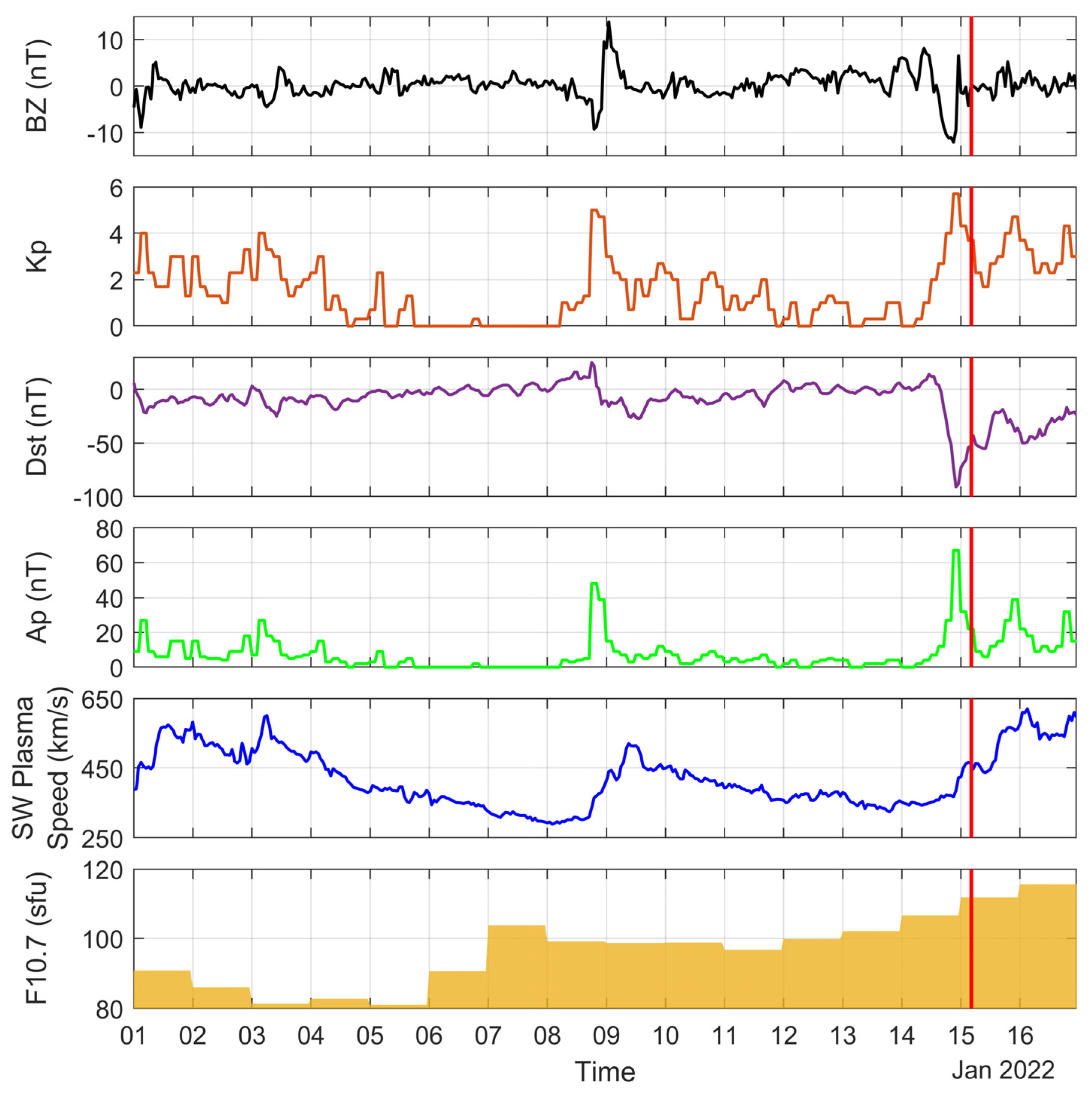
The anomalous variations in the ionosphere are influenced by solar activity and the solar–terrestrial space environment, and the perturbations caused by the space environment are usually widespread [37]. This means that anomalies in ionosphere-related parameters may not only appear in volcanic eruption regions. Therefore, local anomalies near the eruption region may be potentially related to the eruption. When analyzing the abnormal variations in the ionosphere before the volcanic eruption, it is necessary to comprehensively analyze the variations in the space environment during this period to exclude the interference of space environment factors. In this paper, the Bz component of the interplanetary magnetic field (IMF), as well as the Kp index, Dst index, Ap index, solar wind plasma speed and 10.7 cm solar radio flux (F10.7) for a total of 16 days before and after the volcanic eruption are selected as criteria to judge the degree of disturbance in the solar–terrestrial space environment.
2.3. Sliding Interquartile Range
The sliding interquartile range method is widely used in pre-seismic ionospheric TEC anomaly detection, and is similar to the moving average method [6,38]. Compared with the conventional method, it can calculate the background value more accurately, and then calculate the upper and lower limits of ionospheric TEC based on the background value to detect the presence of anomalous values. Using the 20-day data as an example, the data are arranged from smallest to largest as , then
where – are the upper interquartile, median and lower interquartile, respectively. First, a suitable sliding time window is selected and the TEC values under the window are arranged from smallest to largest and divided into four equal parts. The parity line is represented as Equations (1)–(3) in order, and then the interquartile range value is represented as Equation (4).
Since the solar activity cycle is 27 days, this paper uses 27 days as the sliding window to detect the ionospheric TEC perturbation condition before the volcanic eruption. The upper bound of TEC anomaly is represented as and the lower bound as .
2.4. NeuralProphet
Facebook offers an interpretable model called Prophet that can be extended to many predictive applications. The NeuralProphet adds autoregressive and covariate modules on the basis of Prophet. These modules can be configured as classical linear regression or neural networks, and perform better than Prophet on various data sets. The prediction accuracy of NeuralProphet is 55~92% higher than that of Prophet in short-term and medium-term prediction [39].
A core concept of the NeuralProphet model is its modular composability. The model consists of modules, each of which contributes an additional component to the prediction, where h defines the number of steps from one prediction to the future and all modules must produce h outputs. The following equation describes the one-step ahead prediction for h = 1.
where represents the trend term at time t, denotes the seasonal effect at time t, denotes the event and holiday effect at time t, denotes the regression effect of future known exogenous variables at time t, represents the autoregressive effect at time t, and denotes the regression effect of lagged observations of exogenous variables at time t.
In this paper, the value of h is set to 16 days, and the amount of training and testing data is consistent with that of the sliding interquartile range method. The upper and lower bounds of TEC anomalies are expressed in terms of the error in predicting TEC, as follows.
2.5. Wavelet Transform
As a time–frequency localization analysis tool for data, wavelet transform has achieved many achievements in meteorology, astronomy and geophysics [40]. Among them, cross-wavelet transform (XWT) and wavelet coherence (WTC) analysis can better explain the correlation between two time series and in the time–frequency space. It is defined as follows.
where ∗ represents the complex conjugate. is defined as the cross-wavelet power, and and are the background power spectra of and , respectively. The Equation (10) shows the formula for the theoretical distribution of cross-wavelet power, where and are the standard deviations. When the background power spectrum is real wavelet v = 1 and v = 2 when it is complex wavelet, is the confidence level of the probability p.
Wavelet coherence spectrum analysis can reflect the covariance strength of two time series in time–frequency space, covering the correlation in their low-energy regions. It is defined as in Equation (11), where S is the smoothing operator. The significance test of the wavelet coherence spectrum is performed using the Monte Carlo method wavelet coherence value R2 between 0 and 1, and its larger value indicates a stronger correlation.
3. Results
The ionospheric TEC is impacted by solar forcing, geomagnetic forcing and lower atmospheric forcing, and the prerequisite for exploring whether the ionosphere is anomalous before the volcanic eruption presupposes a quiet solar–terrestrial space environment. For this purpose, we obtained the solar wind plasma velocity and F10.7 index, which characterize the intensity of solar activity; the Bz component of the IMF, which characterizes the space environment; and the Kp, Dst and Ap index, which characterize the geomagnetic storm condition, for analysis and exploration. The variations of the indices are shown in Figure 2. We can clearly see that the Bz component exceeds 10 nT, the Kp index is close to 5, the Dst index is close to −30 nT, and the Ap index also exceeds 40 nT on the 8th and 9th from Figure 2, while the space environmental events broadcasted by the Space Environment Prediction Center (SPEC) of the Chinese Academy of Sciences show that geomagnetic storms occurred on these two days. Similarly, a large disturbance occurred in the space environment a few hours before the volcanic eruption. The Bz component was lower than −10 nT, and the Dst index was close to −100 nT, which was a geomagnetic storm.
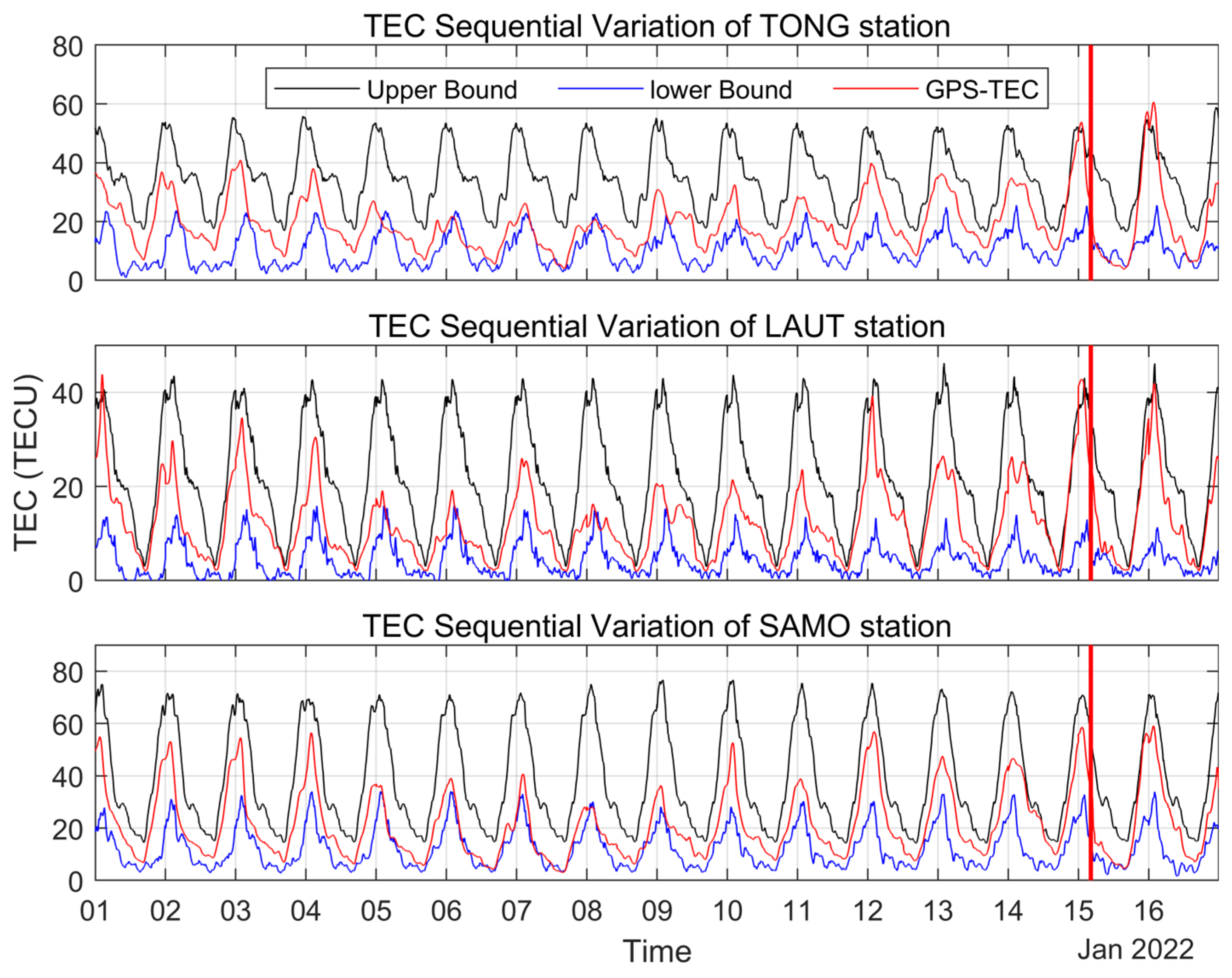
We applied the sliding interquartile range method to detect ionospheric TEC anomalies at TONG, LAUT and SAMO stations near the volcanic eruption, as shown in Figure 3 and Figure 4. The Figure 3 shows the ionospheric TEC variations over the three GNSS stations from 1 to 16 January 2022, where the black line indicates the upper bound of the detected TEC, the blue line indicates the lower bound of the detected TEC, the red line is the variations of the measured TEC, and the red vertical line indicates the moment of volcanic eruption. From the ionospheric TEC values, the values at TONG and LAUT stations are closer, and the TEC over SAMO station is overall higher than those at TONG and LAUT stations. However, the TEC changes at the three stations are consistent, and all show a decrease in TEC peak from 5 January, and this phenomenon continues until 11 January. The ionospheric TEC anomalies detected over the three stations are shown in Figure 4. As shown in Figure 4, the TEC over the three stations exhibited negative anomalies on 5, 6 and 8 January during the 15 days before the eruption. Among them, the negative anomaly on 5 January had the longest duration at TONG station; the maximum anomaly value exceeded 5 TECU at both TONG and SAMO stations, and the peak value of this anomaly was also higher than 2 TECU at LAUT station. On 6 January, negative anomalies of about 5 TECU were also observed at TONG and SAMO stations, but the anomaly at LAUT station was only about 1 TECU and of shorter duration. On 8 January, all three stations showed negative anomalies of about 2 TECU. Positive TEC anomalies were observed over TONG and LAUT stations on the 14th and 15th, with anomalies of about 2 TECU on the 14th and peak values near 5 TECU on the 15th. One day after the eruption, only TONG station showed negative anomalies of about 5 TECU and positive anomalies of more than 10 TECU, and no anomalies were observed at the other two stations. This indicates that the volcanic eruption only caused TEC anomalies at TONG station within a short period of time and failed to affect the distant areas. The ionospheric anomalies during and after the eruption have been studied more and will not be discussed here.
Considering the problem of insufficient support of using only one anomaly detection method, we used NeuralProphet as an additional anomaly detection method and applied the same data to detect the ionospheric TEC anomaly before the volcanic eruption, as shown in Figure 5 and Figure 6. Figure 5 shows the time series of GPS-TEC and that predicted by NeuralProphet over the three stations from 1 to 16 January. It can be seen from Figure 5 that the predicted TEC by NeuralProphet reproduces the trend of GPS-TEC better. The ionospheric TEC anomalies detected using NeuralProphet are given in Figure 6, where the black line indicates the upper bound of the detected TEC anomaly, the blue line indicates the lower bound of the detected TEC anomaly, the orange line shows the change in the predicted TEC error, and the red vertical line indicates the moment of volcanic eruption. As can be seen from Figure 6, the TEC anomalies detected using NeuralProphet are similar to those detected using the sliding interquartile range, with negative TEC anomalies also occurring at three stations on the 5th, 6th and 8th, and positive TEC anomalies on the 14th and 15th. This also indicates that the TEC anomalies detected using both detection methods are more reliable.
Combined with Figure 2, Figure 3, Figure 4, Figure 5 and Figure 6, there was a large harassment to the ionosphere due to the geomagnetic storms on the 8, 9, 14 and 15 January. Although the various geomagnetic indices did not show the occurrence of geomagnetic storms on the 6th, the F10.7 index on the 6th showed a sudden increase of nearly 10 sfu compared to that on the 5th. The Space Environment Prediction Center also showed the occurrence of a C1.1 solar flare on that day.
In order to further eliminate the interference of the solar–terrestrial space environment on the detection of ionospheric anomalies, we applied cross-wavelet transform and the wavelet coherence spectrum to analyze the correlation between TEC over TONG station and six kinds of solar–terrestrial space environment parameters from 1 to 16 January, as shown in Figure 7 and Figure 8, The right color bar in Figure 7 indicates the cross-wavelet power spectral density, and the arrow direction indicates the phase relationship between the two: to the right indicates that the two sequences are in phase, to the left indicates the opposite phase, vertically down indicates that the former sequence is 1/4 cycle change ahead of the latter sequence, and vertically up indicates that the latter sequence is 1/4 cycle change ahead of the former sequence. Figure 7 shows that the ionospheric TEC has the same resonance period as the six solar–terrestrial space environment parameters, and the TEC has the same phase relationship with Kp and Ap. The wavelet coherence spectrum of TEC with other parameters is given in Figure 8, and the right color bar is the wavelet coherence value, characterizing the strength of coherence. Combining Figure 7 and Figure 8, it can be found that TEC on 8, 9, 14 and 15 January are clearly affected by Bz, Kp, Dst, Ap and SW plasma speed, and TEC on 6 January is affected by F10.7. Therefore, in order to ensure the accuracy of the detected anomalies, the ionospheric anomalies on 6, 8, 9, 14 and 15 January are not explored in this paper, and only the ionospheric anomaly on 5 January is studied.
To investigate the global distribution of the ionospheric anomalies on 5 January, we used GIM data with a resolution of 1 h provided by CODE for the analysis. We also used the sliding interquartile range method to detect the ionospheric TEC anomaly for each grid point. The sliding window was also set to 27 days, and the upper and lower TEC bounds were calculated for each grid point on that day to find the anomaly value, and the results are shown in Figure 9. The global distribution of ionospheric anomalies on 5 January can be clearly seen in Figure 9. The negative anomaly of 4 TECU in the ionospheric TEC starts at 02:00 UT, and the anomaly area is located southeast of the volcanic eruption. The value of the Ionospheric TEC anomaly increases from 02:00 to 04:00 UT, and the occurrence area gradually approaches the volcanic eruption location. The negative anomaly value exceeds 6 TECU at 04:00 UT, and the center of the anomaly is close to the volcanic eruption location. Starting from 05:00 UT, the ionospheric TEC anomaly value gradually decreases, and the anomaly area also keeps shrinking centered on the volcanic eruption location, and the anomaly basically disappears by 07:00 UT.
Figure 10 shows the distribution of the global ionospheric TEC on 5 January. As can be seen from Figure 10, the intensity of the EIA is greatest at 00:00 UT, where the northern peak anomaly is higher than the southern peak anomaly by about 5 TECU in value and smaller than the southern peak anomaly in coverage. The difference between the EIA and the north-south peak gradually decreases from 00:00 UT, the maximum value of the EIA decreases by 16 TECU at 04:00 UT, and the difference between the north–south peak decreases to 1 TECU. The difference between the EIA and the north–south peak gradually increases, and the peak of the EIA is far away from the eruption center from 05:00 UT. This trend is more consistent with the variations of TEC anomaly in Figure 9, indicating that the influence of EIA at the eruption location gradually becomes weaker.
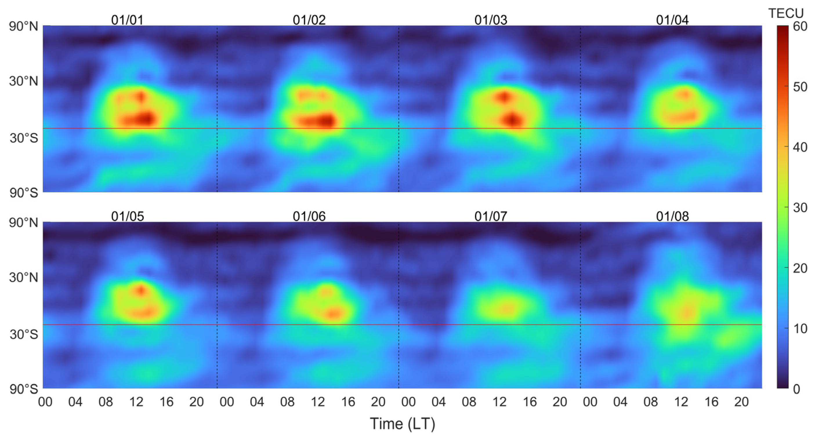
The latitude–time–TEC variation series of the 175°W meridian extracted based on CODE GIM is given in Figure 11 for the period from 1 to 8 January, local time. It can be concluded that the EIA peak shifts significantly toward the Antarctic from 1 to 3 January, appearing from local afternoon to night; the EIA double peak decreases from 4 to 7 January, and the EIA double peak disappears and then merges into a peak on 7 January.
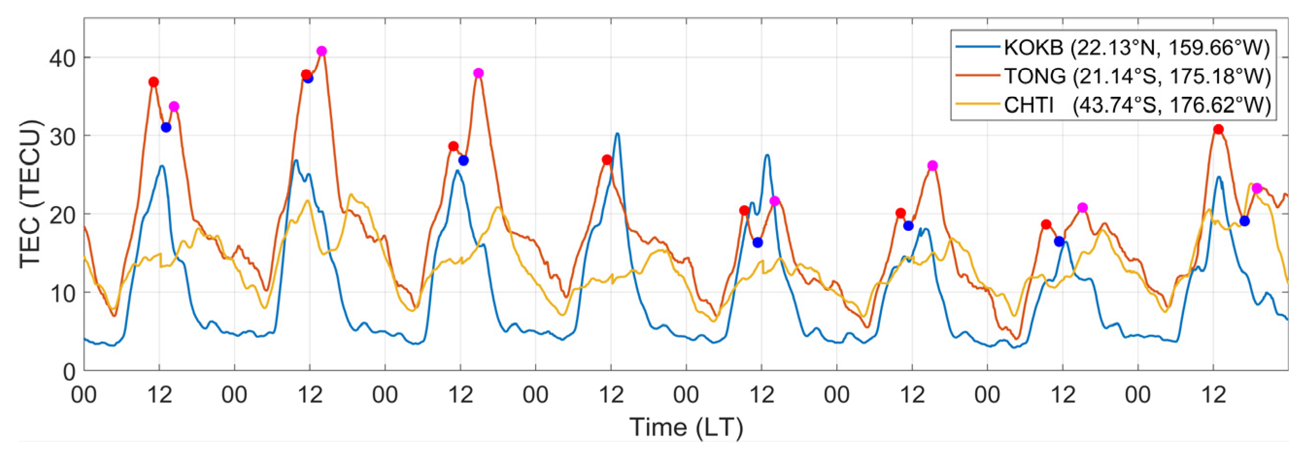
To further investigate the ionospheric TEC anomalies at the same longitude, we selected KOKB and CHTI stations, which are at approximately the same longitude as the TONG station, to analyze their anomalous conditions. Among them, KOKB station is located at the northern peak of the EIA, and CHTI station is located at the mid-latitude of the southern hemisphere, where there is no EIA. Figure 12 shows the TEC time series of KOKB, TONG and CHTI stations from 1 to 8 January (local time). It can be seen from Figure 12 that the diurnal ionospheric TEC variation trends are the same at KOKB and TONG stations, which are located at the EIA peak. However, the daytime TEC variation at CHTI station is more drastic, which may be related to its location. In addition, it is noticeable that the daytime ionospheric peak at TONG station decreases by nearly 10 TECU starting from the 4th day of local time. Interestingly, only one diurnal peak was observed at TONG station on the 4th (5 January UT), while at other times, the ionospheric DDM (also known as the “noontime bite-out”) was observed regardless of the ionospheric TEC values.
Based on the ionospheric electron density data acquired by the FORMOSAT-7/COSMIC-2 occultation, we filtered the data at the location of the time when the ionospheric TEC anomaly occurred in Figure 9 (i.e., 01:30~04:30 UT satellite and GNSS satellite tangent point trajectory close to the volcanic eruption location on 5 January), and obtained a total of eight occultation events for three satellites. Figure 13, Figure 14 and Figure 15 show the ionospheric electron density profiles and tangent point trajectory locations near the eruption. It is clear from Figure 13 that the electron density appears as an extreme value of 7.5 × 10⁵ el/cm3 at 100~130 km altitude (about the E layer of the ionosphere), which also far exceeds the peak in the F2 layer of the ionosphere. This phenomenon is called an ionospheric sporadic E (Es) layer, i.e., a thin layer with significantly larger-than-normal electron density at the height of the E layer by chance, ranging from hundreds to thousands of meters thick, and is a significant anomaly on the E layer. However, this phenomenon does not occur in Figure 14c and Figure 15c.
4. Discussion
In this paper, we detect the TEC anomalies for 16 days before the eruption based on the measured data from three GNSS stations near Tonga volcano, and find inconsistent size anomalies on 5, 6, 8, 9, 14 and 15 January. By analyzing the changes in space weather parameters (Figure 6, Figure 7 and Figure 8), we exclude the ionospheric TEC anomalies on 6, 8, 9, 14 and 15 January. In addition to solar and geomagnetic activity, low atmospheric forcing has the potential to contribute to variations in the ionosphere [41,42]. In order to study the effect of low atmospheric forcing on the ionosphere, we simulated the meridional and zonal winds in the lower atmosphere on 5, 6, 8 and 9 January based on the level of geomagnetic activity using the HWM14 model, as shown in Figure 16. As analyzed above, there was no significant forcing from solar and geomagnetic activities on 5 January, and from 5 to 9 January, there were no significant changes in the meridional and zonal winds, suggesting that low atmospheric forcing did not have an effect on the ionosphere.
The results of the CODE GIM anomaly analysis indicate that the anomaly on 5 January only appeared near the volcanic eruption area and was relatively strong, lasting for about 4 h, while no ionospheric TEC anomalies were observed in other regions of the world during the same period. Liu et al. [43] mentioned in their study of pre-seismic regional ionospheric anomalies that planetary waves and tides usually cause large-scale ionospheric anomalies, and that gravity waves, while they may cause rather small localized features, usually do not last long, and have a single polarity or phase. In this paper, the GIM shows an ionospheric anomaly within a small region of the eruption that lasted 4 h and is unlikely to have been caused by planetary waves and tides or gravity waves.
Since the eruption location is close to the southern peak of the EIA, we studied the EIA of the ionosphere before the eruption (see Figure 11). The analysis results show that the intensity of the EIA double peaks weakened starting on 4 January of local time (i.e., 5 January UT), which is consistent with the GPS-TEC time series results from TONG station in Figure 12. The generator process in the E region during the daytime produces a band electric field in the off-equatorial region, which is mapped to the equatorial F region along the geomagnetic field lines [44], and this electric field pushes the plasma upwards and further diffusion processes and gravity lead to the formation of the EIA [45]. The equatorial E×B electric field and the meridional wind play a decisive role in regulating the strength and position of the EIA [46,47,48,49]. We examined the variations in the neutral component using the globally distributed O/N2 data measured by Global Ultraviolet Imager (GUVI) on the TIMED satellite, as shown in Figure 17. From 5 to 10 January, there is no significant change in the ratio of O/N2 in the eruption region, especially in the latitude region where the EIA occurs, which can be explained by the weakening of the intensity of the EIA on 5 January independently of the change in the neutral component. However, on 9 January, a more significant positive value of O/N2 was observed at 30°N, with 135.6 mm O+ occupying a larger proportion, and it was mentioned above that there was a geomagnetic storm event on 9 January, which may be related to the change of the neutral component, and is beyond the scope of this paper.
The DDM in Figure 12 is caused by the electric field driving the equatorial plasma fountain, moving the plasma to a higher altitude and higher latitude, causing a loss of electron density in the equatorial region around noon. The absence of DDM on 4 January local time is consistent with the cause of the weakening intensity of the EIA wave crest, which may be caused by the electric field drive, and whether it is related to volcanic eruption precursors requires further study.
We find an anomaly phenomenon in the ionospheric E layer on 5 January UT based on electron density data from the FORMOSAT-7/COSMIC-2 occultation, which is particularly notable in Figure 13. It has been shown that the occurrence and spatial and temporal variation of the Es layer are closely related to the wind shear theory, and at low latitudes, especially near the magnetic equator, the wind shear mechanism is not sufficient to form a strong Es layer, and the equatorial Es layer arises from the gradient instability and depends on the electrojet stream [50,51]. This paper alone is not enough to illustrate the relationship between Es layers and volcanic eruption precursors, and we will investigate this phenomenon with more cases in future studies.
5. Conclusions
In this paper, we focus on the anomalous conditions of the ionosphere before the 15 January 2022 eruption of the Tonga volcano. The main results are as follows:
- (1)
- On 5, 6, 8, 9, 14 and 15 January, ionospheric TEC anomalies were detected at TONG, LAUT and SAMO stations, and most of them were negative anomalies. Combining the space weather parameters and applying the cross-wavelet transform and wavelet coherence spectral analysis, we ruled out the effects of solar activity and geomagnetic disturbances. Using the simulated data of neutral winds, we exclude the effect of lower atmospheric forcing. It is tentatively concluded that the negative TEC anomaly detected by the three GNSS stations on 5 January is related to the volcanic eruption.
- (2)
- Based on the CODE GIM data, we apply the sliding interquartile range method to detect a negative anomaly in the global ionospheric TEC on 5 January only near the center of the volcanic eruption, with the maximum anomaly exceeding 6 TECUs, which further confirms that the TEC anomaly on 5 January is closely related to the volcanic eruption.
- (3)
- The sequence of latitude–time–TEC variations along the 175°W meridian shows that the equatorial anomaly wave peaks moved significantly toward the South Pole from the local afternoon to the night from the beginning of the 1st to the 3rd, and the equatorial anomaly double peaks began to decrease from the 4th and disappeared and merged into a single wave by the 7th. The O/N2 data show that the neutral component did not contribute much to the ionospheric variations on the 5 January.
- (4)
- TONG station shows a decrease in the peak of the diurnal ionosphere by nearly 10 TECU from the 4th local time, while only one diurnal peak occurs on the 4th (i.e., 5 January UT), while all other dates of TONG station show a significant ionospheric DDM. Based on the FORMOSAT-7/COSMIC-2 occultation electron density data, we find an Es phenomenon in the ionosphere near the eruption of the volcano on 5 January (UT), with an extreme value of nearly 7.5 × 10⁵ el/cm3 at an altitude of 100–130 km well above the peak of the F2 layer of the ionosphere. Whether these two phenomena are related to the volcanic eruption needs to be explored in depth with more cases.
Author Contributions
Conceptualization, writing—original draft, methodology, J.F., Y.Y. and T.Z.; validation, J.F.; data curation, Y.Y., T.Z., Z.Z. and D.M.; visualization, J.F., Y.Y. and T.Z.; formal analysis, J.F., T.Z., Z.Z. and D.M.; writing—review and editing, J.F., Z.Z. and D.M.; funding acquisition, J.F. All authors have read and agreed to the published version of the manuscript.
Funding
This research was funded by the National Natural Science Foundation of China (Grant No. 42274040) and Project Supported by the Specialized Research Fund for State Key Laboratories.
Data Availability Statement
The GNSS observations are from the IGS (https://cddis.nasa.gov/archive/gnss/data/daily/, regis-tration required, accessed on 30 September 2023). The FORMOSAT-7/COSMIC-2 occultation data are from CDAAC (https://data.cosmic.ucar.edu/gnss-ro/cosmic2/provisional/spaceWeather/, accessed on 30 September 2023). The GIM products are from the CODE Analysis Center (http://ftp.aiub.unibe.ch/CODE/, accessed on 30 September 2023). The wind data are derived from CCMC (https://kauai.ccmc.gsfc.nasa.gov/instantrun/hwm/, accessed on 30 September 2023). The solar geomagnetic parameters are from GSFC/SPDF OMNIWeb (https://omniweb.gsfc.nasa.gov/form/dx4.html, accessed on 30 September 2023), and the O/N2 products are from GUVI (http://guvitimed.jhuapl.edu/, accessed on 30 September 2023).
Acknowledgments
Conflicts of Interest
The authors declare no conflict of interest.
References
- Leonard, R.S.; Barnes, R.A. Observation of ionospheric disturbances following the Alaska earthquake. J. Geophys. Res. 1965, 70, 1250–1253. [Google Scholar] [CrossRef]
- Whitcomb, J.H.; Garmany, J.D.; Anderson, D.L. Earthquake Prediction: Variation of Seismic Velocities before the San Francisco Earthquake. Science 1973, 180, 632–635. [Google Scholar] [CrossRef] [PubMed]
- Pulinets, S. Ionospheric Precursors of Earthquakes; Recent Advances in Theory and Practical Applications. Terr. Atmos. Ocean. Sci. 2004, 15, 413–435. [Google Scholar] [CrossRef]
- Iwata, T.; Umeno, K. Preseismic ionospheric anomalies detected before the 2016 Kumamoto earthquake. J. Geophys. Res. Space Phys. 2017, 122, 3602–3616. [Google Scholar] [CrossRef]
- Xie, T.; Chen, B.; Wu, L.; Dai, W.; Kuang, C.; Miao, Z. Detecting Seismo-Ionospheric Anomalies Possibly Associated with the 2019 Ridgecrest (California) Earthquakes by GNSS, CSES, and Swarm Observations. J. Geophys. Res. Space Phys. 2021, 126, e2020JA028761. [Google Scholar] [CrossRef]
- Ke, F.; Wang, Y.; Wang, X.; Qian, H.; Shi, C. Statistical analysis of seismo-ionospheric anomalies related to Ms > 5.0 earthquakes in China by GPS TEC. J. Seismol. 2016, 20, 137–149. [Google Scholar] [CrossRef]
- Heki, K. Ionospheric electron enhancement preceding the 2011 Tohoku-Oki earthquake. Geophys. Res. Lett. 2011, 38, L17312. [Google Scholar] [CrossRef]
- Le, H.; Liu, J.Y.; Liu, L. A statistical analysis of ionospheric anomalies before 736 M6.0+ earthquakes during 2002–2010. J. Geophys. Res. Space Phys. 2011, 116. [Google Scholar] [CrossRef]
- Dautermann, T.; Calais, E.; Mattioli, G.S. Global Positioning System detection and energy estimation of the ionospheric wave caused by the 13 July 2003 explosion of the Soufrière Hills Volcano, Montserrat. J. Geophys. Res. Solid Earth 2009, 114, B02202. [Google Scholar] [CrossRef]
- Nakashima, Y.; Heki, K.; Takeo, A.; Cahyadi, M.N.; Aditiya, A.; Yoshizawa, K. Atmospheric resonant oscillations by the 2014 eruption of the Kelud volcano, Indonesia, observed with the ionospheric total electron contents and seismic signals. Earth Planet. Sci. Lett. 2016, 434, 112–116. [Google Scholar] [CrossRef]
- Liu, X.; Zhang, Q.; Shah, M.; Hong, Z. Atmospheric-ionospheric disturbances following the April 2015 Calbuco volcano from GPS and OMI observations. Adv. Space Res. 2017, 60, 2836–2846. [Google Scholar] [CrossRef]
- Gonnermann, H.M.; Manga, M. The Fluid Mechanics Inside a Volcano. Annu. Rev. Fluid Mech. 2006, 39, 321–356. [Google Scholar] [CrossRef]
- Astafyeva, E. Ionospheric Detection of Natural Hazards. Rev. Geophys. 2019, 57, 1265–1288. [Google Scholar] [CrossRef]
- Heki, K. Explosion energy of the 2004 eruption of the Asama Volcano, central Japan, inferred from ionospheric disturbances. Geophys. Res. Lett. 2006, 33, L14303. [Google Scholar] [CrossRef]
- Kanamori, H.; Mori, J. Harmonic excitation of mantle Rayleigh waves by the 1991 eruption of Mount Pinatubo, Philippines. Geophys. Res. Lett. 1992, 19, 721–724. [Google Scholar] [CrossRef]
- Kakinami, Y.; Kamogawa, M.; Tanioka, Y.; Watanabe, S.; Gusman, A.R.; Liu, J.-Y.; Watanabe, Y.; Mogi, T. Tsunamigenic ionospheric hole. In Geophysical Research Letters; Wiely: Hoboken, NJ, USA, 2012; Volume 39. [Google Scholar] [CrossRef]
- Shults, K.; Astafyeva, E.; Adourian, S. Ionospheric detection and localization of volcano eruptions on the example of the April 2015 Calbuco events. J. Geophys. Res. Space Phys. 2016, 121, 10303–10315. [Google Scholar] [CrossRef]
- Afraimovich, E.L.; Astafieva, E.I.; Kirushkin, V.V. Localization of the source of ionospheric disturbance generated during an earthquake. Int. J. Geomagn. Aeron. 2006, 6, GI2002. [Google Scholar] [CrossRef]
- Li, J.; Meng, G.; You, X.; Zhang, R.; Shi, H.; Han, Y. Ionospheric total electron content disturbance associated with May 12, 2008, Wenchuan earthquake. Geod. Geodyn. 2015, 6, 126–134. [Google Scholar] [CrossRef]
- Li, W.; Guo, J.; Yue, J.; Shen, Y.; Yang, Y. Total electron content anomalies associated with global VEI4+ volcanic eruptions during 2002–2015. J. Volcanol. Geotherm. Res. 2016, 325, 98–109. [Google Scholar] [CrossRef]
- Zhou, M.; Gao, H.; Yu, D.; Guo, J.; Zhu, L.; Yang, L.; Pan, S. Analysis of the Anomalous Environmental Response to the 2022 Tonga Volcanic Eruption Based on GNSS. Remote Sens. 2022, 14, 4847. [Google Scholar] [CrossRef]
- Harding, B.J.; Wu, Y.-J.J.; Alken, P.; Yamazaki, Y.; Triplett, C.C.; Immel, T.J.; Gasque, L.C.; Mende, S.B.; Xiong, C. Impacts of the January 2022 Tonga Volcanic Eruption on the Ionospheric Dynamo: ICON-MIGHTI and Swarm Observations of Extreme Neutral Winds and Currents. Geophys. Res. Lett. 2022, 49, e2022GL098577. [Google Scholar] [CrossRef]
- Zhang, J.; Xu, J.; Wang, W.; Wang, G.; Ruohoniemi, J.M.; Shinbori, A.; Nishitani, N.; Wang, C.; Deng, X.; Lan, A.; et al. Oscillations of the Ionosphere Caused by the 2022 Tonga Volcanic Eruption Observed With SuperDARN Radars. Geophys. Res. Lett. 2022, 49, e2022GL100555. [Google Scholar] [CrossRef]
- Aa, E.; Zhang, S.-R.; Wang, W.; Erickson, P.J.; Qian, L.; Eastes, R.; Harding, B.J.; Immel, T.J.; Karan, D.K.; Daniell, R.E.; et al. Pronounced Suppression and X-Pattern Merging of Equatorial Ionization Anomalies after the 2022 Tonga Volcano Eruption. J. Geophys. Res. Space Phys. 2022, 127, e2022JA030527. [Google Scholar] [CrossRef] [PubMed]
- Astafyeva, E.; Maletckii, B.; Mikesell, T.D.; Munaibari, E.; Ravanelli, M.; Coisson, P.; Manta, F.; Rolland, L. The 15 January 2022 Hunga Tonga eruption history as inferred from ionospheric observations. Geophys. Res. Lett. 2022, 49, e2022GL098827. [Google Scholar] [CrossRef]
- Lin, J.-T.; Rajesh, P.K.; Lin, C.C.H.; Chou, M.-Y.; Liu, J.-Y.; Yue, J.; Hsiao, T.-Y.; Tsai, H.-F.; Chao, H.-M.; Kung, M.-M. Rapid Conjugate Appearance of the Giant Ionospheric Lamb Wave Signatures in the Northern Hemisphere After Hunga-Tonga Volcano Eruptions. Geophys. Res. Lett. 2022, 49, e2022GL098222. [Google Scholar] [CrossRef]
- Heki, K. Ionospheric signatures of repeated passages of atmospheric waves by the 2022 Jan. 15 Hunga Tonga-Hunga Ha’apai eruption detected by QZSS-TEC observations in Japan. Earth Planets Space 2022, 74, 112. [Google Scholar] [CrossRef]
- Hong, J.; Kil, H.; Lee, W.K.; Kwak, Y.-S.; Choi, B.-K.; Paxton, L.J. Detection of Different Properties of Ionospheric Perturbations in the Vicinity of the Korean Peninsula After the Hunga-Tonga Volcanic Eruption on 15 January 2022. Geophys. Res. Lett. 2022, 49, e2022GL099163. [Google Scholar] [CrossRef]
- Ghent, J.N.; Crowell, B.W. Spectral Characteristics of Ionospheric Disturbances Over the Southwestern Pacific from the 15 January 2022 Tonga Eruption and Tsunami. Geophys. Res. Lett. 2022, 49, e2022GL100145. [Google Scholar] [CrossRef]
- Themens, D.R.; Watson, C.; Žagar, N.; Vasylkevych, S.; Elvidge, S.; McCaffrey, A.; Prikryl, P.; Reid, B.; Wood, A.; Jayachandran, P.T. Global Propagation of Ionospheric Disturbances Associated with the 2022 Tonga Volcanic Eruption. Geophys. Res. Lett. 2022, 49, e2022GL098158. [Google Scholar] [CrossRef]
- Saito, S. Ionospheric disturbances observed over Japan following the eruption of Hunga Tonga-Hunga Ha’apai on 15 January 2022. Earth Planets Space 2022, 74, 57. [Google Scholar] [CrossRef]
- Timoté, C.C.; Juan, J.M.; Sanz, J.; González-Casado, G.; Rovira-García, A.; Escudero, M. Impact of medium-scale traveling ionospheric disturbances on network real-time kinematic services: CATNET study case. J. Space Weather. Space Clim. 2020, 10, 29. [Google Scholar] [CrossRef]
- Yang, Z.; Morton, Y.T.J.; Zakharenkova, I.; Cherniak, I.; Song, S.; Li, W. Global View of Ionospheric Disturbance Impacts on Kinematic GPS Positioning Solutions during the 2015 St. Patrick’s Day Storm. J. Geophys. Res. Space Phys. 2020, 125, e2019JA027681. [Google Scholar] [CrossRef]
- Carter, B.A.; Pradipta, R.; Dao, T.; Currie, J.L.; Choy, S.; Wilkinson, P.J.; Maher, P.S.; Marshall, R.A.; Harima, K.; LeHuy, M.; et al. The ionospheric effects of the 2022 Hunga Tonga Volcano eruption and the associated impacts on GPS Precise Point Positioning across the Australian region. ESS Open Arch. 2023, 21, e2023SW003476. [Google Scholar] [CrossRef]
- Nayir, H.; Arikan, F.; Arikan, O.; Erol, C.B. Total Electron Content Estimation with Reg-Est. J. Geophys. Res. Space Phys. 2007, 112, A11. [Google Scholar] [CrossRef]
- Sezen, U.; Arikan, F.; Arikan, O.; Ugurlu, O.; Sadeghimorad, A. Online, automatic, near-real time estimation of GPS-TEC: IONOLAB-TEC. Space Weather.-Int. J. Res. Appl. 2013, 11, 297–305. [Google Scholar] [CrossRef]
- Tsurutani, B.; Mannucci, A.; Iijima, B.; Abdu, M.A.; Sobral, J.H.A.; Gonzalez, W.; Guarnieri, F.; Tsuda, T.; Saito, A.; Yumoto, K.; et al. Global dayside ionospheric uplift and enhancement associated with interplanetary electric fields. J. Geophys. Res. Space Phys. 2004, 109, A8. [Google Scholar] [CrossRef]
- Pundhir, D.; Singh, B.; Singh, O.P.; Gupta, S.K.; Karia, S.P.; Pathak, K.N. Study of ionospheric precursors using GPS and GIM-TEC data related to earthquakes occurred on 16 April and 24 September, 2013 in Pakistan region. Adv. Space Res. 2017, 60, 1978–1987. [Google Scholar] [CrossRef]
- Triebe, O.; Hewamalage, H.; Pilyugina, P.; Laptev, N.P.; Bergmeir, C.; Rajagopal, R. NeuralProphet: Explainable Forecasting at Scale. arXiv 2021, arXiv:2111.15397. [Google Scholar] [CrossRef]
- Grinsted, A.; Moore, J.C.; Jevrejeva, S. Application of the cross wavelet transform and wavelet coherence to geophysical time series. Nonlin. Process. Geophys. 2004, 11, 561–566. [Google Scholar] [CrossRef]
- Yang, Z.; Gu, S.-Y.; Qin, Y.; Teng, C.-K.-M.; Wei, Y.; Dou, X. Ionospheric Oscillation with Periods of 6–30 Days at Middle Latitudes: A Response to Solar Radiative, Geomagnetic, and Lower Atmospheric Forcing. Remote Sens. 2022, 14, 5895. [Google Scholar] [CrossRef]
- Lei, J.; Huang, F.; Chen, X.; Zhong, J.; Ren, D.; Wang, W.; Yue, X.; Luan, X.; Jia, M.; Dou, X.; et al. Was Magnetic Storm the Only Driver of the Long-Duration Enhancements of Daytime Total Electron Content in the Asian-Australian Sector between 7 and 12 September 2017? J. Geophys. Res. Space Phys. 2018, 123, 3217–3232. [Google Scholar] [CrossRef]
- Liu, J.Y.; Le, H.; Chen, Y.I.; Chen, C.H.; Liu, L.; Wan, W.; Su, Y.Z.; Sun, Y.Y.; Lin, C.H.; Chen, M.Q. Observations and simulations of seismoionospheric GPS total electron content anomalies before the 12 January 2010 M7 Haiti earthquake. J. Geophys. Res. Space Phys. 2011, 116, A4. [Google Scholar] [CrossRef]
- Rishbeth, H. The F-layer dynamo. Planet. Space Sci. 1971, 19, 263–267. [Google Scholar] [CrossRef]
- Martyn, D. Theory of height and ionization density changes at the maximum of a Chapman-like region, taking account of ion production, decay, diffusion and tidal drift. Phys. Ionos. 1955, 254. [Google Scholar]
- Lin, C.H.; Liu, J.Y.; Fang, T.W.; Chang, P.Y.; Tsai, H.F.; Chen, C.H.; Hsiao, C.C. Motions of the equatorial ionization anomaly crests imaged by FORMOSAT-3/COSMIC. Geophys. Res. Lett. 2007, 34, L19101. [Google Scholar] [CrossRef]
- Chen, Y.; Liu, L.; Le, H.; Wan, W.; Zhang, H. Equatorial ionization anomaly in the low-latitude topside ionosphere: Local time evolution and longitudinal difference. J. Geophys. Res. Space Phys. 2016, 121, 7166–7182. [Google Scholar] [CrossRef]
- Aswathy, R.P.; Manju, G.; Sunda, S. The Response Time of Equatorial Ionization Anomaly Crest: A Unique Precursor to the Time of Equatorial Spread F Initiation. J. Geophys. Res. Space Phys. 2018, 123, 5949–5959. [Google Scholar] [CrossRef]
- Cai, X.; Qian, L.; Wang, W.; McInerney, J.M.; Liu, H.-L.; Eastes, R.W. Hemispherically Asymmetric Evolution of Nighttime Ionospheric Equatorial Ionization Anomaly in the American Longitude Sector. J. Geophys. Res. Space Phys. 2022, 127, e2022JA030706. [Google Scholar] [CrossRef]
- Whitehead, J.D. Recent work on mid-latitude and equatorial sporadic-E. J. Atmos. Terr. Phys. 1989, 51, 401–424. [Google Scholar] [CrossRef]
- Tsunoda, R.T. On blanketing sporadic E and polarization effects near the equatorial electrojet. J. Geophys. Res. Space Phys. 2008, 113, A9. [Google Scholar] [CrossRef]
Figure 1.
Location of volcanic eruption in Tonga (red pentagram) and distribution of GNSS stations (black triangle).
Figure 1.
Location of volcanic eruption in Tonga (red pentagram) and distribution of GNSS stations (black triangle).

Figure 2.
Geomagnetic and solar activity before and after the volcanic eruption from 1 to 16 January 2022. The red vertical line indicates the time of volcanic eruption (same below).
Figure 2.
Geomagnetic and solar activity before and after the volcanic eruption from 1 to 16 January 2022. The red vertical line indicates the time of volcanic eruption (same below).

Figure 3.
Variations in ionospheric TEC over TONG, LAUT and SAMO stations from 1 to 16 January 2022.
Figure 3.
Variations in ionospheric TEC over TONG, LAUT and SAMO stations from 1 to 16 January 2022.

Figure 4.
Ionospheric TEC anomalies detected using the sliding interquartile range method over TONG, LAUT and SAMO stations from 1 to 16 January 2022.
Figure 4.
Ionospheric TEC anomalies detected using the sliding interquartile range method over TONG, LAUT and SAMO stations from 1 to 16 January 2022.

Figure 5.
Ionospheric TEC variations (GPS-TEC and NeuralProphet-TEC) over TONG, LAUT and SAMO stations from 1 to 16 January 2022.
Figure 5.
Ionospheric TEC variations (GPS-TEC and NeuralProphet-TEC) over TONG, LAUT and SAMO stations from 1 to 16 January 2022.

Figure 6.
Ionospheric TEC anomalies detected using NeuralProphet over TONG, LAUT and SAMO stations on 1 to 16 January 2022.
Figure 6.
Ionospheric TEC anomalies detected using NeuralProphet over TONG, LAUT and SAMO stations on 1 to 16 January 2022.

Figure 7.
Cross-wavelet transform of TEC time series and spatial weather parameters from 1 to 16 January 2022 at TONG station. The closed area of the thick black line passes the standard red noise test at 95% confidence level, indicating the significance of the period; the cone of influence (COI) area below the thin black solid line is the area of wavelet transform data with large edge effects, and the thick red line indicates the moment of volcanic eruption.

Figure 8.
Wavelet coherence spectrum of TEC time series with space weather parameters at TONG station from 1 to 16 January 2022.
Figure 8.
Wavelet coherence spectrum of TEC time series with space weather parameters at TONG station from 1 to 16 January 2022.

Figure 9.
Distribution of the global ionospheric TEC anomaly on 5 January, from 02:00 to 07:00 UT. The red pentagram representing the location of the eruption center and the black solid line indicating the magnetic equator (same below).
Figure 9.
Distribution of the global ionospheric TEC anomaly on 5 January, from 02:00 to 07:00 UT. The red pentagram representing the location of the eruption center and the black solid line indicating the magnetic equator (same below).

Figure 10.
Distribution of global ionospheric TEC on 5 January, from 00:00 to 05:00 UT.

Figure 11.
Latitude–time–TEC variations extracted along the 175°W longitude line. The red line is the latitudinal position of the eruption.
Figure 11.
Latitude–time–TEC variations extracted along the 175°W longitude line. The red line is the latitudinal position of the eruption.

Figure 12.
TEC time series of KOKB, TONG and CHTI stations from 1 to 8 January (local time), with the 1st peaks, 2nd peaks and valleys of ionospheric DDM indicated by red, magenta and blue dots, respectively.
Figure 12.
TEC time series of KOKB, TONG and CHTI stations from 1 to 8 January (local time), with the 1st peaks, 2nd peaks and valleys of ionospheric DDM indicated by red, magenta and blue dots, respectively.

Figure 13.
(a) Ionospheric electron density profile near the volcanic eruption detected by FOR-MOSAT-7/COSMIC-2 1st satellite on 5 January. The red pentagram is the location of the eruption, and the line segment in (b) is the tangent point trajectory of the satellite with GNSS satellite.
Figure 13.
(a) Ionospheric electron density profile near the volcanic eruption detected by FOR-MOSAT-7/COSMIC-2 1st satellite on 5 January. The red pentagram is the location of the eruption, and the line segment in (b) is the tangent point trajectory of the satellite with GNSS satellite.

Figure 14.
(a) Ionospheric electron density profile near the volcanic eruption detected by FOR-MOSAT-7/COSMIC-2 2nd satellite on 5 January. The red pentagram is the location of the eruption, and the line segment in (b) is the tangent point trajectory of the satellite with GNSS satellite. Ionospheric electron density profile from 90 to 150 km is shown in (c).

Figure 15.
(a) Ionospheric electron density profile near the volcanic eruption detected by FOR-MOSAT-7/COSMIC-2 4th satellite on 5 January. The red pentagram is the location of the eruption, and the line segment in (b) is the tangent point trajectory of the satellite with GNSS satellite. Ionospheric electron density profile from 90 to 150 km is shown in (c).

Figure 16.
Neutral wind variations from 50 to 100 km above eruption simulated by the HWM14 model during 5–10 January 2022.
Figure 16.
Neutral wind variations from 50 to 100 km above eruption simulated by the HWM14 model during 5–10 January 2022.

Figure 17.
The global distribution of Global Ultraviolet Imager (GUVI)-measured O/N2 ratio during 5–10 January 2022.
Figure 17.
The global distribution of Global Ultraviolet Imager (GUVI)-measured O/N2 ratio during 5–10 January 2022.

Disclaimer/Publisher’s Note: The statements, opinions and data contained in all publications are solely those of the individual author(s) and contributor(s) and not of MDPI and/or the editor(s). MDPI and/or the editor(s) disclaim responsibility for any injury to people or property resulting from any ideas, methods, instructions or products referred to in the content. |
© 2023 by the authors. Licensee MDPI, Basel, Switzerland. This article is an open access article distributed under the terms and conditions of the Creative Commons Attribution (CC BY) license (https://creativecommons.org/licenses/by/4.0/).
Share and Cite
MDPI and ACS Style
Feng, J.; Yuan, Y.; Zhang, T.; Zhang, Z.; Meng, D. Analysis of Ionospheric Anomalies before the Tonga Volcanic Eruption on 15 January 2022. Remote Sens. 2023, 15, 4879. https://doi.org/10.3390/rs15194879
AMA Style
Feng J, Yuan Y, Zhang T, Zhang Z, Meng D. Analysis of Ionospheric Anomalies before the Tonga Volcanic Eruption on 15 January 2022. Remote Sensing. 2023; 15(19):4879. https://doi.org/10.3390/rs15194879
Chicago/Turabian StyleFeng, Jiandi, Yunbin Yuan, Ting Zhang, Zhihao Zhang, and Di Meng. 2023. "Analysis of Ionospheric Anomalies before the Tonga Volcanic Eruption on 15 January 2022" Remote Sensing 15, no. 19: 4879. https://doi.org/10.3390/rs15194879
Note that from the first issue of 2016, this journal uses article numbers instead of page numbers. See further details here.