
Semi-Supervised Learning Method for the Augmentation of an Incomplete Image-Based Inventory of Earthquake-Induced Soil Liquefaction Surface Effects

 , , , and
Abstract
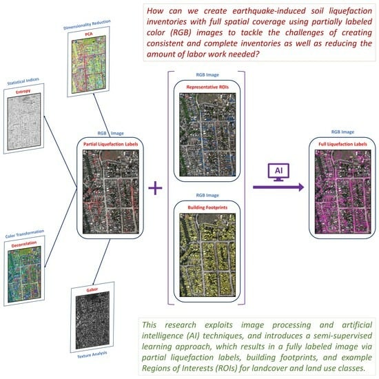
:
1. Introduction
2. Data and Methods
2.1. Datasets
2.1.1. Region of Study
2.1.2. Imagery
2.1.3. Liquefaction Labels
2.1.4. Building Footprints
2.1.5. Land Use and Land Cover ROIs
2.2. Methodology
2.2.1. Fuzzy C-Means Clustering of Liquefaction Data
2.2.2. Feature Extraction from RGB Image

| Category | No. | Feature | Bands | Description | Reference | |
|---|---|---|---|---|---|---|
| Color Image | 1 | RGB | 3 | Red-Blue-Green components of the visible spectrum | [41] | |
| Color Transformations | 2 | HSV | 3 | Saturation (chroma)—the intensity or purity of a hue Brightness (value)—the relative degree of black or white mixed with a given hue Hue—another word for color | [48] | |
| 3 | Decorrelation Stretch | 3 | A linear, pixel-wise operation for visual enhancement Output = T × (Input − mean) + mean T = Transformation Matrix (Covariance-derived) | [49] | ||
| 4 | CMYK | 4 | C, M, Y, and K represent the Cyan, Magenta, Yellow and Black components of the CMYK color space image. | [50] | ||
| Dimensionality Reduction | 5 | Grayscale | 1 | Single-band derivation of the RGB channels Grayscale = (0.2898 × R) + (0.5870 × G) + (0.1140 × B) | [51] | |
| 6 | PCA | 3 | The three variance-based principal components derived from RGB | [52] | ||
| 7 | MNF | 3 | Minimum Noise Fraction rotation transforms are used to determine the inherent dimensionality of image data, to segregate noise in the data, and to reduce the computational requirements for processing. | [53] | ||
| Texture Analysis | 8 | Gabor Filter | 4 | A filter bank representing a linear Gabor filter that is sensitive to textures with a specified wavelength and orientation. | [54] | |
| 9 | Wavelet Transform | 1 | Single-level discrete 2-D wavelet transform derived by taking the tensor products of the one-dimensional wavelet and scaling functions, leading to decomposition of 4 components. The approximation coefficients are used as a single band. | [55] | ||
| 10 | Convolution Filter | 1 | convolution is used to apply filters to an image. A filter (kernel function) is a small matrix of numbers, which is slid over an image, performing a mathematical operation at each position to create a new filtered output image. | [56] | ||
| 11 | Correlation Filter | 1 | GLCM-derived Correlation as a measure of how correlated a pixel is to its neighbor over the whole image. Range = [−1, 1] | [57] | ||
| Statistical Indices | Local Spatial Statistics | 12 | Entropy | 1 | Local entropy of grayscale image (Intensity). Entropy is a statistical measure of Randomness | [56] |
| 13 | Gradient Weight | 1 | Calculates pixel weight for each pixel in the image based on the gradient magnitude at that pixel and returns the weight array. The weight of a pixel is inversely related to the gradient values at the pixel. | [56] | ||
| 14 | Std. Deviation Filter | 1 | Local standard deviation of the image pixels | - | ||
| 15 | Range Filter | 1 | Local range of image pixels (Min–Max) | - | ||
| Pixel Statistics | 16 | Mean Abs. Deviation | 1 | Pixel-based mean absolute deviation of the color bands | - | |
| 17 | Variance | 1 | Pixel-based variance of the color bands | - | ||
| 18 | Sum of Squares | 1 | Pixel-based sum of squares of the color bands | - | ||
| Total number of indices (excluding RGB) = 17 Total number of bands (excluding RGB) = 31 | ||||||
2.2.3. Feature Ranking and Selection
2.2.4. Semi-Supervised Self-Training Classification via Linear Discriminant Analysis
2.2.5. Model Evaluation and Comparative Analysis
3. Results
3.1. Training Data
3.2. Feature Extraction and Ranking
3.3. Semi-Supervised Classification
3.4. Liquefaction Map Visualization
4. Application and Discussion
5. Conclusions
Author Contributions
Funding
Data Availability Statement
Acknowledgments
Conflicts of Interest
References
- van Ballegooy, S.; Malan, P.; Lacrosse, V.; Jacka, M.E.; Cubrinovski, M.; Bray, J.D.; O’Rourke, T.D.; Crawford, S.A.; Cowan, H. Assessment of liquefaction-induced land damage for residential Christchurch. Earthq. Spectra 2014, 30, 31–55. [Google Scholar] [CrossRef]
- Zhu, J.; Daley, D.; Baise, L.G.; Thompson, E.M.; Wald, D.J.; Knudsen, K.L. A geospatial liquefaction model for rapid response and loss estimation. Earthq. Spectra 2015, 31, 1813–1837. [Google Scholar] [CrossRef]
- Meisina, C.; Bonì, R.; Bozzoni, F.; Conca, D.; Perotti, C.; Persichillo, P.; Lai, C.G. Mapping soil liquefaction susceptibility across Europe using the analytic hierarchy process. Bull Earthq. Eng. 2022, 20, 5601–5632. [Google Scholar] [CrossRef]
- Brandenberg, S.J.; Zimmaro, P.; Stewart, J.P.; Kwak, D.Y.; Franke, K.W.; Moss, R.E.; Çetin, K.; Can, G.; Ilgac, M.; Stamatakos, J.; et al. Next-generation liquefaction database. Earthq. Spectra 2020, 36, 939–959. [Google Scholar] [CrossRef]
- Stewart, J.P.; Brandenberg, S.J.; Wang, P.; Nweke, C.C.; Hudson, K.S.; Mazzoni, S.; Bozorgnia, Y.; Hudnut, K.W.; Davis, C.A.; Ahdi, S.K.; et al. (Eds.) Preliminary Report on Engineering and Geological Effects of the July 2019 Ridgecrest Earthquake Sequence; Geotechnical Extreme Events Reconnaissance Association: Berkeley, CA, USA, 2019; Rept. GEER-064. [Google Scholar] [CrossRef]
- Zimmaro, P.; Nweke, C.C.; Hernandez, J.L.; Hudson, K.S.; Hudson, M.B.; Ahdi, S.K.; Boggs, M.L.; Davis, C.A.; Goulet, C.A.; Brandenberg, S.J.; et al. Liquefaction and Related Ground Failure from July 2019 Ridgecrest Earthquake Sequence. Bull. Seismol. Soc. Am. 2020, 110, 1549–1566. [Google Scholar] [CrossRef]
- Ponti, D.J.; Blair, J.L.; Rosa, C.M.; Thomas, K.; Pickering, A.J.; Akciz, S.; Angster, S.; Avouac, J.-P.; Bachhuber, J.; Bacon, S.; et al. Documentation of surface fault rupture and ground deformation features produced by the Ridgecrest M 6.4 and M 7.1 earthquake sequence of July 4 and 5, 2019. Seismol. Res. Lett. 2020, 91, 2942–2959. [Google Scholar] [CrossRef]
- Allstadt, K.E.; Thompson, E.M. Inventory of Liquefaction Features Triggered by the January 7 2020 M6.4 Puerto Rico Earthquake: U.S. Geological Survey Data Release; USGS: Reston, VA, USA, 2021. [CrossRef]
- Rashidian, V.; Baise, L.G.; Koch, M. Using High Resolution Optical Imagery to Detect Earthquake-Induced Liquefaction: The 2011 Christchurch Earthquake. Remote Sens. 2020, 12, 377. [Google Scholar] [CrossRef]
- Zhu, J.; Baise, L.G.; Thompson, E.M. An Updated Geospatial Liquefaction Model for Global Application. Bull. Seismol. Soc. Am. 2017, 107, 1365–1385. [Google Scholar] [CrossRef]
- Sharifi-Mood, M.; Gillins, D.T.; Franke, K.W.; Harper, J.N.; Bartlett, S.J.; Olsen, M.J. Probabilistic liquefaction-induced lateral spread hazard mapping and its application to Utah County, Utah. Eng. Geol. 2018, 237, 76–91. [Google Scholar] [CrossRef]
- Kajihara, K.; Mohan, P.R.; Kiyota, T.; Konagai, K. Liquefaction-induced ground subsidence extracted from Digital Surface Models and its application to hazard map of Urayasu city, Japan. Jpn. Geotech. Soc. Spec. Publ. 2015, 2, 829–834. [Google Scholar] [CrossRef]
- Rathje, E.M.; Franke, K. Remote sensing for geotechnical earthquake reconnaissance. Soil Dyn. Earthq. Eng. 2016, 91, 304–316. [Google Scholar] [CrossRef]
- Ghosh, S.; Huyck, C.K.; Greene, M.; Gill, S.P.; Bevington, J.; Svekla, W.; DesRoches, R.; Eguchi, R.T. Crowdsourcing for rapid damage assessment: The global earth observation catastrophe assessment network (GEO-CAN). Earthq. Spectra 2011, 27, S179–S198. [Google Scholar] [CrossRef]
- Rollins, K.; Ledezma, C.; Montalva, G. (Eds.) Geotechnical Aspects of April 1, 2014, M8.2 Iquique, Chile Earthquake, a Report of the NSF-Sponsored GEER Association Team. GEER Assoc. Report No. GEER-038. 2014. Available online: https://geerassociation.org/components/com_geer_reports/geerfiles/Iquique_Chile_GEER_Report.pdf (accessed on 1 August 2023).
- Hamada, M.; Towhata, I.; Yasuda, S.; Isoyama, R. Study on permanent ground displacement induced by seismic liquefaction. Comput. Geotech. 1987, 4, 197–220. [Google Scholar] [CrossRef]
- Ramakrishnan, D.; Mohanty, K.K.; Natak, S.R.; Vinu Chandran, R. Mapping the liquefaction induced soil moisture changes using remote sensing technique: An attempt to map the earthquake induced liquefaction around Bhuj, Gujarat, India. Geotech. Geol. Eng. 2006, 24, 1581–1602. [Google Scholar] [CrossRef]
- Sengar, S.S.; Kumar, A.; Ghosh, S.K.; Wason, H.R. SOFT COMPUTING APPROACH FOR LIQUEFACTION IDENTIFICATION USING LANDSAT-7 TEMPORAL INDICES DATA. Int. Arch. Photogramm. Remote Sens. Spatial Inf. Sci. 2012, XXXIX-B8, 61–64. [Google Scholar] [CrossRef]
- Oommen, T.; Baise, L.G.; Gens, R.; Prakash, A.; Gupta, R.P. Documenting earthquake-induced liquefaction using satellite remote sensing image transformations. Environ. Eng. Geosci. 2013, 19, 303–318. [Google Scholar] [CrossRef]
- Morgenroth, J.; Hughes, M.W.; Cubrinovski, M. Object-based image analysis for mapping earthquake-induced liquefaction ejecta in Christchurch, New Zealand. Nat. Hazards 2016, 82, 763–775. [Google Scholar] [CrossRef]
- Baik, H.; Son, Y.-S.; Kim, K.-E. Detection of Liquefaction Phenomena from the 2017 Pohang (Korea) Earthquake Using Remote Sensing Data. Remote Sens. 2019, 11, 2184. [Google Scholar] [CrossRef]
- Saraf, A.K.; Sinvhal, A.; Sinvhal, H.; Ghosh, P.; Sarma, B. Liquefaction identification using class-based sensor independent approach based on single pixel classification after 2001 Bhuj, India earthquake. J. Appl. Remote Sens. 2012, 6, 063531. [Google Scholar] [CrossRef]
- Ishitsuka, K.; Tsuji, T.; Matsuoka, T. Detection and mapping of soil liquefaction in the 2011 Tohoku earthquake using SAR interferometry. Earth Planets Space 2012, 64, 1267–1276. [Google Scholar] [CrossRef]
- Bi, C.; Fu, B.; Chen, J.; Zhao, Y.; Yang, L.; Duan, Y.; Shi, Y. Machine learning based fast multi-layer liquefaction disaster assessment. World Wide Web 2019, 22, 1935–1950. [Google Scholar] [CrossRef]
- Njock, P.G.A.; Shen, S.-L.; Zhou, A.; Lyu, H.-M. Evaluation of soil liquefaction using AI technology incorporating a coupled ENN/t-SNE model. Soil Dyn. Earthq Eng. 2020, 130, 105988. [Google Scholar] [CrossRef]
- Hacıefendioğlu, K.; Başağa, H.B.; Demir, G. Automatic detection of earthquake-induced ground failure effects through Faster R-CNN deep learning-based object detection using satellite images. Nat. Hazards 2021, 105, 383–403. [Google Scholar] [CrossRef]
- Zhang, W.; Ghahari, F.; Arduino, P.; Taciroglu, E. A deep learning approach for rapid detection of soil liquefaction using time–frequency images. Soil Dyn. Earthq. Eng. 2023, 166, 107788. [Google Scholar] [CrossRef]
- Feng, Z.; Zhou, Q.; Gu, Q.; Tan, X.; Cheng, G.; Lu, X.; Shi, J.; Ma, L. Dmt: Dynamic mutual training for semi-supervised learning. Pattern Recognit. 2022, 130, 108777. [Google Scholar] [CrossRef]
- Wu, D.; Luo, X.; Wang, G.; Shang, M.; Yuan, Y.; Yan, H. A highly accurate framework for self-labeled semi-supervised classification in industrial applications. IEEE Trans. Ind. Inform. 2017, 14, 909–920. [Google Scholar] [CrossRef]
- Chen, R.; Ma, Y.; Liu, L.; Chen, N.; Cui, Z.; Wei, G.; Wang, W. Semi-supervised anatomical landmark detection via shape-regulated self-training. Neurocomputing 2022, 471, 335–345. [Google Scholar] [CrossRef]
- Oludare, V.; Kezebou, L.; Panetta, K.; Agaian, S.S. Semi-supervised learning for improved post-disaster damage assessment from satellite imagery. Multimodal Image Exploitation and Learning 2021 2021, 1734, 172–182. [Google Scholar] [CrossRef]
- Abdelkader, E.M. On the hybridization of pre-trained deep learning and differential evolution algorithms for semantic crack detection and recognition in ensemble of infrastructures, Smart and Sustain. Built Environ. 2021, 11, 740–764. [Google Scholar] [CrossRef]
- Nhat-Duc, H.; Van-Duc, T. Computer Vision-Based Severity Classification of Asphalt Pavement Raveling Using Advanced Gradient Boosting Machines and Lightweight Texture Descriptors. Iran J. Sci. Technol. Trans. Civ. Eng. 2023. [Google Scholar] [CrossRef]
- Dumitru, C.O.; Cui, S.; Faur, D.; Datcu, M. Data Analytics for Rapid Mapping: Case Study of a Flooding Event in Germany and the Tsunami in Japan Using Very High-Resolution SAR Images. IEEE J. Sel. Top. Appl. Earth Obs. Remote Sens. 2015, 8, 114–129. [Google Scholar] [CrossRef]
- Chatterjee, S. Vision-based rock-type classification of limestone using multi-class support vector machine. Appl. Intell. 2013, 39, 14–27. [Google Scholar] [CrossRef]
- Kumar, C.; Chatterjee, S.; Oommen, T.; Guha, A. Multi-sensor datasets-based optimal integration of spectral, textural, and morphological characteristics of rocks for lithological classification using machine learning models. Geocarto Int. 2021, 37, 6004–6032. [Google Scholar] [CrossRef]
- Cubrinovski, M.; Bray, J.D.; Taylor, M.; Giorgini, S.; Bradley, B.A.; Wotherspoon, L.; Zupan, J. Soil liquefaction effects in the central business district during the February 2011 Christchurch Earthquake. Seismol Res. Lett. 2011, 82, 893–904. [Google Scholar] [CrossRef]
- Geyin, M.; Maurer, B.W.; Bradley, B.A.; Green, R.A.; van Ballegooy, S. CPT-based liquefaction case histories compiled from three earthquakes in Canterbury, New Zealand. Earthq. Spectra 2021, 37, 2920–2945. [Google Scholar] [CrossRef]
- Green, R.A.; Cubrinovski, M.; Cox, B.; Wood, C.; Wotherspoon, L.; Bradley, B.; Maurer, B. Select Liquefaction Case Histories from the 2010–2011 Canterbury Earthquake Sequence. Earthq. Spectra 2014, 30, 131–153. [Google Scholar] [CrossRef]
- Orense, R.P.; Nathan, A.H.; Brian, T.H.; Michael, J.P. Spatial evaluation of liquefaction potential in Christchurch following the 2010/2011 Canterbury earthquakes. Int. J. Geotech. Eng. 2014, 8, 420–425. [Google Scholar] [CrossRef]
- LINZ. Christchurch Post-Earthquake 0.1m Urban Aerial Photos (24 February 2011), Land Information New Zealand (LINZ). 2011. Available online: https://data.linz.govt.nz/layer/51932-christchurch-post-earthquake-01m-urban-aerial-photos-24-february-2011 (accessed on 1 August 2023).
- Townsend, D.; Lee, J.M.; Strong, D.T.; Jongens, R.; Lyttle, B.S.; Ashraf, S.; Rosser, B.; Perrin, N.; Lyttle, K.; Cubrinovski, M.; et al. Mapping surface liquefaction caused by the September 2010 and February 2011 Canterbury earthquakes: A digital dataset. N. Z. J. Geol. Geophys. 2016, 59, 496–513. [Google Scholar] [CrossRef]
- Sanon, C.; Laurie, G.B.; Asadi, A.; Koch, M.; Aimaiti, Y.; Moaveni, B. A Feature-based Liquefaction Image Dataset for Assessing Liquefaction Extent and Impact. In Proceedings of the 2022 Annual Meeting of the Seismological Society of America (SSA), Bellevue, WA, USA, 19–23 October 2022. [Google Scholar]
- Land Information New Zealand (LINZ). 2011. Available online: https://data.linz.govt.nz/layer/101292-nz-building-outlines-all-sources (accessed on 1 August 2023).
- Bezdek, J.C. Pattern Recognition with Fuzzy Objective Function Algorithms; Springer: Boston, MA, USA, 1981. [Google Scholar] [CrossRef]
- Gnädinger, F.; Schmidhalter, U. Digital Counts of Maize Plants by Unmanned Aerial Vehicles (UAVs). Remote Sens. 2017, 9, 544. [Google Scholar] [CrossRef]
- Khorrami, R.A.; Naeimi, Z.; Wing, M.; Ahani, H.; Bateni, S.M. A New Multistep Approach to Identify Leaf-Off Poplar Plantations Using Airborne Imagery. J. Geogr. Inf. Syst. 2022, 14, 634–651. [Google Scholar] [CrossRef]
- Smith, A.R. Color Gamut Transform Pairs. In Proceedings of the SIGGRAPH 78 Conference Proceedings, New York, NY, USA, 23–25 August 1978; pp. 12–19. [Google Scholar]
- CHAPTER 12—Sparsity in Redundant Dictionaries. In A Wavelet Tour of Signal Processing, 3rd ed.; Stéphane, M. (Ed.) Academic Press: Cambridge, MA, USA, 2009; pp. 611–698. ISBN 9780123743701. [Google Scholar] [CrossRef]
- Kang, H.R. Digital Color Halftoning; SPIE Press: Bellingham, WA, USA, 1999; p. 1. ISBN 0-8194-3318-7. [Google Scholar]
- Burger, W.; Mark, J.B. Principles of Digital Image Processing Core Algorithms; Science & Business Media; Springer: Berlin/Heidelberg, Germany, 2010; pp. 110–111. ISBN 978-1-84800-195-4. [Google Scholar]
- Jolliffe, I.T. Principal Component Analysis, 2nd ed.; Springer: Berlin/Heidelberg, Germany, 2002. [Google Scholar]
- Boardman, J.W.; Kruse, F.A. Automated Spectral Analysis: A Geological Example Using AVIRIS Data, North Grapevine Mountains, Nevada. In Proceedings of the ERIM Tenth Thematic Conference on Geologic Remote Sensing, Environmental Research Institute of Michigan, Ann Arbor, MI, USA, 1 January 1994; pp. I-407–I-418. [Google Scholar]
- Jain, A.K.; Farrokhnia, F. Unsupervised Texture Segmentation Using Gabor Filters. Pattern Recognit. 1991, 24, 1167–1186. [Google Scholar] [CrossRef]
- Meyer, Y. Wavelets and Operators; Salinger, D.H., Translator; Cambridge University Press: Cambridge, UK, 1995. [Google Scholar]
- Gonzalez, R.C.; Woods, R.E.; Eddins, S.L. Digital Image Processing Using MATLAB; Chapter 11; Dorling Kindersley Pvt Ltd.: Prentice Hall, NJ, USA, 2003. [Google Scholar]
- Haralick, R.M.; Shanmugan, K.; Dinstein, I. Textural Features for Image Classification. IEEE Trans. Syst. Man Cybern. 1973, SMC-3, 610–621. [Google Scholar] [CrossRef]
- Rojas, R. Neural Networks: A Systematic Introduction; Springer: Berlin/Heidelberg, Germany, 1996. [Google Scholar] [CrossRef]
- Ding, C.; Peng, H. Minimum redundancy feature selection from microarray gene expression data. J. Bioinform. Comput. Biol. 2005, 3, 185–205. [Google Scholar] [CrossRef] [PubMed]
- Darbellay, G.A.; Vajda, I. Estimation of the information by an adaptive partitioning of the observation space. IEEE Trans. Inf. Theory. 1999, 45, 1315–1321. [Google Scholar] [CrossRef]
- Fisher, R.A. The Use of Multiple Measurements in Taxonomic Problems. Ann. Eugen. 1936, 7, 179–188. [Google Scholar] [CrossRef]
- Guo, Y.; Hastie, T.; Tibshirani, R. Regularized linear discriminant analysis and its application in microarrays. Biostatistics 2007, 8, 86–100. [Google Scholar] [CrossRef]
- Papathanassiou, G.; Pavlides, S.; Christaras, B.; Pitilakis, K. Liquefaction case histories and empirical relations of earthquake magnitude versus distance from the broader Aegean region. J. Geodyn. 2005, 40, 257–278. [Google Scholar] [CrossRef]
- Karastathis, V.K.; Karmis, P.; Novikova, T.; Roumelioti, Z.; Gerolymatou, E.; Papanastassiou, D.; Liakopoulos, S.; Tsombos, P.; Papadopoulos, G.A. The contribution of geophysical techniques to site characterisation and liquefaction risk assessment: Case study of Nafplion City, Greece. J. Appl. Geophys. 2010, 72, 194–211. [Google Scholar] [CrossRef]


| Area Coverage | Model Evaluation Tile | Model Application Tile | |
|---|---|---|---|
| Sanon et al. (2022) [43] | Validation Label | Sanon et al. (2022) [43] | |
| Total Extent (m2) | ~9919 | ~44,513 | ~38,500 |
| Percentage of Tile | 2.87% | 12.88% | 11.14% |
| Feature Category | No. | Feature Description | Score | Rank | Selection |
|---|---|---|---|---|---|
| Color Transformation | 1 | Black (CMYK) | 0.791 | 1 |  |
| 2 | Magenta (CMYK) | 0.675 | 2 | | |
| 3 | Cyan (CMYK) | 0.652 | 3 | - | |
| 4 | Decorrelation Stretch (Band 1) | 0.409 | 4 | - | |
| 5 | Hue (HSV) | 0.404 | 5 | - | |
| 6 | Value (HSV) | 0.387 | 6 | - | |
| 7 | Decorrelation Stretch (Band 3) | 0.386 | 7 | - | |
| 8 | Saturation (HSV) | 0.304 | 8 | - | |
| 9 | Yellow (CMYK) | 0.271 | 9 | - | |
| 10 | Decorrelation Stretch (Band 2) | 0.198 | 10 | - | |
| Texture Analysis | 11 | Approximation Coefficients (WT) | 0.794 | 1 | |
| 12 | Gabor Filters (45 deg) | 0.232 | 2 | - | |
| 13 | Gabor Filters (135 deg) | 0.229 | 3 | - | |
| 14 | Gabor Filters (90 deg) | 0.215 | 4 | - | |
| 15 | Convolution Filter | 0.193 | 5 | - | |
| 16 | Gabor Filters (180 deg) | 0.185 | 6 | - | |
| 17 | Correlation Filter | 0.048 | 7 | - | |
| Statistical Indices | 18 | Sum of Squares | 0.813 | 1 | |
| 19 | Gradient Weight | 0.573 | 2 | | |
| 20 | Pixel Variance | 0.561 | 3 | - | |
| 21 | Range Filter | 0.553 | 4 | - | |
| 22 | Entropy Filter | 0.551 | 5 | - | |
| 23 | Mean Absolute Deviation | 0.412 | 6 | - | |
| 24 | Standard Deviation Filter | 0.158 | 7 | - | |
| Dimensionality Reduction | 25 | PCA (Band 1) | 0.818 | 1 | |
| 26 | PCA (Band 2) | 0.646 | 2 | | |
| 27 | MNF (Band 2) | 0.364 | 3 | - | |
| 28 | Grayscale Image | 0.260 | 4 | - | |
| 29 | MNF (Band 1) | 0.187 | 5 | - | |
| 30 | PCA (Band 3) | 0.103 | 6 | - | |
| 31 | MNF (Band 3) | 0.079 | 7 | - |
Disclaimer/Publisher’s Note: The statements, opinions and data contained in all publications are solely those of the individual author(s) and contributor(s) and not of MDPI and/or the editor(s). MDPI and/or the editor(s) disclaim responsibility for any injury to people or property resulting from any ideas, methods, instructions or products referred to in the content. |
© 2023 by the authors. Licensee MDPI, Basel, Switzerland. This article is an open access article distributed under the terms and conditions of the Creative Commons Attribution (CC BY) license (https://creativecommons.org/licenses/by/4.0/).
Share and Cite
Asadi, A.; Baise, L.G.; Sanon, C.; Koch, M.; Chatterjee, S.; Moaveni, B. Semi-Supervised Learning Method for the Augmentation of an Incomplete Image-Based Inventory of Earthquake-Induced Soil Liquefaction Surface Effects. Remote Sens. 2023, 15, 4883. https://doi.org/10.3390/rs15194883
Asadi A, Baise LG, Sanon C, Koch M, Chatterjee S, Moaveni B. Semi-Supervised Learning Method for the Augmentation of an Incomplete Image-Based Inventory of Earthquake-Induced Soil Liquefaction Surface Effects. Remote Sensing. 2023; 15(19):4883. https://doi.org/10.3390/rs15194883
Chicago/Turabian StyleAsadi, Adel, Laurie Gaskins Baise, Christina Sanon, Magaly Koch, Snehamoy Chatterjee, and Babak Moaveni. 2023. "Semi-Supervised Learning Method for the Augmentation of an Incomplete Image-Based Inventory of Earthquake-Induced Soil Liquefaction Surface Effects" Remote Sensing 15, no. 19: 4883. https://doi.org/10.3390/rs15194883