Fast Tailings Pond Mapping Exploiting Large Scene Remote Sensing Images by Coupling Scene Classification and Sematic Segmentation Models

Abstract

In the process of extracting tailings ponds from large scene remote sensing images, semantic segmentation models usually perform calculations on all small-size remote sensing images segmented by the sliding window method. However, some of these small-size remote sensing images do not have tailings ponds, and their calculations not only affect the model accuracy, but also affect the model speed. For this problem, we proposed a fast tailings pond extraction method (Scene-Classification-Sematic-Segmentation, SC-SS) that couples scene classification and semantic segmentation models. The method can map tailings ponds rapidly and accurately in large scene remote sensing images. There were two parts in the method: a scene classification model, and a semantic segmentation model. Among them, the scene classification model adopted the lightweight network MobileNetv2. With the help of this network, the scenes containing tailings ponds can be quickly screened out from the large scene remote sensing images, and the interference of scenes without tailings ponds can be reduced. The semantic segmentation model used the U-Net model to finely segment objects from the tailings pond scenes. In addition, the encoder of the U-Net model was replaced by the VGG16 network with stronger feature extraction ability, which improves the model’s accuracy. In this paper, the Google Earth images of Luanping County were used to create the tailings pond scene classification dataset and tailings pond semantic segmentation dataset, and based on these datasets, the training and testing of models were completed. According to the experimental results, the extraction accuracy (Intersection Over Union, IOU) of the SC-SS model was 93.48%. The extraction accuracy of IOU was 15.12% higher than the U-Net model, while the extraction time was shortened by 35.72%. This research is of great importance to the remote sensing dynamic observation of tailings ponds on a large scale.

1. Introduction

The tailings pond is the main facility of the ore dressing plant of the mining enterprise. It is composed of dams stacked to intercept the valley mouth or enclosure, and is used to store the tailings wastewater and waste residues generated by mining and ore smelting [1,2]. Tailings ponds not only occupy a large area of land but also contain a variety of heavy metals and other pollutants, which seriously affects the ecological environment of the mining area [3,4,5]. Therefore, it is of great significance to accurately estimate the land area of tailings ponds for the quantitative evaluation of the workload of ecological environment restoration in mining areas.

Tailings ponds are distributed in a very uneven pattern. The traditional investigation method of tailings ponds is mainly based on ground surveys. The geological environment of the area where tailings ponds are located is complex, and the traffic conditions are relatively backward. Ground surveys require arriving at the site to find out the status of tailings ponds. This method has the disadvantage of high labor cost and low efficiency, and cannot meet the needs of real-time monitoring of tailings ponds in large areas. With the development of new-generation information technologies, such as remote sensing and deep learning, the monitoring of tailings ponds is developing towards intelligence. It is of great significance to apply remote sensing and deep learning technology to the monitoring of tailings ponds [6].

The technology of remote sensing is one of the new modern survey technologies, with the advantages of rapid, accurate and large-scale data acquisition, and has been successfully applied to mine environmental monitoring [7,8,9,10], such as the identification of mining boundaries [11], the monitoring of water pollution in mining areas [12], the monitoring of biodiversity in mining areas [13] and so on. Remote sensing technology’s rapid development provides data sources and services for the observation of tailings ponds on a large scale. Some scholars use high spatial resolution remote sensing images to visually interpret tailings ponds and conduct tailings ponds monitoring and analysis. Through visual interpretation, Tang et al. [14] obtained the location and quantity information of tailings ponds in large areas, and determined the distribution of existing tailings ponds. The visual interpretation method, however, has some shortcomings, such as strong subjectivity, heavy workload and low efficiency when dealing with vast amounts of remote sensing data, making it unsuitable for the current needs of environmental agencies to obtain information quickly and accurately. In the face of massive remote sensing data, automation and intelligent processing can improve tailings ponds extraction accuracy and efficiency. Therefore, the extraction method from remote sensing images should be artificial intelligence technology instead of manual visual interpretation.

Deep learning, as a developing area of machine learning [15,16,17], has become the forefront of image recognition technology in recent years, due to its powerful feature representation and nonlinear modelling ability, and it is now crucial in remote sensing image processing [18,19,20], medical image processing [21,22,23] and other fields. The amount of remote sensing data has increased sharply as the establishment of remote sensing infrastructure and the development of aerial remote sensing platforms and sensors, pushing remote sensing data into the era of big data [24]. Driven by remote sensing big data, the advantages of deep learning in feature extraction are gradually obvious [25,26,27], and its applications in the intelligent and precise analysis of remote sensing images are becoming increasingly extensive, such as scene classification [28], object detection [29], semantic segmentation [30] and other tasks, which realize the coarse-to-fine extraction of ground objects in remote sensing images from the image level, object level and pixel level, respectively. These tasks provide new ideas for image interpretation and the accurate understanding of the real world, and they are also one of the frontier hotspots in the research of remote sensing.

With the emergence of new deep learning technologies, some scholars have applied deep learning algorithms to extract tailings ponds from remote sensing images [31,32,33]. Remote sensing data can be easily obtained in large quantities, which can provide enough samples for the training of models. Moreover, deep learning can automatically extract features, avoiding the blindness and complexity of manual feature extraction. Therefore, the combination of deep learning and remote sensing provides a new method for the extraction of tailings ponds. At present, tailings pond extraction models based on deep learning are broadly categorized into three types. The first type consist of methods based on object detection algorithms, including SSD [34] and Faster R-CNN [35]. Based on Google Earth images with 2 m spatial resolution and 3 bands, Yan et al. [36] improved the detection accuracy of the SSD model by increasing the receptive field of the model to solve the problem of false detection and the missed detection of large tailings ponds that existed in the SSD model. However, this method can only locate the bounding box of tailings ponds, and the identification results are not sufficiently accurate. The second type consist of methods based on semantic segmentation algorithms, including the U-Net model [37]. Based on the U-Net model and GF-6 remote sensing images with 2 m spatial resolution and 4 bands, Zhang et al. [38] realized the extraction of tailings ponds, and the extraction accuracy was superior to typical machine learning models, such as random forest (RF), maximum likelihood (ML) and support vector machine (SVM). However, this method performs intensive semantic segmentation operations on large scene remote sensing images, which requires a significant amount of calculation and is inefficient, because there are no tailings ponds in some areas, so it is not necessary to perform segmentation calculations. The third type consist of methods that combine object detection algorithms and semantic segmentation algorithms. Lyu et al. [39] combined the YOLOv4 model with random forest, and extracted tailings ponds from large scene remote sensing images. The extraction time was greatly reduced as compared to the single random forest approach. However, the random forest algorithm has some problems, such as low generalization ability and unstable extraction results.

Large scene remote sensing images refer to remote sensing images whose image size is larger than the input size of the model. Small-size remote sensing images refer to remote sensing images whose image size is smaller than or equal to the input size of the model. For large scene remote sensing images, the original large scene remote sensing images are usually cropped into small-size remote sensing images based on sliding window methods, and then all the small-size remote sensing images are input into the semantic segmentation model to complete the extraction of tailings ponds. However, the proportion of tailings ponds in large scene remote sensing images is very small, and most of the cropped small-size remote sensing images are scenes without tailings ponds and contain various interferences similar to tailings ponds. This kind of small-size remote sensing image not only affects the extraction accuracy of the model, but also has redundant calculations that affect the efficiency of the model. Semantic segmentation models usually perform calculations on all small-size remote sensing images, which affects the extraction accuracy and efficiency of tailings ponds. To address this issue, this study proposes the tailings pond extraction model SC-SS (Scene-Classification-Sematic-Segmentation), which couples scene classification with semantic segmentation. By suppressing the interference and redundant calculation of scenes without tailings ponds, this method increases the accuracy and efficiency of SC-SS model extraction, and is more suitable for mapping tailings ponds from remote sensing images of large scenes with high accuracy and speed. The remaining portions of the paper are split into four sections. Section 2 briefly introduces the theoretical part of the suggested approach and Section 3 details the research area and dataset, experimental details, and analysis results. Section 4 discusses the value and limitations of the proposed approach. At the end of Section 5, we provide a summary of our findings and conclusions.

2. Methodology

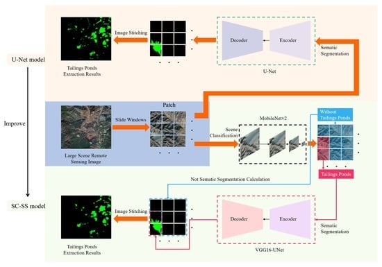
2.1. SC-SS Model

To improve the quality and efficiency of tailings pond extraction, this paper designs a fast tailings pond extraction method (SC-SS) combining scene classification and semantic segmentation, which can accurately and quickly extract tailings ponds from remote sensing images of large scenes (Figure 1). First, large scene remote sensing images are cropped into small-size remote sensing images of 512 × 512 based on the sliding window method. Then, the scene classification model MobileNetv2 network filters out the scenes containing tailings ponds from the cropped small-size remote sensing images. The semantic segmentation model VGG16-UNet extracts tailings ponds from the screened tailings pond scenes. Finally, the affine transformation parameters of small-size remote sensing images are used to realize image stitching, and the tailings ponds in large scene remote sensing images can be extracted. Semantic segmentation models perform calculations on all small-size remote sensing images segmented by the sliding window method while the SC-SS model only performs calculations on scenes with tailings ponds.

2.2. Scene Classification

Scene classification aims to automatically classify remote sensing scene images into a specific semantic label according to their contents, and realize image-level classification of remote sensing images. In the task of scene classification, the deep neural network has too many parameters (the number of parameters is usually tens of millions to hundreds of millions), and the amount of computation is huge, while the lightweight network requires less computation and parameters, and model inference is faster. To realize the fast classification of scenes with tailings ponds and scenes without tailings ponds, the MobileNetv2 is adopted as the scene classification network model, which considers the running speed and accuracy.

The MobileNet model [40] is a kind of lightweight convolutional neural network proposed by Google in 2017. It can be deployed on platforms with limited computing resources, such as embedded devices or mobile terminals. The model has both characteristics of low latency and high precision. Using the idea of depthwise separable convolutions, the MobileNet model decomposes the standard convolution into depthwise convolution and pointwise convolution. The principle is shown in Figure 2. First, the convolution kernel is divided into single channels by depthwise convolution, and each channel of the input feature map is convolved with the corresponding convolution kernel to obtain the feature map with the same number of channels as the input feature map. Then, pointwise convolution adopts a 1 × 1 convolution operation to realize a weighted fusion of feature maps in-depth, and the resulting map is obtained.

Table 1. Comparison of depthwise separable convolution and standard convolution.

Name	Params	FLOPs
Standard Convolution	$F_k\times F_k\times M\times N$	$F_k\times F_k\times M\times N\times F_H\times F_W$
Depthwise Separable Convolution	$F_k\times F_k\times M+M\times N$	$F_k\times F_k\times M\times F_H\times F_W+M\times N\times F_H\times F_W$

shows the parameters (Params) and floating-point operations (FLOPs) of depthwise separable convolution and standard convolution.

As seen from Table 1, the parameter ratio of depthwise separable convolution and the standard convolution is:

$$\frac{F_k\times F_k\times M+M\times N}{F_k\times F_k\times M\times N}=\frac{1}{N}+\frac{1}{F_k^2}$$

(1)

where $M$ represents the number of channels of the input feature map, $F_k$ represents the kernel size of the depthwise convolution, and $N$ represents the number of channels of the output feature map.

It can be concluded from Equation (1) that the depthwise separable convolution can effectively decrease the number of parameters and make the model inference faster.

Based on the MobileNet model, the MobileNetv2 model [41] adopts an inverted residual structure and a linear bottleneck structure. In contrast to the residual structure [42], the inverted residual structure first uses a 1 × 1 point convolution to expand the dimension, then uses 3 × 3 depthwise separable convolutions to collect features after the channel number is expanded, and uses a 1 × 1 convolution to reduce the dimension. At the same time, the dimensionality-reduced convolution module does not use ReLU6 nonlinear activation, but uses a linear function for calculation. The MobileNetv2 network structure consists of 17 modules (Figure 3).

2.3. Semantic Segmentation

The U-Net model is a new type of semantic segmentation structure based on the FCN model [43]. It can achieve a good segmentation result with a small number of datasets, and has become the mainstream method of image semantic segmentation. Compared with the FCN model, the U-Net model has a U-shaped symmetric structure (Figure 4). On the left is the encoder structure, which performs downsampling operations on the input image to capture context information. On the right is the decoder structure, which upsamples feature maps based on bilinear interpolation to restore image size. Between the encoder and the decoder, skip connection layers are used to realize the combination of deep semantic knowledge and shallow location knowledge. The encoder consists of four stages, each consisting of a different number of convolutional layers. The decoder is symmetric with the encoder, and it also contains four stages, each of which consists of two 3 × 3 convolutional layers, a ReLU activation function, and an upsampling layer. The skip connection layer is adopted to connect the output results of different stages of the encoder with the decoder part of the same layer, to achieve multiscale feature fusion.

To improve the extraction accuracy of tailings ponds based on the U-Net model and enhance the stability and adaptability of the model, we replace the encoder of the U-Net model with the VGG16 model [44] pretrained on ImageNet. The convolutional layers of VGG16 model are divided into 5 stages. The first two stages are composed of 2 convolution layers, and the last three stages are composed of 3 convolution layers. Compared with the original encoder of the U-Net model, the VGG16 model has deeper network layers and stronger feature extraction ability (Figure 5).

2.4. Evaluation Metrics

Model is evaluated by using a test set to describe the performance of the model accurately. The evaluation metric used by the scene classification model is accuracy, and the calculation formula is shown in Equation (2). The evaluation metrics used by the semantic segmentation model are Precision (P), Recall (R), F1, and Intersection over Union (IOU), and the calculation formulas are shown in Equations (3)–(6).

$$accuracy=\frac{h}{f}$$

(2)

where $h$ represents the amount of correctly classified remote sensing images, and $f$ is the total amount of classified remote sensing images.

$$P=\frac{TP}{TP+FP}$$

(3)

$$R=\frac{TP}{TP+FN}$$

(4)

$$F1=\frac{2\times P\times R}{P+R}$$

(5)

$$IOU=\frac{TP}{TP+FP+FN}$$

(6)

where $TP$ represents the amount of pixels that the model predicts the tailings pond as the tailings pond, $FN$ represents the amount of pixels that the model predicts the tailings pond as the background, and $FP$ represents the amount of pixels that the model predicts the background as the tailings pond. When the model predicts one remote sensing image, the statistical range of the pixel number of $TP$, $FN$, and $FP$ is one image; when the model predicts multiple remote sensing images, the statistical range of the pixel number of $TP$, $FN$, and $FP$ is multiple images.

3. Experiments and Results

3.1. Study Area and Data

3.1.1. Study Area

Luanping County is located northwest of Chengde City, Hebei Province, China, with a longitude of 116°40′~117°46′E and a latitude of 40°39′~41°12′N. It is rich in mineral resources. With the development of industry, the number of tailings ponds is increasing, which poses a huge potential safety hazard [45]. Once an accident happens in tailings ponds, it will cause casualties and release toxic pollutants [46]. It is of paramount importance for the safe operation of tailings ponds to have a dynamic monitoring system that can be used in real-time. There are more than 30 kinds of available mineral resources in Luanping County, of which the iron ore reserves reach 3 billion tons. Therefore, Luanping County is selected as the research area in this paper, as shown in Figure 6.

3.1.2. Experimental Data

In this experiment, Google Earth images with 2 m resolution and the R, G and B bands were used as data sources. Google Earth images are stitched together from multiple sensor data, so the date of large scene remote sensing images is not consistent. We use QGIS to download Google Earth images, the download link is https://mt0.google.com/vt/lyrs=s&hl=en&x={x}&y={y}&z={z}, and the download date is 19 September 2022. The datasets of tailings ponds are distributed in four areas A~D, as shown in Figure 7. The size of each area is 11,264 × 9728, among which there are more tailings ponds in area A, but fewer tailings ponds in areas B, C and D. Therefore, the tailings ponds in area A are selected to make a semantic segmentation dataset by pixel-level annotation, and the annotation tool is the QGIS software. Meanwhile, the tailings ponds and backgrounds in areas A, B, C and D are selected and the scene classification dataset is created by image-level annotations. In the annotation process, the tailings pond is marked by a manual visual interpretation method.

Considering the limitation of GPU memory, many images with a size of 512 × 512 are randomly cropped for the images and labels in four regions, and the cropping positions are randomly selected and evenly distributed. Finally, the semantic segmentation dataset has 600 samples, and the scene classification dataset has 2700 samples. These two datasets are randomly split into the training, validation, and test sets in the ratio of 8:1:1, respectively. Figure 8 and Figure 9 show examples of tailings ponds for the datasets.

3.2. Experimental Setup

The training and testing of all models in the experiment are carried out on a Dell laptop, which is configured as an Intel(R) Core (TM) i7-10870H CPU @ 2.40 GHz, 16 GB RAM, NVIDIA GeForce RTX 3060 Laptop GPU, and Windows 10 operating system. The framework used for model building is PyTorch 1.7.1 and Torchvision 0.8.2, and the code is written in Python 3.8.13. The loss function used for model training is cross entropy loss. The optimizer used is the Adam algorithm, and the learning rate decay strategy is the periodic learning rate decay (StepLR), with an initial learning rate of 0.0001, a decay factor of 0.96 and a decay step size of 1. The model’s input size is 512 × 512, the batch size is 2, the maximum number of iterations for the scene classification model is 50 epochs, and the maximum number of iterations for the semantic segmentation model is 150 epochs.

3.3. Experimental Results of the SC-SS Model

3.3.1. Tailings Pond Extraction Using MobileNetv2

The MobileNetv2 model was trained and tested utilizing the constructed tailings pond scene classification dataset. In Figure 10, the loss curves for the training set and validation set during training process are presented. The model’s accuracy on the validation set reached its highest value at the 39th epoch, and the model’s accuracy on the test set was 95.56%.

3.3.2. Tailings Pond Extraction Using VGG16-UNet

The U-Net model and VGG16-UNet model were trained and tested by using the constructed semantic segmentation dataset of tailings ponds. Figure 11 is a comparison of the loss curves of the training set. Based on the figure, the training of the two models has converged. As compared with the U-Net model, the VGG16-UNet model is faster to converge and the loss value is smaller. To verify the performance of the model, the two models were tested on the test set, and the test results are displayed in

Table 2. Comparison of the test set’s evaluation metrics for the two models.

Model	P	R	F1	IOU	Input Size	Time (s)
U-Net	94.23%	94.85%	94.54%	89.64%	512 × 512	0.07
VGG16-UNet	98.90%	98.95%	98.93%	97.88%	512 × 512	0.09

.

The VGG16-UNet model has an IOU of 97.88%, which is 8.24% higher than U-Net (Table 2). For recognition speed, the VGG16-UNet model is 0.02 s lower than that of the U-Net model, which does not affect the recognition result. Overall, the VGG16-UNet model’s accuracy has significantly increased, while the speed loss is minimal.

Figure 12 illustrates the test set prediction results for the two models, where remote sensing images input to models are shown in the first column, and ground truth images are presented in the second column. Based on Figure 12, we can conclude that the VGG16-UNet model has improved tailings pond integrity over the U-Net model since the VGG16 model has a deeper network layer and a greater ability to retain details than the original encoder of the U-Net model.

3.4. Comparison of Different Methods

Since data collection area A contains most of the tailings ponds in Luanping County, and this area simultaneously contains semantic segmentation labels and scene classification labels, it can confirm the SC-SS model’s effectiveness to identify tailings ponds from large scene images. Therefore, the remote sensing image of the dataset A area with a size of 11,264 × 9728 is chosen in this paper for testing.

The sliding window size is 512 × 512, and the step size is 512 on the remote sensing image of this large scene. Finally, 117 scenes with tailings pond and 301 scenes without tailings pond are cropped. The evaluation results of different models are presented in

Table 3. Comparison of three models’ evaluation metrics on the large scene remote sensing image.

Model	P	R	F1	IOU	Time (s)
U-Net	83.26%	93.01%	87.87%	78.36%	30.99
VGG16-UNet	91.43%	98.14%	94.67%	89.88%	36.59
SC-SS	96.26%	97.00%	96.63%	93.4%	19.92

. The scene classification results of the MobileNetv2 are listed in

Table 4. Prediction results of the MobileNetv2 model on large scene remote sensing images.

Model	Scenes with Tailings Ponds	Scenes without Tailings Ponds	Accuracy	Time (s)
MobileNetv2	131	287	86.60%	8.45

.

According to the analysis in Table 3, the SC-SS model has better evaluation metrics than the U-Net model and extracts tailings ponds from large scene remote sensing images with higher extraction accuracy and a faster extraction speed. The main reason is that when extracting tailings ponds from large scene remote sensing images, the scene without tailings ponds of the SC-SS model does not perform the final semantic segmentation calculation, which suppresses the background interference, improving the model extraction accuracy as well as speeding up the model extraction process. In addition, the VGG16 model of the semantic segmentation stage has stronger feature extraction capabilities. Compared with the VGG16-UNet model, the SC-SS model adds the stage of scene classification. Although the SC-SS has a lower recall metric than the VGG16-UNet, the remaining evaluation metrics are higher than that of the VGG16-UNet model. The main reason is that the proportion of tailings ponds in some tailings pond scenes is very small (small than 29 × 29 pixels), which leads to the scene classification model identifying the scene as a background scene, which has some influence on the recall metric. However, the SC-SS model surpasses the VGG16-UNet model in terms of comprehensive evaluation metrics F1, IOU and extraction speed, so the SC-SS model outperforms the VGG16-UNet model in performance.

Table 4 illustrates the extraction results of the large scene remote sensing images in the scene classification stage of the SC-SS model. The calculation time of the model on 418 small scene remote sensing images is only 8.45 s, which is due to the lightweight characteristics of the MobileNetv2 model, while the inference times of the U-Net model and the VGG16-UNet model are 30.99 s and 36.59 s, respectively. When extracting tailings ponds from large scene remote sensing images, the SC-SS model only uses 131 small scene remote sensing images to carry out the final semantic segmentation calculation. Therefore, the total extraction time of the model is 19.92 s, which is 35.72% shorter than the U-Net model.

Figure 13 illustrates the extraction results of tailings ponds by three models in the large scene remote sensing images. The tailings pond extracted by the SC-SS model is closest to the ground truth (Figure 13), indicating that this model can reduce background interference and improve the accuracy of tailings pond extraction.

4. Discussion

The SC-SS model has advantages in extraction accuracy and extraction speed when extracting tailings ponds from large scene images. First, the SC-SS model selects the lightweight model MobileNetv2 to complete the classification of scenes with tailings ponds and scenes without tailings ponds, and to realize the screening of potential areas of tailings ponds. Then, based on the VGG16-UNet model, only the tailings pond scene is finely segmented. In this process, the scene without tailings ponds does not participate in the final semantic segmentation calculation, so the extraction speed of the tailings ponds is faster. At the same time, it eliminates the disturbance of the complicated background scene to improve the accuracy of tailings pond extraction. More importantly, the SC-SS model performs better when tailings ponds are rare in large scene images.

The VGG16-UNet model is a further optimization of the U-Net model. By replacing the U-Net models encoder with the VGG16 model pretrained on ImageNet, the accuracy of tailings pond extraction is improved because the VGG16 model has deeper network layers and stronger feature extraction ability.

In terms of extraction accuracy, the SC-SS model can realize the pixel-level extraction of tailings ponds, while the scene classification model [41] and the object detection model [34] can only identify the approximate scope of tailings ponds. In terms of extraction speed, the SC-SS model reduces the interference and redundant calculations of complex scenes without tailings ponds by combining the scene classification model, which has higher accuracy and efficiency. However, the semantic segmentation model [37] has more redundant calculations and is disturbed by complex backgrounds, so its accuracy and efficiency are low.

By summarizing the experimental results, it is found that some objects are identified as tailings ponds, mainly because the tailings ponds are composed of tailings pond residues and wastewater. The color and texture of these components are quite similar to those of objects such as water bodies, vegetation, and clouds, leading to some misidentifications during extraction, but they are small in number.

During the monitoring process of tailings ponds, changes in the spatial scope of tailings ponds may be related to factors such as tailings dam failures, climate, mining activities and types of tailings ponds. In future research, the combination of remote sensing data with meteorological data, mining production data and tailings ponds type data can further identify and analyze the reasons for changes in the spatial scope of tailings ponds.

Due to the limited number of remote sensing images in datasets, the scope of application of this work is limited. In future research, the number of remote sensing images will be further expanded, and a larger and richer sample will be constructed by considering factors such as remote sensing image sensors, seasonal changes, and eventually, this work will be extended to other regions. Meanwhile, distinguishing the types of tailings ponds, such as active or inactive, will be the next research goal.

For the scene classification model, the transformer structure [47,48,49] can achieve overall perception and the macroscopic understanding of remote sensing images, especially for large scenes. Therefore, in future research, the transformer structure is introduced for the scene classification model, to further improve the robustness and generalization ability of tailings pond scenes and realize the accurate extraction of the potential range of tailings ponds. With the development of light and small UAVs and the research of various sensors, the type, quality and quantity of remote sensing data have been greatly increased. Therefore, multimodal data (such as, SAR, DEM, LiDAR and hyperspectral data) can be incorporated into the semantic segmentation model, and the misidentification of similar objects can be reduced by using rich spectrum, elevation, and other features.

5. Conclusions

To realize the accurate and fast extraction of tailings ponds from large scene remote sensing images, this paper proposed the tailings pond extraction model SC-SS. The model consisted of two stages: scene classification and semantic segmentation. Among them, in the scene classification stage, the MobileNetv2 was used to realize high-precision and the fast classification of scenes with tailings pond and scenes without tailings pond, which was used to eliminate the interference of complex backgrounds. The semantic segmentation stage was based on the U-Net model. To improve the extraction accuracy of tailings ponds, the pretrained VGG16 was introduced in the encoding stage to replace the original convolutional layer. In this paper, Luanping County was taken as the research area, and high-resolution Google Earth images were used as the experimental data to generate the tailings pond scene classification dataset and tailings pond semantic segmentation dataset for model training and testing. The scene classification dataset of tailings ponds contained 2700 samples, and the semantic segmentation dataset of tailings ponds contained 600 samples. Finally, based on the self-built tailings pond datasets, the training and testing of the models were completed. According to the experimental results, the extraction accuracy of IOU for the SC-SS model was 93.48%. The extraction accuracy IOU was increased by 15.12% when compared to the U-Net model, and the extraction time was shortened by 35.72%. This study can realize the large-scale remote sensing dynamic monitoring of tailings ponds and provide a reference for ecological environment restoration.

References

- Wang, C.; Harbottle, D.; Liu, Q.; Xu, Z. Current state of fine mineral tailings treatment: A critical review on theory and practice. Miner. Eng. 2014, 58, 113–131. [Google Scholar] [CrossRef]
- Komljenovic, D.; Stojanovic, L.; Malbasic, V.; Lukic, A. A resilience-based approach in managing the closure and abandonment of large mine tailing ponds. Int. J. Min. Sci. Technol. 2020, 30, 737–746. [Google Scholar] [CrossRef]
- Small, C.C.; Cho, S.; Hashisho, Z.; Ulrich, A.C. Emissions from oil sands tailings ponds: Review of tailings pond parameters and emission estimates. J. Pet. Sci. Eng. 2015, 127, 490–501. [Google Scholar] [CrossRef]
- Rotta, L.H.S.; Alcântara, E.; Park, E.; Negri, R.G.; Lin, Y.N.; Bernardo, N.; Mendes, T.S.G.; Souza Filho, C.R. The 2019 Brumadinho tailings dam collapse: Possible cause and impacts of the worst human and environmental disaster in Brazil. Int. J. Appl. Earth Obs. Geoinf. 2020, 90, 102119. [Google Scholar] [CrossRef]
- Wang, Y.; Yang, Y.; Li, Q.; Zhang, Y.; Chen, X. Early Warning of Heavy Metal Pollution after Tailing Pond Failure Accident. J. Earth Sci. 2022, 33, 1047–1055. [Google Scholar] [CrossRef]
- Yan, D.; Zhang, H.; Li, G.; Li, X.; Lei, H.; Lu, K.; Zhang, L.; Zhu, F. Improved Method to Detect the Tailings Ponds from Multispectral Remote Sensing Images Based on Faster R-CNN and Transfer Learning. Remote Sens. 2022, 14, 103. [Google Scholar] [CrossRef]
- Oparin, V.N.; Potapov, V.P.; Giniyatullina, O.L. Integrated assessment of the environmental condition of the high-loaded industrial areas by the remote sensing data. J. Min. Sci. 2014, 50, 1079–1087. [Google Scholar] [CrossRef]
- Song, W.; Song, W.; Gu, H.; Li, F. Progress in the remote sensing monitoring of the ecological environment in mining areas. Int. J. Environ. Res. Public Health 2020, 17, 1846. [Google Scholar] [CrossRef] [PubMed] [Green Version]
- Lumbroso, D.; Collell, M.R.; Petkovsek, G.; Davison, M.; Liu, Y.; Goff, C.; Wetton, M. DAMSAT: An eye in the sky for monitoring tailings dams. Mine Water Environ. 2021, 40, 113–127. [Google Scholar] [CrossRef]
- Li, H.; Xiao, S.; Wang, X.; Ke, J. High-resolution remote sensing image rare earth mining identification method based on Mask R-CNN. J. China Univ. Min. Technol. 2020, 49, 1215–1222. [Google Scholar] [CrossRef]
- Chen, T.; Zheng, X.; Niu, R.; Plaza, A. Open-Pit Mine Area Mapping with Gaofen-2 Satellite Images Using U-Net+. IEEE J. Sel. Top. Appl. Earth Obs. Remote Sens. 2022, 15, 3589–3599. [Google Scholar] [CrossRef]
- Rivera, M.J.; Luís, A.T.; Grande, J.A.; Sarmiento, A.M.; Dávila, J.M.; Fortes, J.C.; Córdoba, F.; Diaz-Curiel, J.; Santisteban, M. Physico-chemical influence of surface water contaminated by acid mine drainage on the populations of diatoms in dams (Iberian Pyrite Belt, SW Spain). Int. J. Environ. Res. Public Health 2019, 16, 4516. [Google Scholar] [CrossRef] [PubMed] [Green Version]
- Rossini-Oliva, S.; Mingorance, M.; Peña, A. Effect of two different composts on soil quality and on the growth of various plant species in a polymetallic acidic mine soil. Chemosphere 2017, 168, 183–190. [Google Scholar] [CrossRef] [PubMed]
- Tang, L.; Liu, X.; Wang, X.; Liu, S.; Deng, H. Statistical analysis of tailings ponds in China. J. Geochem. Explor. 2020, 216, 106579. [Google Scholar] [CrossRef]
- Ke, R.; Bugeau, A.; Papadakis, N.; Kirkland, M.; Schuetz, P.; Schönlieb, C.-B. Multi-Task Deep Learning for Image Segmentation Using Recursive Approximation Tasks. IEEE Trans. Image Process. 2021, 30, 3555–3567. [Google Scholar] [CrossRef] [PubMed]
- Jiang, Y.; Gong, X.; Liu, D.; Cheng, Y.; Fang, C.; Shen, X.; Yang, J.; Zhou, P.; Wang, Z. EnlightenGAN: Deep Light Enhancement without Paired Supervision. IEEE Trans. Image Process. 2021, 30, 2340–2349. [Google Scholar] [CrossRef]
- Fan, M.; Lai, S.; Huang, J.; Wei, X.; Chai, Z.; Luo, J.; Wei, X. Rethinking BiSeNet for real-time semantic segmentation. In Proceedings of the IEEE/CVF Conference on Computer Vision and Pattern Recognition (CVPR), Nashville, TN, USA, 20–25 June 2021; pp. 9716–9725. [Google Scholar]
- Yuan, Y.; Fang, J.; Lu, X.; Feng, Y. Remote Sensing Image Scene Classification Using Rearranged Local Features. IEEE Trans. Geosci. Remote Sens. 2018, 57, 1779–1792. [Google Scholar] [CrossRef]
- Zhang, X.; Yue, Y.; Gao, W.; Yun, S.; Su, Q.; Yin, H.; Zhang, Y. DifUnet++: A Satellite Images Change Detection Network Based on Unet++ and Differential Pyramid. IEEE Geosci. Remote Sens. Lett. 2021, 19, 1–5. [Google Scholar] [CrossRef]
- Zakria, Z.; Deng, J.; Kumar, R.; Khokhar, M.S.; Cai, J.; Kumar, J. Multiscale and Direction Target Detecting in Remote Sensing Images via Modified YOLO-v4. IEEE J. Sel. Top. Appl. Earth Obs. Remote Sens. 2022, 15, 1039–1048. [Google Scholar] [CrossRef]
- Xu, G.; Wu, X.; Zhang, X.; He, X. LeviT-UNet: Make faster encoders with transformer for medical image segmentation. arXiv 2021, arXiv:2107.08623. [Google Scholar] [CrossRef]
- Huang, X.; Deng, Z.; Li, D.; Yuan, X. MISSformer: An effective medical image segmentation transformer. arXiv 2021, arXiv:2109.07162. [Google Scholar] [CrossRef]
- Huang, H.; Lin, L.; Tong, R.; Hu, H.; Zhang, Q.; Iwamoto, Y.; Han, X.; Chen, Y.-W.; Wu, J. UNet 3+: A full-scale connected unet for medical image segmentation. In Proceedings of the 2020 IEEE International Conference on Acoustics, Speech and Signal Processing (ICASSP 2020), Barcelona, Spain, 4–8 May 2020; pp. 1055–1059. [Google Scholar]
- Gorelick, N.; Hancher, M.; Dixon, M.; Ilyushchenko, S.; Thau, D.; Moore, R. Google Earth Engine: Planetary-scale geospatial analysis for everyone. Remote Sens. Environ. 2017, 202, 18–27. [Google Scholar] [CrossRef]
- Yuan, Q.; Shen, H.; Li, T.; Li, Z.; Li, S.; Jiang, Y.; Xu, H.; Tan, W.; Yang, Q.; Wang, J.; et al. Deep learning in environmental remote sensing: Achievements and challenges. Remote Sens. Environ. 2020, 241, 111716. [Google Scholar] [CrossRef]
- Shi, W.; Zhang, M.; Zhang, R.; Chen, S.; Zhan, Z. Change detection based on artificial intelligence: State-of-the-art and challenges. Remote Sens. 2020, 12, 1688. [Google Scholar] [CrossRef]
- Zhu, X.X.; Montazeri, S.; Ali, M.; Hua, Y.; Wang, Y.; Mou, L.; Shi, Y.; Xu, F.; Bamler, R. Deep learning meets SAR: Concepts, models, pitfalls, and perspectives. IEEE Geosci. Remote Sens. Mag. 2021, 9, 143–172. [Google Scholar] [CrossRef]
- Zhang, J.; Zhang, M.; Pan, B.; Shi, Z. Semisupervised center loss for remote sensing image scene classification. IEEE J. Sel. Top. Appl. Earth Obs. Remote Sens. 2020, 13, 1362–1373. [Google Scholar] [CrossRef]
- Li, K.; Wan, G.; Cheng, G.; Meng, L.; Han, J. Object detection in optical remote sensing images: A survey and a new benchmark. ISPRS J. Photogramm. Remote Sens. 2020, 159, 296–307. [Google Scholar] [CrossRef]
- Yuan, X.; Shi, J.; Gu, L. A review of deep learning methods for semantic segmentation of remote sensing imagery. Expert Syst. Appl. 2021, 169, 114417. [Google Scholar] [CrossRef]
- Li, Q.; Chen, J.; Li, Q.; Li, B.; Lu, K.; Zan, L.; Chen, Z. Detection of tailings pond in Beijing-Tianjin-Hebei region based on SSD model. Remote Sens. Technol. Appl. 2021, 36, 293–303. [Google Scholar]
- Liu, B.; Xing, X.; Wu, H.; Hu, S.; Zan, J. Remote sensing identification of tailings pond based on deep learning model. Sci. Surv. Mapp. 2021, 46, 129–139. [Google Scholar]
- Zhang, K.; Chang, Y.; Pan, J.; Lu, K.; Zan, L.; Chen, Z. Tailing pond extraction of Tangshan City based on Multi-Task-Branch Network. J. Henan Polytech. Univ. Nat. Sci. 2022, 41, 65–71, 94. [Google Scholar]
- Liu, W.; Anguelov, D.; Erhan, D.; Szegedy, C.; Reed, S.; Fu, C.-Y.; Berg, A.C. SSD: Single shot multibox detector. In Computer Vision–ECCV 2016, Proceedings of the European Conference on Computer Vision 2016 (ECCV 2016), Amsterdam, The Netherlands, 8–16 October 2016; Leibe, B., Matas, J., Sebe, N., Welling, M., Eds.; Springer: Cham, Switzerland, 2016; Volume 9905, pp. 21–37. [Google Scholar]
- Ren, S.; He, K.; Girshick, R.; Sun, J. Faster R-CNN: Towards real-time object detection with region proposal networks. IEEE Trans. Pattern Anal. Mach. Intell. 2017, 39, 1137–1149. [Google Scholar] [CrossRef] [PubMed] [Green Version]
- Kai, Y.; Ting, S.; Zhengchao, C.; Hongxuan, Y. Automatic extraction of tailing pond based on SSD of deep learning. J. Univ. Chin. Acad. Sci. 2020, 37, 360. [Google Scholar] [CrossRef]
- Ronneberger, O.; Fischer, P.; Brox, T. U-Net: Convolutional networks for biomedical image segmentation. In Medical Image Computing and Computer-Assisted Intervention–MICCAI 2015, Proceedings of the International Conference on Medical Image Computing and Computer-Assisted Intervention (MICCAI 2015), Munich, Germany, 5–9 October 2015; Navab, N., Hornegger, J., Wells, W., Frangi, A., Eds.; Springer: Cham, Switzerland, 2015; Volume 9351, pp. 234–241. [Google Scholar]
- Zhang, C.; Xing, J.; Li, J.; Sang, X. Recognition of the spatial scopes of tailing ponds based on U-Net and GF-6 images. Remote Sens. Land Resour. 2021, 33, 252–257. [Google Scholar] [CrossRef]
- Lyu, J.; Hu, Y.; Ren, S.; Yao, Y.; Ding, D.; Guan, Q.; Tao, L. Extracting the Tailings Ponds from High Spatial Resolution Remote Sensing Images by Integrating a Deep Learning-Based Model. Remote Sens. 2021, 13, 743. [Google Scholar] [CrossRef]
- Howard, A.G.; Zhu, M.; Chen, B.; Kalenichenko, D.; Wang, W.; Weyand, T.; Andreetto, M.; Adam, H. MobileNets: Efficient convolutional neural networks for mobile vision applications. arXiv 2017, arXiv:1704.04861. [Google Scholar]
- Sandler, M.; Howard, A.; Zhu, M.; Zhmoginov, A.; Chen, L.-C. Mobilenetv2: Inverted residuals and linear bottlenecks. In Proceedings of the IEEE Conference on Computer Vision and Pattern Recognition 2018 (CVPR 2018), Salt Lake City, UT, USA, 18–23 June 2018; pp. 4510–4520. [Google Scholar]
- He, K.; Zhang, X.; Ren, S.; Sun, J. Deep residual learning for image recognition. In Proceedings of the IEEE Conference on Computer Vision and Pattern Recognition 2016 (CVPR 2016), Las Vegas, NV, USA, 27–30 June 2016; pp. 770–778. [Google Scholar]
- Liu, A.; Yang, Y.; Sun, Q.; Xu, Q. A deep fully convolution neural network for semantic segmentation based on adaptive feature fusion. In Proceedings of the 5th International Conference on Information Science and Control Engineering (ICISCE 2018), Zhengzhou, China, 20–22 July 2018; pp. 16–20. [Google Scholar] [CrossRef]
- Simonyan, K.; Zisserman, A. Very deep convolutional networks for large-scale image recognition. arXiv 2014, arXiv:1409.1556. [Google Scholar]
- Lin, S.-Q.; Wang, G.-J.; Liu, W.-L.; Zhao, B.; Shen, Y.-M.; Wang, M.-L.; Li, X.-S. Regional Distribution and Causes of Global Mine Tailings Dam Failures. Metals 2022, 12, 905. [Google Scholar] [CrossRef]
- Cheng, D.; Cui, Y.; Li, Z.; Iqbal, J. Watch Out for the Tailings Pond, a Sharp Edge Hanging over Our Heads: Lessons Learned and Perceptions from the Brumadinho Tailings Dam Failure Disaster. Remote Sens. 2021, 13, 1775. [Google Scholar] [CrossRef]
- Vaswani, A.; Shazeer, N.; Parmar, N.; Uszkoreit, J.; Jones, L.; Gomez, A.N.; Kaiser, Ł.; Polosukhin, I. Attention is all you need. In Proceedings of the Advances in Neural Information Processing Systems 2017 (NIPS 2017), Long Beach, CA, USA, 4–9 December 2017; Volume 30. [Google Scholar]
- Dosovitskiy, A.; Beyer, L.; Kolesnikov, A.; Weissenborn, D.; Zhai, X.; Unterthiner, T.; Dehghani, M.; Minderer, M.; Heigold, G.; Gelly, S. An image is worth 16x16 words: Transformers for image recognition at scale. arXiv 2020, arXiv:2010.11929. [Google Scholar]
- Roy, S.K.; Deria, A.; Hong, D.; Rasti, B.; Plaza, A.; Chanussot, J. Multimodal fusion transformer for remote sensing image classification. arXiv 2022, arXiv:2203.16952. [Google Scholar]