Article

Aerosol Retrieval Study from a Particulate Observing Scanning Polarimeter Onboard Gao-Fen 5B without Prior Surface Knowledge, Based on the Optimal Estimation Method

1
Key Laboratory of General Optical Calibration and Characterization Technology, Hefei Institutes of Physical Science, Chinese Academy of Sciences, Hefei 230031, China
2
Science Island Branch of Graduate School, University of Science and Technology of China, Hefei 230026, China
3
Chief Studio of Agricultural Industry in Hefei, Hefei 230031, China
*
Author to whom correspondence should be addressed.
Remote Sens. 2023, 15(2), 385; https://doi.org/10.3390/rs15020385
Submission received: 5 December 2022 / Revised: 3 January 2023 / Accepted: 6 January 2023 / Published: 8 January 2023
(This article belongs to the Special Issue Aerosol and Atmospheric Correction)

Abstract

:
To meet the demand for the aerosol detection of single-angle and multi-band polarization instrument containing short-wave infrared bands, an inversion algorithm that makes full use of multi-band intensity and polarization information is proposed based on optimal estimation theory. This method uses the polarization information in the short-wave infrared band to perform surface and atmosphere decoupling without a prior information on the surface. This obtains the initial value of the aerosol, and then it uses the scalar information to obtain the final result. Moreover, the multi-band information of the instrument is used for decoupling the surface and atmospheric information, which avoids the inversion error caused by the untimely update of the surface reflectance database and the error of spatio-temporal matching. The measured data of the Particulate Observing Scanning Polarimeter (POSP) are used to test the proposed algorithm. Firstly, to verify the effectiveness of the algorithm under different surface conditions, four regions with large geographical differences (Beijing, Hefei, Baotou, and Taiwan) are selected for aerosol optical depth (AOD) inversion, and they are compared with the aerosol robotic network (AERONET) products of the nearby stations. The validation against the AERONET products produces high correlation coefficients of 0.982, 0.986, 0.718, and 0.989, respectively, which verifies the effectiveness of the algorithm in different regions. Further, we analyzed the effectiveness of the proposed algorithm under different pollution conditions. Regions with AOD >0.7 and AOD < 0.7 are screened by using the AOD products of the Moderate-Resolution Imaging Spectroradiomete (MODIS), and the AOD of the corresponding region is inverted using POSP data. It was found to be spatially consistent with the MODIS products. The correlation coefficient and root mean square error (RMSE) in the AOD high region were 0.802 and 0.217, respectively, and 0.944 and 0.022 in the AOD low region, respectively, which verified the effectiveness of the proposed algorithm under different pollution conditions.

1. Introduction

Atmospheric aerosol, solid or liquid particles suspended in the atmosphere, including those from natural and anthropogenic sources, are an important component of the Earth’s atmosphere and they play an important role in the climate system and atmospheric environment system. In the climate system, aerosol not only affects the radiative energy balance by interacting with solar and terrestrial radiation [1,2,3], but they also change the characteristics and lifetimes of clouds [4,5,6,7,8]. In terms of the environment, aerosols are considered to be the main cause of air pollution, and they have a significant negative impact on human health [9,10,11,12,13,14,15]. Therefore, it is of great significance to carry out the remote sensing retrieval of aerosol and particulate matter concentration.
According to different remote sensing platforms, aerosol remote sensing can be divided into ground-based, airborne, and satellite remote sensing. Satellite remote sensing has the advantages of timeliness, periodicity, and large scale, and it is an effective method for detecting the optical properties and spatial distributions of aerosols [16,17,18,19,20]. The inversion of aerosol properties using satellite data has been carried out for more than 40 years. According to the difference of remote sensing data and the method of surface-atmosphere decoupling, the following methods are mainly used: dark target method using the statistical relationship between the apparent reflectance of short-wave infrared channels and the surface reflectance of red and blue channels [21,22,23]; deep blue algorithm for bright surface area [24,25]; in the Multi-angle Imaging SpectroRadiometer (MISR) operational aerosol retrieval algorithm, a mathematical method, empirical orthogonal functions, is used to obtain the surface contribution, which gives a general solution for the surface reflectance estimation in multi-angle aerosol remote sensing [26,27,28]; Inversion of aerosol optical thickness using polarization information [29,30,31,32,33,34].
Although for the aerosol inversion, lookup table (LUT)-based methods are widely applied, the method turned out to be incapable of fully exploiting the information implicit in the satellite measurements [35]. So, the optimal estimation theory is introduced into atmospheric research. The optimal estimation method was applied early to ground-based observations [36]. After that Dubovik et al. developed the generalized retrieval of an aerosol and surface properties algorithm which can be applied to a multi-angle observation satellite such as Polarization and Directionality of the Earth’s Reflectance (POLDER) [37]. There are some inversion framework based on optimal estimation theory that have been established [38,39,40,41]. Nevertheless, further studies based on optimal estimation theory need to be developed to apply to different satellite measurements such as single-angle multi-band polarization measurements, including short-wave infrared band.
The Particulate Observing Scanning Polarimeter (POSP) on board the Gaofen-5B satellite obtains atmospheric information in three dimensions: spectrum, observation angle and polarization through time synchronization and spatial coverage, and it obtains atmospheric parameters over the imaging area. The unique advantage of POSP is that it has nine detection channels from 380 to 2250 nm, all of which have polarization detection capabilities. Although its observation mode is single-angle observation, its advantages of multiple detection bands, wide band range and polarization detection capability will help with the inversion of aerosol optical depth (AOD).
According to the characteristics of POSP instruments, the intensity polarization joint inversion algorithm is proposed on the basis of optimal inversion theory, which makes full use of multi-band information. Firstly, the polarization reflectance in the 2250 nm band is used as the initial value of the surface polarization reflectance, and the optimal aerosol column concentration is obtained via the optimization iterative method. Then, according to the preliminary obtained AOD, the scalar signal is subjected to atmospheric correction to obtain the initial value of surface reflectance. Scalar information is used for the optimization iteration to obtain the final AOD.
This paper is divided into four parts: firstly, the characteristics of POSP data and the theory of optimization inversion framework are introduced. Secondly, the implementation details of the intensity polarization joint inversion algorithm are introduced in detail. Then, the effectiveness of the algorithm is tested in different regions and under different pollution conditions. Finally, the relevant conclusions are given.

2. Data and Optimization Estimate Framework

2.1. POSP Data Introduction

POSP is a high-precision polarization scanner developed by Anhui Institute of Optics and Fine Mechanics, Hefei Institute of Physical Sciences, Chinese Academy of Sciences, which is an onboard satellite for earth observation and can obtain multispectral and polarized radiation information on the surface and in the atmosphere. POSP adopts an on-board calibration to ensure the measurement accuracy and accuracy of the POSP operation in orbit [42]. POSP provides the first three components (I, Q, and U) of the Stokes vector corresponding to the band, and the basic parameters are shown in Table 1.
Since the 380 nm band is greatly influenced by atmospheric molecules, the 1380 nm band is mainly used for cirrus detection. So, seven bands except for 380 nm and 1380 nm are used for AOD inversion in this paper.

2.2. Optimization Estimate Framework

The optimal inversion framework in this paper is based on the previous information analysis of aerosol [43] plus the solution of the cost function. Let x be a state vector composed of n parameters (such as aerosol volume, refractive index, particle size distribution, etc.). The state vector will be retrieved from the observation vector y containing m measured elements, such as spectral scalar and polarization reflectivity. The relationship between y and x is shown in Formula (1):
y = F x +
where the forward model F describes the forward model of the physical relationship between y and x. ∈ represents the combined error of observation uncertainty and forward model uncertainty.
For satellite remote sensing, the forward model F is a nonlinear function, and the optimized solution of Equation (1) needs to go through multiple Gaussian hypothesis processes. According to the maximum likelihood method, the state vector of the t’th iteration corresponds to the solution that minimizes the quadratic cost function as follows:
J x t = 1 2 [ y F x t ] T S ϵ 1 y F x t + 1 2 r a ( x t x a ) T S a 1 x t x a
In Formula (2), x t represents the state vector at the t iteration, the two terms on the right side represent the constraints on the inversion results from observation and a prior estimation, respectively. The observation error covariance S ϵ represents the uncertainty of the model and measurements. The prior error covariance S a represents the uncertainty of the prior estimate x a . r a = n / 2 , where n is the number of parameters to be inverted [44].
The process of finding the minimum value of the cost function needs to go through multiple iterations, using the LM (Levenberg-Marquardt) iterative method [45]. The state vector at the (t+1)-th iteration can be expressed as:
x t + 1 = x t [ r a + γ S a 1 + K t T S ϵ 1 K t ] 1 K t T S ϵ 1 F x t y + S a 1 x t x a
In Formula (3), γ is the LM parameter, which is initially set to 10, and is adjusted according to Rodgers’ update strategy after each iteration of x. K is called the weighting function matrix or Jacobian matrix, and it consists of the partial derivative of each forward model element with respect to each state vector element, i.e., K i , j = F i / x j , i = 1 , m ; j = 1 , n (Ki,j denotes the element in the i-th row and j-th column of matrix K, Fi is the i-th simulated measurement, and xj is the j-th element in the state vector x).

3. Optimal Estimation Inversion Algorithm

3.1. A Priori Information on Aerosols and Surface

In the framework of optimal inversion, a priori estimation is an important factor affecting the inversion results. Reasonable priori estimation can reduce the number of inversion iterations, improve the time efficiency of the algorithm and avoid unreasonable convergence results. A priori estimation mainly comes from the a priori knowledge of state vectors and non-state vectors, such as historical meteorological data, ground measured data, etc. The influence of prior estimation on inversion is manifested in two aspects: first, the a priori estimation of the state parameter is input into the inversion program as the initial value for iteration, and the prior term that constitutes the cost function constrains the final inversion result. Secondly, the reasonable values of non-state parameters can reduce the model error and improve the accuracy of the inversion results.

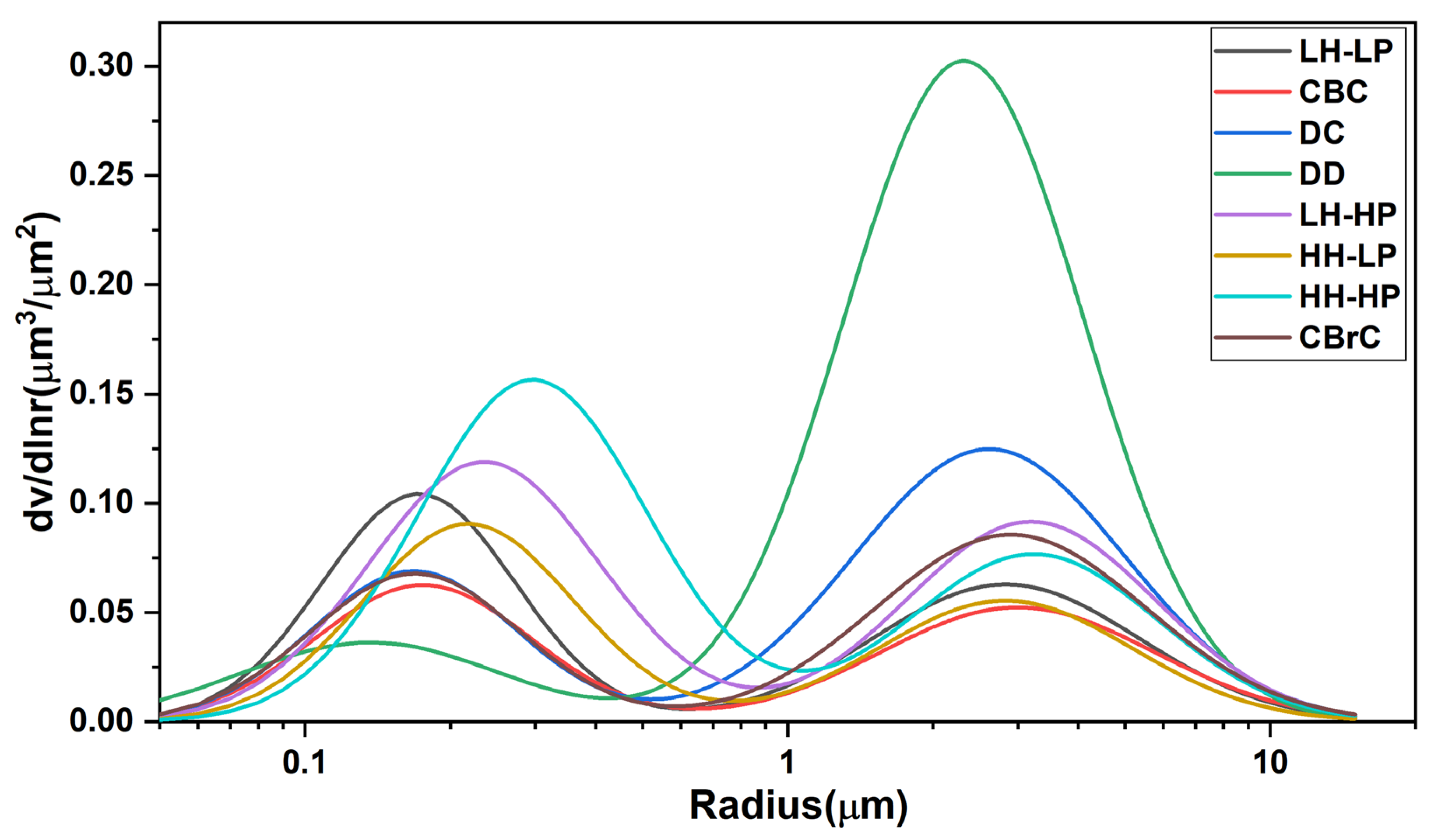
3.1.1. Aerosol Model

In many studies, the bimodal lognormal distribution function is commonly used to characterize the aerosol particle size distribution, as follows:
n r = i = 1 2 C i r σ i 2 π e x p l n r l n r m , i 2 2 σ i 2
In Formula (4), C denotes the volume concentration, σ is the standard deviation, and r m is the mean radius. The bimodal log normal distribution requires six parameters to represent.
Under the assumption of a bimodal log-normal distribution, five pairs of parameters can be used to describe the aerosol model: the particle column concentration v 0 f and v 0 c , the effective radius r e f f f and r e f f c , the effective variance v e f f f and v e f f c , the real part of the refractive index m r f and m r c , and the imaginary part of the refractive index m i f and m i c . The superscripts f and c represent fine mode particles and coarse mode particles, respectively. A priori information about the aerosol models can use the results of previous studies [46], and the aerosol particle size distribution is shown in Figure 1.
The legends in Figure 1 represent different types of aerosol models. LH-LP: Low Humidity-Low Pollution Aerosol, CBC: Carbonaceous-Black Carbon Aerosol, DC: Dust Urban Aerosol, DD: Sand Dust-Desert Aerosol, LH-HP: Low Humidity-High Pollution type aerosol, HH-LP: High Humidity-Low Pollution type aerosol, HH-Hp: High Humidity-High Pollution type aerosol, CBrC: Carbonaceous-Brown Carbon type aerosol.

3.1.2. Processing of A Priori Information about Surface

At present, the methods for obtaining a priori surface information mainly include the surface model method [29], the prior surface reflectivity database [24], etc. In this paper, according to the polarization reflectancenot being sensitive to band changes [47,48], the polarization reflectance of the shortwave infrared band is used as the initial value of the surface polarization reflections of other bands, and then the aerosol parameters to be retrieved are obtained according to an iterative strategy. According to the aerosol parameters obtained via polarization inversion, the atmospheric transmittance, hemispheric albedo and atmospheric path radiation are obtained using Unified Linearized Vector Radiative Transfer Model (UNL-VRTM) [47], and then the empirical value of the surface reflectance is obtained using Formula (5):
ρ s = ρ ρ 0 ρ ρ 0 S + T
In Formula (5), ρ , ρ 0 , and ρ s are the normalized reflectances of the atmospheric top, atmospheric path radiation, and surface, respectively. S and T are the atmospheric hemisphere albedo and the total atmospheric transmittance, respectively.

3.2. Intensity Polarization Joint Optimization Inversion Algorithm

3.2.1. Satellite Observation Model

The radiation signals obtained by satellites can be characterized by the apparent reflectance. There are multiple interaction processes between the surface and the atmosphere, which are complicated by different surface reflectances and different atmospheric conditions. Therefore, the apparent reflectance model is as follows [49]:
R TOA μ s , μ v , φ = R Atm μ s , μ v , φ + T s T v ρ μ s , μ v , φ 1 s ρ μ s , μ v , φ R TOA μ s , μ v , φ = π I μ s , μ v , φ μ s E 0
In Formula (6), R TOA and R Atm are the top-of-atmosphere (TOA) reflectance and the atmospheric path radiation, T s and T v are atmospheric downward and upward transmittances, respectively, ρ is the surface albedo and s is the atmospheric hemispheric albedo. μ s ,   μ v , and φ are the cosine of the solar zenith angle, the cosine of the observed zenith angle, and the relative azimuth angle. E 0 is the solar constant (the solar spectral irradiance outside the atmosphere). The surface albedo can be obtained if the apparent reflectance, atmospheric path radiation, atmospheric transmittance, and atmospheric hemispheric albedo are known.
The polarization signal obtained by the satellite is characterized by the TOA polarized reflectance. The polarization contribution caused by the multiple interactions between the surface and the atmosphere is very small. After the attenuation of the atmosphere, the contribution to the observation at the top of the atmosphere can be ignored. Therefore, the TOA polarized reflectance modeling only needs to consider the upward polarization scattering of the atmosphere and the single reflection of the surface [50], and the TOA polarized reflectance can be written as follows:
R P TOA μ s , μ v , φ = R P Atm μ s , μ v , φ + T s ρ P μ s , μ v , φ T v R P TOA μ s , μ v , φ = π I p μ s , μ v , φ μ s E 0
In Formula (7), R P TOA is the TOA polarized reflectance, R P Atm is the polarized reflectance of the atmosphere (which can be calculated by setting the surface polarized reflectance to zero), and ρ P is the surface polarized reflectance. I p = Q 2 + U 2 is the polarized radiance at the top of the atmosphere.
In summary, when using the intensity information and polarization information for the optimization solution, due to different observation models and different assumptions of the surface, the state vector x and observation vector y are shown in Table 2:
In Table 2, the superscript T represents the transpose of the vector, and λ 1 λ 7 are the corresponding center wavelengths of POSP: 410 nm, 443 nm, 490 nm, 670 nm, 865 nm, 1610 nm and 2250 nm, respectively. V f and V c are the aerosol fine-mode and coarse-mode column concentrations, respectively, and ρ represents the surface reflectance. Since it is assumed that the surface polarized reflectance is independent of the wavelength, and the TOA polarized reflectance in the 2250 nm band is used as the initial value of the surface polarized reflectance, in the polarization inversion, the state vector x has only three parameters, and the observation vector has 6 parameters. In the intensity inversion, the state vector has nine parameters and the observation vector has seven parameters.

3.2.2. Cost Function Solution Method

The optimal estimation theory provides the cost function J(x) for finding the optimal inversion result, and gives the specific form. J(x) is a nonlinear function, and Newton’s iterative method is a common method for solving nonlinear functions. In this paper, the LM algorithm is used to solve the minimum value of J(x), and in the LM program module, the forward radiated transmission simulation module and the calculation module of the cost function are combined to establish the program framework for optimal iterative inversion. Under the framework of the program, the optimal estimation of the state vector is found after several iterations. The convergence condition is as follows:
Δ = x t + 1 x t 2 x t 2 ε
In Formula (8), where || ||2 is the L2 norm, ε is the convergence threshold for judging the end of the iteration, which is an empirical value, and is taken as 0.1% in this paper.
In the actual operation process, when the number of iterations exceeds the set maximum number of iterations of six, or when the element value in x exceeds the boundary range, the iteration stops and an invalid value is output.

3.2.3. Algorithm Implementation

The LM program module, UNL-VRTM, and the cost function calculation module are combined to make full use of the multi-band polarization information of POSP to carry out the optimal inversion of AOD. The detailed flow chart is shown in Figure 2. After reading the POSP data, the proposed algorithm can be divided into the following two stages.
In the first stage, the optimal inversion is performed using the polarization information to obtain the aerosol column concentration. There are three main steps at this stage: (1) Obtain the initial value of the surface polarization reflectivity of other bands through the apparent polarization reflectivity of 2250 nm; (2) Use the radiation transfer software UNL-VRTM to calculate the Jacobian matrix of the state vector; (3) Obtain a new state vector according to the update strategy of Formula (3), and then after several iterations, when the iterative convergence threshold is met, the aerosol column concentration parameter is output.
In the second stage, the final aerosol column concentration parameters are obtained by optimizing the inversion using the intensity information. First, input the aerosol column concentration parameters obtained in the previous stage into UNL-VRTM and run it, and then perform simple atmospheric correction according to Equation (5) to obtain the initial values of surface reflectance in different bands. Then, according to (2)–(3) of the first stage, the column concentration parameters of the aerosol are finally obtained.
The aerosol volume column concentration parameters are obtained via inversion according to the above process, and the spectral AOD can be further calculated by combining with the aerosol model parameters, but this calculation process does not need to be carried out separately. In the iterative process, when using the UNL-VRTM software for forward simulation, AOD can be obtained at the same time, and the calculation result can be output when the last step satisfies the iterative convergence condition.

4. Result and Discussion

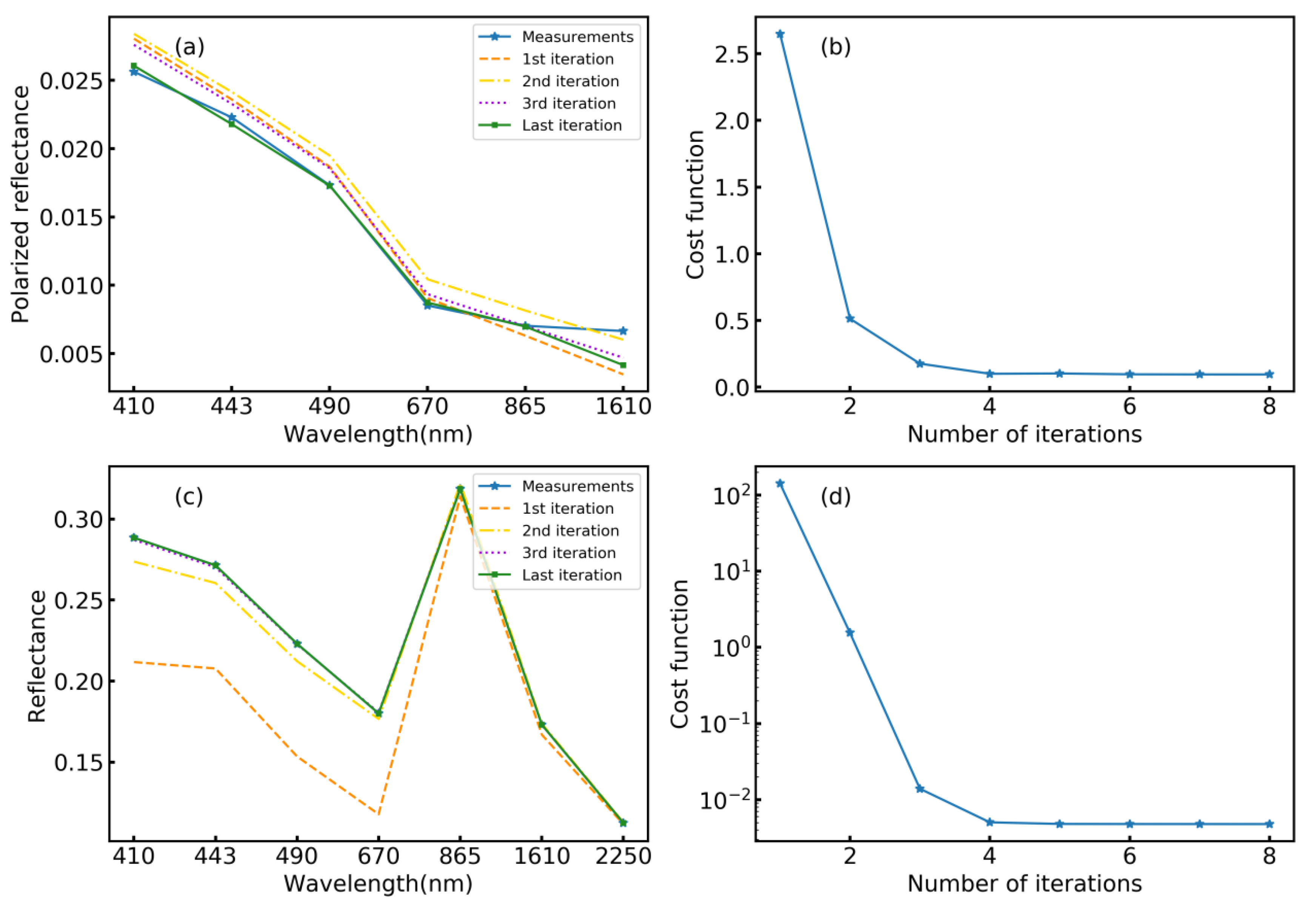
4.1. Algorithm Iteration Process

According to the prior information acquisition and retrieval strategy described above, the POSP data from November 2021 to July 2022 are selected for the retrieval of AOD. An inversion case of 8 June 2022, over the Beijing site is selected to illustrate the iteration and convergence processes of the algorithm, as shown in Figure 3.
Figure 3a,c shows the fitting between the simulated values of the model and the measured values of POSP with the increase in the number of iterations in the process of inversion using polarization information and intensity information, respectively. After the last iteration, the simulated values using polarization information agree well with the observed values in the first five bands, and there is only a slight gap in the 1610 nm band. The simulated values using intensity information are in good agreement with the observed values in all bands, indicating that in single-angle observation, the intensity contains more information about the atmosphere than the polarization measurement. In Figure 3b,d of the cost function varies with the number of iterations in the process of polarization inversion and intensity inversion, respectively. It is also reflected that the intensity contains more information than polarization from (b) and (d). When convergence, the cost function value of intensity information inversion is less than that of polarization information inversion. After five iterations, the cost function almost does not change with the increase in the number of iterations, so that in order to save the time of the algorithm, the maximum number of iterations can be set to 6.

4.2. Evaluation Index of the Inversion Result

In the evaluation of the inversion results, quantitative indexes such as correlation coefficient (R), root mean square error (RMSE), expected error (EE), and the percentage of except error (Scope) are used. Taking AOD as an example, the specific definitions of each index are as follows:
R = cov τ retrieval , τ true std τ retrieval × std τ true
RMSE = 1 N i = 1 N τ retrieval τ true 2
Δ = EE = ± 0.15 τ true ± 0.05
Scope = N valid / N × 100 %
In Formulas (9)–(12), τ retrieval is the AOD result of inversion using POSP data, and τ true is the data for verification. Cov() and std() represent the covariance and standard deviation calculations, respectively. Scope is the proportion of the amount of data within the range of τ true + Δ for the inversion AOD to the total data. N and N valid are the amount of data and the total amount of data that fall into the error range, respectively.

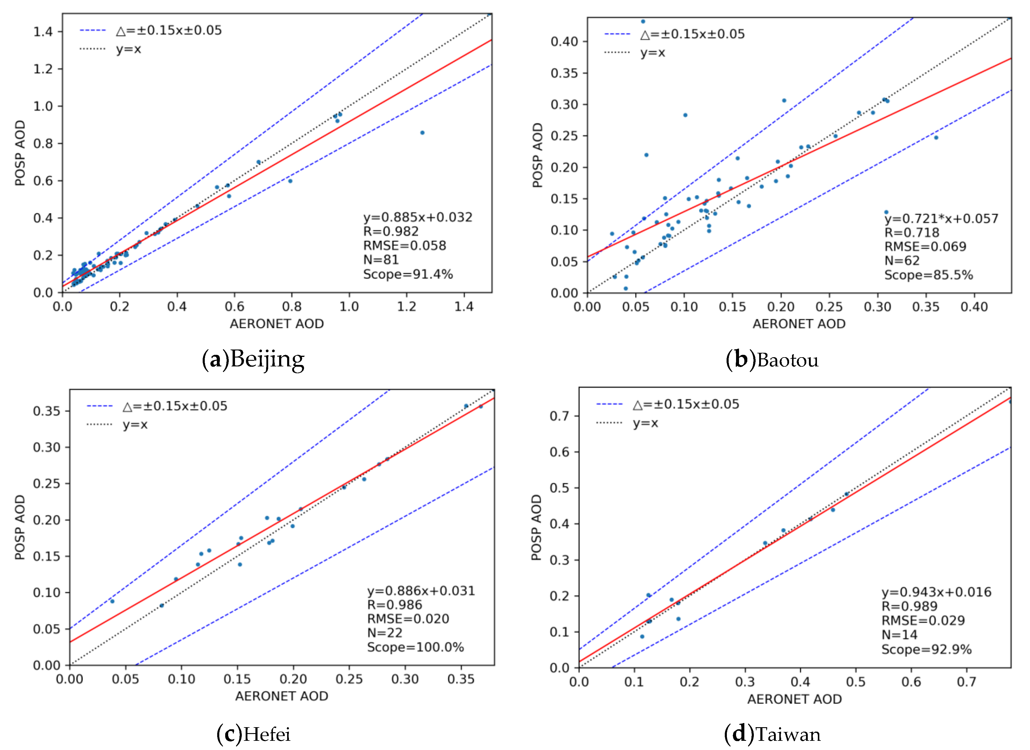
4.3. Validation against Ground-Based Data

The AERONET level 2.0 category is used for ground-based validation in this paper. AERONET is a ground-based network of sun photometers that provides high-quality aerosol measurements including AOD products [36,51].
The spectral AOD are retrieved using the proposed algorithm. With regard to validation, the AOD at 670 nm is selected. Correspondingly, the AOD at 675 nm in the AERONET products is used.
In order to verify the effectiveness of the inversion algorithms in different regions, four regions (Beijing, Hefei, Baotou, and Taiwan) with considerable geographical differences were selected. Additionally these four areas have AERONET ground-based long-term observation stations, namely: Beijing area (Beijing station), Baotou area (AOE_Baotou station), Hefei area (Hefei station) and Taiwan area (Chen-Kung_Univ station), the corresponding latitude and longitude are shown in Table 3.
The location and observation time of the AERONET sites are matched to extract the observation data corresponding to POSP from November 2021 to July 2022, as shown in Figure 4.
The validation against the corresponding AEROENT product is shown in Figure 5a–d are the verification results in Beijing, Baotou, Hefei and Taiwan, respectively.
It can be found from Figure 5 that the inversion results based on the algorithm proposed in this paper are basically consistent with AOD products of the AERONET sites, and the results are good. However, due to the influences of different surface types and aerosol types, the Scope is different. The order from largest to smallest is Hefei, Taiwan, Beijing, and Baotou. The reason for this may be that the surface vegetation in the Baotou area is sparse and is often considered to be a bright surface, while the Hefei site is mostly covered by evergreen vegetation, and the surface reflectance value is relatively small, so that the impact of the surface on the apparent reflectance is relatively smaller than the bright surface.
In addition, the aerosols in Baotou are mainly composed of coarse particles, so when polarization inversion is performed, the AOD obtained will have a large error, and then a large error will be introduced when the initial value of surface reflectance is provided based on the results of polarization inversion, resulting in relatively poor final inversion results.

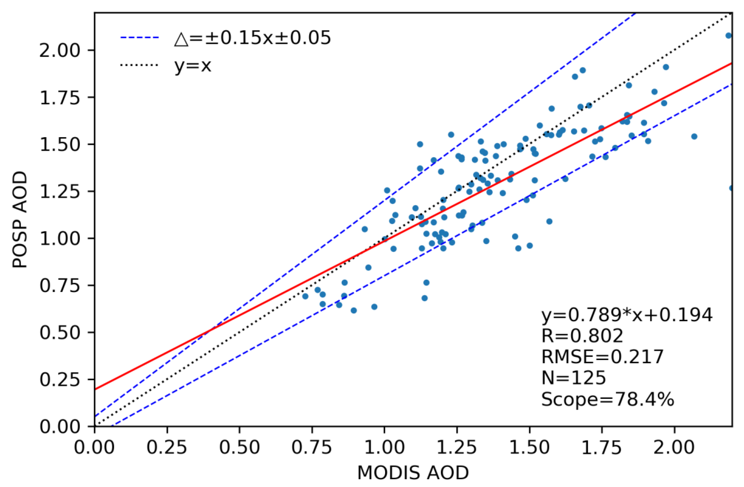
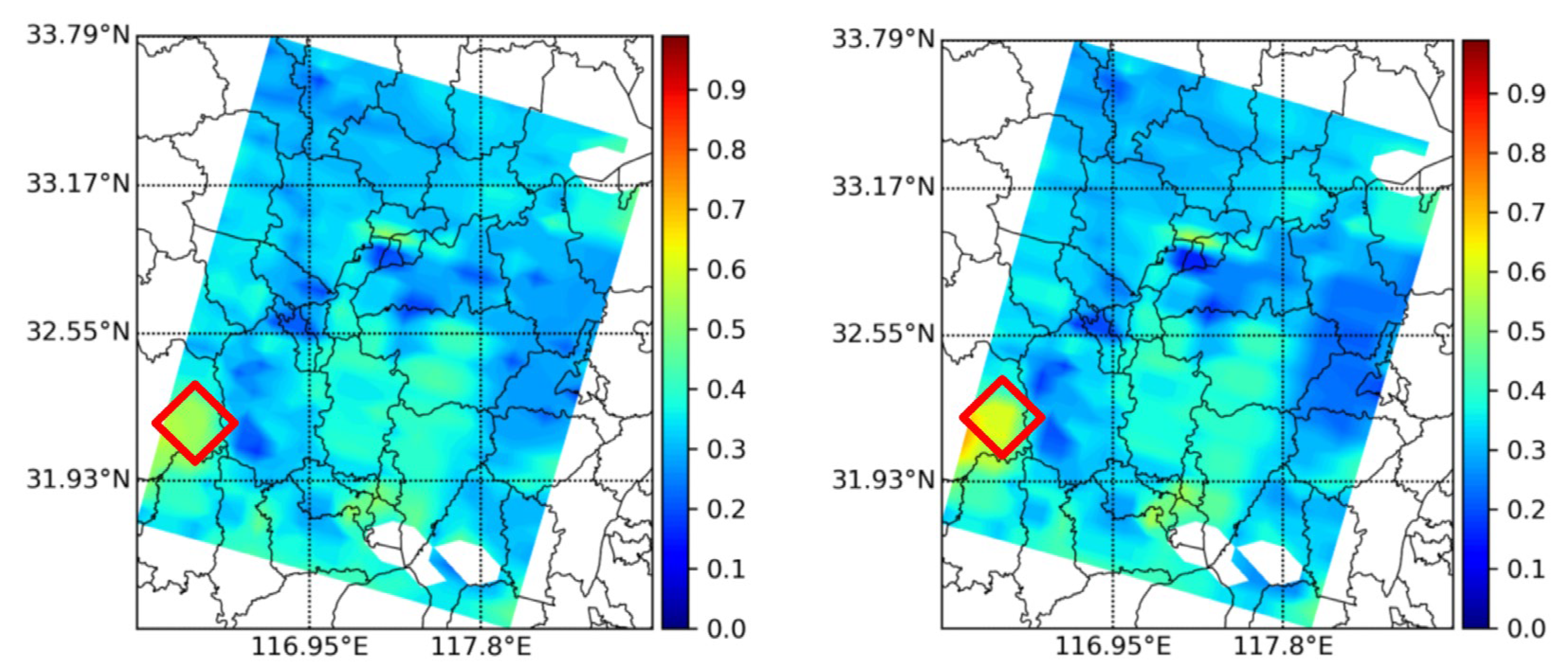
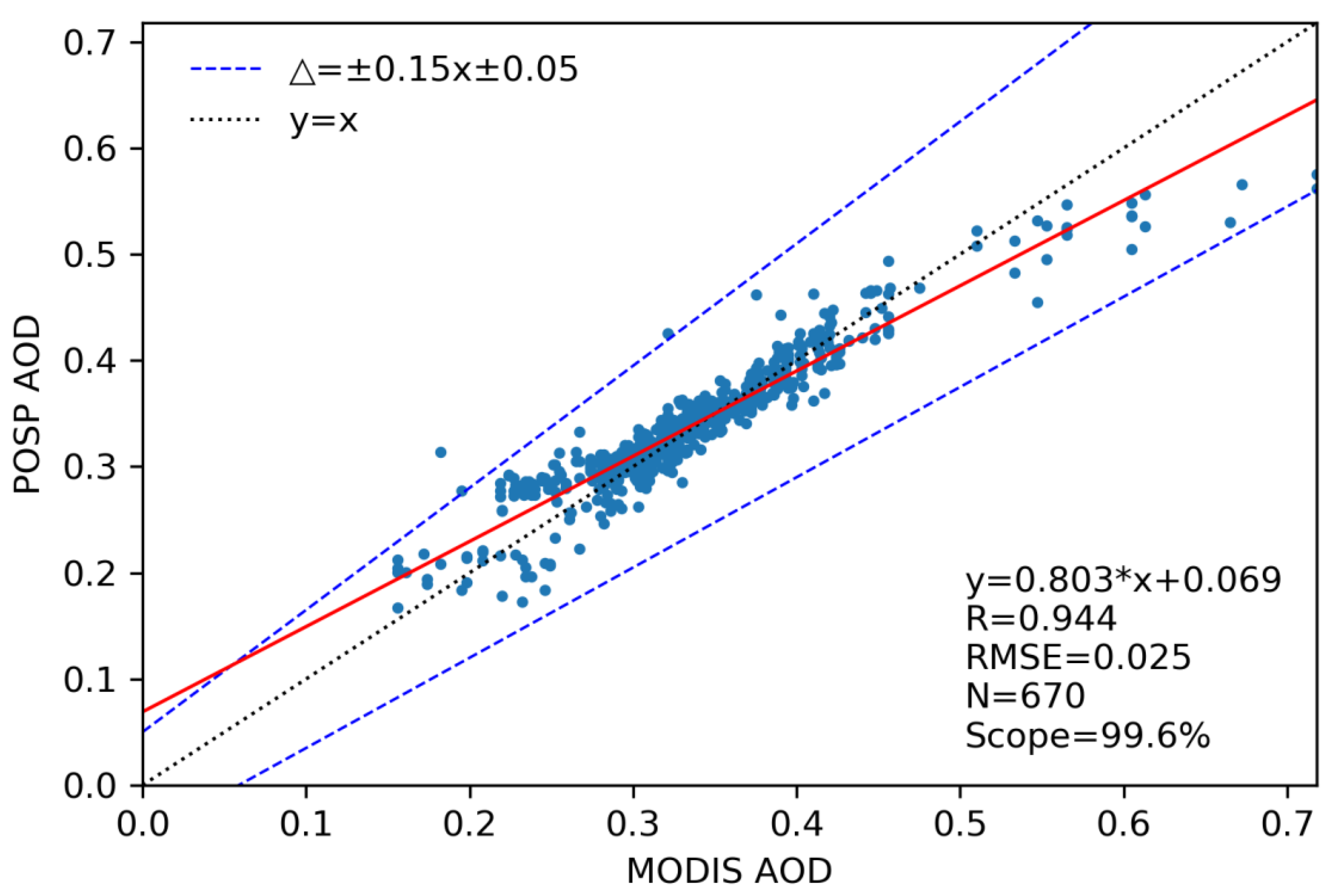
4.4. The Validation against MODIS Products

In order to verify the effectiveness of the intensity polarization joint inversion algorithm under different pollution conditions, MODIS’s AOD products at 550 nm are first used to screen the time and longitude ranges of AOD high value (AOD > 0.7) and low value (AOD < 0.7), and then filter out the corresponding POSP observation data. The specific latitude and longitude ranges and times are shown in Table 4.
The comparison between the inversion results in the high-value area and the MODIS product is shown in Figure 6. The blank area in the figure indicates no inversion results, because they are cloud pixels or no data.
Comparing the (a) and (b) figures in Figure 6, it can be found that the inversion results of POSP are consistent with the MODIS product as a whole, but that the inversion value of POSP in some areas is smaller than the AOD value in MODIS (prismatic area in the figure), and that the AOD value of POSP is greater than that of MODIS in some areas (circular area in the figure). In order to further analyze the difference between the AOD inversion results of POSP and the MODIS products, the inverted AOD and MODIS products were statistically analyzed and linear regression analysis was performed, and the results are shown in Figure 7.
According to the statistical results of Figure 7, a total of 125 high-value AOD data are obtained, of which 78.4% of the data fall within the error range, and the correlation coefficient R is 0.802.
Figure 8 shows the comparison of the AOD inversion results of POSP in the low AOD value area with the MODIS product. Comparing (a) and (b), it can be found that the POSP inversion results are consistent with the MODIS product as a whole. In some areas, the inversion result of POSP is smaller than MODIS (the prismatic area in the figure). In order to further analyze the effectiveness of the inversion algorithm, the inversion results and MODIS products were statistically analyzed, and the results are shown in Figure 9.
As can be seen from Figure 9, a total of 670 data points are obtained, 99.6% of the data are within the error range, and the correlation coefficient R is 0.944, indicating that the inversion results are in good agreement with the MODIS.
In summary, comparing the inversion results of high-value AOD and low-value AOD, it can be found that the inversion results of low-value AOD are significantly better than those in high-value AOD regions. This may be due to the assumption that the 2250 nm band is not sensitive to the atmosphere when performing polarization inversion, so that the TOA polarization reflectance of 2250 nm is used as the surface polarization reflectance of other bands. When the AOD is low, this assumption may have little effect on the inversion results, but in the high AOD value region, due to the increased probability of collision between light and particles, the 2250 nm band will carry more aerosol information, which will have a certain impact on the inversion results.

5. Conclusions

In this paper, based on the observation characteristics of POSP single-angle multi-band polarization measurements, an intensity polarization joint optimization inversion algorithm based on optimization theory is proposed, which can effectively perform ground-air decoupling without prior knowledge of the surface. Additionally, the effectiveness of the algorithm is verified in different regions and under different pollution conditions. It is found that in the vegetation coverage area (Hefei) and the urban underlying surface (Beijing and Taiwan), the correlation coefficient between the inversion AOD at 670 nm from POSP and the ground-based AOD at 675 nm from AERONET can reach more than 0.98. Good results can also be obtained on the bright surface (Baotou), the correlation coefficient can reach 0.71, and the proportion of data within the error range can reach 85.5%. In addition, the inversion results of the high-value area and the low-value area of AOD are also analyzed. It is found that the AOD at a 550 nm correlation coefficient between POSP and MODIS in the high-value area is 0.802, and in the low-value area, it is 0.994, indicating that the performance of the algorithm in the low-value area is better than that of the high-value area.
This algorithm uses the insensitivity of the short-wave infrared band to the atmosphere to obtain the initial value of the surface polarized reflectance. Therefore, in the high-value area of aerosol or under the condition coarse mode dominated aerosol, it will have a certain impact on the inversion results.

Author Contributions

Formal analysis, Y.F.; Funding acquisition, X.S.; Methodology, Y.F.; Project administration, X.S.; Supervision, X.S.; Validation, Y.F.; Writing—original draft, Y.F.; Writing—review and editing, X.S., R.T., H.H., X.L. and H.Y. All authors have read and agreed to the published version of the manuscript.

Funding

This work was supported by the Aerospace Science and Technology Innovation Application Research Project (E23Y0H555S1), the China High-resolution Earth Observation System (CHEOS) (30-Y20A010-9007-17/18), and the China Center for Resource Satellite Data and Applications Project (E13Y0J31601).

Data Availability Statement

Not applicable.

Acknowledgments

We are very grateful to Jun Wang and Xiaoguang Xu for the UNL-VRTM radiative transfer code. The data and FORTRAN codes used for the forward simulations are available on the UNL-VRTM website. We would like to thank all the relevant principal investigators and their staff for establishing and maintaining the AERONET stations used in this study. We are extremely grateful to the researchers of MODIS data products.

Conflicts of Interest

The authors declare no conflict of interest.

References

  1. Boucher, O.; Anderson, T.L. General circulation model assessment of the sensitivity of direct climate forcing by anthropogenic sulfate aerosols to aerosol size and chemistry. J. Geophys. Res. Atmos. 1995, 100, 26117–26134. [Google Scholar] [CrossRef]
  2. Haywood, J.; Boucher, O. Estimates of the direct and indirect radiative forcing due to tropospheric aerosols: A review. Rev. Geophys. 2000, 38, 513–543. [Google Scholar] [CrossRef]
  3. Satheesh, S.; Moorthy, K.K. Radiative effects of natural aerosols: A review. Atmospheric Environ. 2005, 39, 2089–2110. [Google Scholar] [CrossRef]
  4. Pincus, R.; Baker, M.B. Effect of precipitation on the albedo susceptibility of clouds in the marine boundary layer. Nature 1994, 372, 250–252. [Google Scholar] [CrossRef]
  5. Tao, W.-K.; Chen, J.-P.; Li, Z.; Wang, C.; Zhang, C. Impact of aerosols on convective clouds and precipitation. Rev. Geophys. 2012, 50. [Google Scholar] [CrossRef] [Green Version]
  6. Stevens, B.; Feingold, G. Untangling aerosol effects on clouds and precipitation in a buffered system. Nature 2009, 461, 607–613. [Google Scholar] [CrossRef] [PubMed]
  7. Christensen, M.W.; Jones, W.K.; Stier, P. Aerosols enhance cloud lifetime and brightness along the stratus-to-cumulus transition. Proc. Natl. Acad. Sci. USA 2020, 117, 17591–17598. [Google Scholar] [CrossRef]
  8. Fan, J.; Wang, Y.; Rosenfeld, D.; Liu, X. Review of aerosol–cloud interactions: Mechanisms, significance, and challenges. J. Atmos Sci. 2016, 73, 4221–4252. [Google Scholar] [CrossRef]
  9. Seaton, A.; Godden, D.; MacNee, W.; Donaldson, K. Particulate air pollution and acute health effects. Lancet 1995, 345, 176–178. [Google Scholar] [CrossRef]
  10. Kaufman, Y.J.; Tanré, D.; Boucher, O. A Satellite View of Aerosols in the Climate System. Nature 2002, 419, 215–223. [Google Scholar] [CrossRef]
  11. Li, Z.; Niu, F.; Fan, J.; Liu, Y.; Rosenfeld, D.; Ding, Y. Long-term impacts of aerosols on the vertical development of clouds and precipitation. Nat. Geosci. 2011, 4, 888–894. (In English) [Google Scholar] [CrossRef]
  12. Ramanathan, V.; Crutzen, P.J.; Lelieveld, J.; Mitra, A.P.; Althausen, D.; Anderson, L.M.; Andreae, M.; Cantrell, W.; Cass, G.R.; Chung, E.; et al. Indian Ocean Experiment: An integrated analysis of the climate forcing and effects of the great Indo-Asian haze. J. Geophys. Res. Atmos. 2001, 106, 28371–28398. (In English) [Google Scholar] [CrossRef]
  13. Hoek, G.; Krishnan, R.M.; Beelen, R.; Peters, A.; Ostro, B.; Brunekreef, B.; Kaufman, J.D. Long-term air pollution exposure and cardio- respiratory mortality: A review. Environ. Health 2013, 12, 43. [Google Scholar] [CrossRef] [Green Version]
  14. Zhang, Y.; Li, Z. Remote sensing of atmospheric fine particulate matter (PM2.5) mass concentration near the ground from satellite observation. Remote Sens. Environ. 2015, 160, 252–262. (In English) [Google Scholar] [CrossRef]
  15. Song, C.; He, J.; Wu, L.; Jin, T.; Chen, X.; Li, R.; Ren, P.; Zhang, L.; Mao, H. Health burden attributable to ambient PM2.5 in China. Environ. Pollut. 2017, 223, 575–586. [Google Scholar] [CrossRef]
  16. Hauser, A.; Oesch, D.; Foppa, N.; Wunderle, S. NOAA AVHRR derived aerosol optical depth over land. J. Geophys. Res. Atmos. 2005, 110. [Google Scholar] [CrossRef]
  17. Li, C.; Lau, A.K.H.; Mao, J.; Chu, D.A. Retrieval, validation, and application of the 1-km aerosol optical depth from MODIS measurements over Hong Kong. IEEE Trans. Geosci. Remote Sens. 2005, 43, 2650–2658. [Google Scholar] [CrossRef]
  18. Li, L.; Yang, J.; Wang, Y. An improved dark object method to retrieve 500m-resolution AOT (Aerosol Optical Thickness) image from MODIS data: A case study in the Pearl River Delta area, China. ISPRS J. Photogramm. Remote Sens. 2014, 89, 1–12. [Google Scholar] [CrossRef]
  19. Mei, L.L.; Xue, Y.; Kokhanovsky, A.A.; von Hoyningen-Huene, W.; de Leeuw, G.; Burrows, J.P. Retrieval of aerosol optical depth over land surfaces from AVHRR data. Atmospheric Meas. Technol. 2014, 7, 2411–2420. [Google Scholar] [CrossRef] [Green Version]
  20. Wei, J.; Huang, B.; Sun, L.; Zhang, Z.; Wang, L.; Bilal, M. A Simple and Universal Aerosol Retrieval Algorithm for Landsat Series Images over Complex Surfaces. J. Geophys. Res. Atmos. 2017, 122, 13338–13355. (In English) [Google Scholar] [CrossRef]
  21. Kaufman, Y.; Wald, A.; Remer, L.; Gao, B.-C.; Li, R.-R.; Flynn, L. The MODIS 2.1-μm channel-correlation with visible reflectance for use in remote sensing of aerosol. IEEE Trans. Geosci. Remote Sens. 1997, 35, 1286–1298. [Google Scholar] [CrossRef]
  22. Levy, R.C.; Remer, L.A.; Mattoo, S.; Vermote, E.F.; Kaufman, Y.J. Second-generation operational algorithm: Retrieval of aerosol properties over land from inversion of Moderate Resolution Imaging Spectroradiometer spectral reflectance. J. Geophys. Res. Atmos. 2007, 112, D13211. [Google Scholar] [CrossRef] [Green Version]
  23. Levy, R.C.; Remer, L.A.; Kleidman, R.G.; Mattoo, S.; Ichoku, C.; Kahn, R.; Eck, T.F. Global evaluation of the Collection 5 MODIS dark-target aerosol products over land. Atmos. Chem. Phys. 2010, 10, 10399–10420. (In English) [Google Scholar] [CrossRef] [Green Version]
  24. Hsu, N.C.; Tsay, S.-C.; King, M.D.; Herman, J.R. Aerosol Properties Over Bright-Reflecting Source Regions. IEEE Trans. Geosci. Remote Sens. 2004, 42, 557–569. (In English) [Google Scholar] [CrossRef]
  25. Hsu, N.C.; Tsay, S.-C.; King, M.D.; Herman, J.R. Deep Blue Retrievals of Asian Aerosol Properties During ACE-Asia. IEEE Trans. Geosci. Remote Sens. 2006, 44, 3180–3195. (In English) [Google Scholar] [CrossRef]
  26. Martonchik, J.V. Determination of aerosol optical depth and land surface directional reflectances using multiangle imagery. J. Geophys. Res. Atmos. 1997, 102, 17015–17022. [Google Scholar] [CrossRef]
  27. Martonchik, J.; Diner, D.; Kahn, R.; Ackerman, T.; Verstraete, M.; Pinty, B.; Gordon, H. Techniques for the retrieval of aerosol properties over land and ocean using multiangle imaging. IEEE Trans. Geosci. Remote Sens. 1998, 36, 1212–1227. [Google Scholar] [CrossRef] [Green Version]
  28. Diner, D.J.; Martonchik, J.V.; Kahn, R.A.; Pinty, B.; Gobron, N.; Nelson, D.L.; Holben, B.N. Using angular and spectral shape similarity constraints to improve MISR aerosol and surface retrievals over land. Remote Sens. Environ. 2005, 94, 155–171. [Google Scholar] [CrossRef]
  29. Deuzé, J.L.; Bréon, F.M.; Devaux, C.; Goloub, P.; Herman, M.; Lafrance, B.; Maignan, F.; Marchand, A.; Nadal, F.; Perry, G.; et al. Remote sensing of aerosols over land surfaces from POLDER-ADEOS-1 polarized measurements. J. Geophys. Res. Atmos. 2001, 106, 4913–4926. [Google Scholar] [CrossRef] [Green Version]
  30. Herman, M.; Deuzé, J.; Marchand, A.; Roger, B.; Lallart, P. Aerosol remote sensing from POLDER/ADEOS over the ocean: Improved retrieval using a nonspherical particle model. J. Geophys. Res. Atmos. 2005, 110. [Google Scholar] [CrossRef]
  31. Tanré, D.; Bréon, F.M.; Deuzé, J.L.; Dubovik, O.; Ducos, F.; François, P.; Goloub, P.; Herman, M.; Lifermann, A.; Waquet, F. Remote sensing of aerosols by using polarized, directional and spectral measurements within the A-Train: The PARASOL mission. Atmospheric Meas. Technol. 2011, 4, 1383–1395. [Google Scholar] [CrossRef] [Green Version]
  32. Bréon, F.; Vermeulen, A.; Descloitres, J. An evaluation of satellite aerosol products against sunphotometer measurements. Remote Sens. Environ. 2011, 115, 3102–3111. [Google Scholar] [CrossRef]
  33. Wang, H.; Sun, X.; Sun, B.; Liang, T.; Li, C.; Hong, J. Retrieval of aerosol optical properties over a vegetation surface using multi-angular, multi-spectral, and polarized data. Adv. Atmospheric Sci. 2014, 31, 879–887. (In English) [Google Scholar] [CrossRef]
  34. Fan, X.; Goloub, P.; Deuzé, J.-L.; Chen, H.; Zhang, W.; Tanré, D.; Li, Z. Evaluation of PARASOL aerosol retrieval over North East Asia. Remote Sens. Environ. 2008, 112, 697–707. [Google Scholar] [CrossRef]
  35. Dubovik, O.; Li, Z.; Mishchenko, M.I.; Tanré, D.; Karol, Y.; Bojkov, B.; Cairns, B.; Diner, D.J.; Espinosa, W.R.; Goloub, P.; et al. Polarimetric remote sensing of atmospheric aerosols: Instruments, methodologies, results, and perspectives. J. Quant. Spectrosc. Radiat. Transf. 2019, 224, 474–511. [Google Scholar] [CrossRef]
  36. Dubovik, O.; King, M.D. A flexible inversion algorithm for retrieval of aerosol optical properties from Sun and sky radiance measurements. J. Geophys. Res. Atmos. 2000, 105, 20673–20696. [Google Scholar] [CrossRef] [Green Version]
  37. Dubovik, O.; Lapyonok, T.; Litvinov, P.; Herman, M.; Fuertes, D.; Ducos, F.; Torres, B.; Derimian, Y.; Huang, X.; Lopatin, A.; et al. GRASP: A versatile algorithm for characterizing the atmosphere. SPIE Newsroom 2014, 25, 2–1201408. [Google Scholar] [CrossRef]
  38. Chen, X.; Yang, D.; Cai, Z.; Liu, Y.; Spurr, R.J.D. Aerosol Retrieval Sensitivity and Error Analysis for the Cloud and Aerosol Polarimetric Imager on Board TanSat: The Effect of Multi-Angle Measurement. Remote Sens. 2017, 9, 183. [Google Scholar] [CrossRef] [Green Version]
  39. Hou, W.; Wang, J.; Xu, X.; Reid, J.S. An algorithm for hyperspectral remote sensing of aerosols: 2. Information content analysis for aerosol parameters and principal components of surface spectra. J. Quant. Spectrosc. Radiat. Transf. 2017, 192, 14–29. [Google Scholar] [CrossRef]
  40. Hou, W.Z.; Li, Z.Q.; Zheng, F.X.; Qie, L.L. Retrieval of aerosol microphysical properties based on the optimal estimation method: Information content analysis for satellite polarimetric remote sensing measurements. In Proceedings of the ISPRS—International Archives of the Photogrammetry, Remote Sensing and Spatial Information Sciences, Beijing, China, 7–10 May 2018; pp. 533–537. [Google Scholar]
  41. Zheng, F.; Li, Z.; Hou, W.; Qie, L.; Zhang, C. Aerosol retrieval study from multiangle polarimetric satellite data based on optimal estimation method. J. Appl. Remote Sens. 2020, 14, 014516. [Google Scholar] [CrossRef]
  42. Yang, H.; Hong, J.; Zou, P.; Song, M.; Yang, B.; Liu, Z. Onboard Polarization Calibrators of Spaceborne Particulate Observing Scanning Polarimeter. Acta Optics Sinica. 2019, 39, 0912005. [Google Scholar] [CrossRef]
  43. Fan, Y.; Sun, X.; Ti, R.; Huang, H.; Liu, X. Information analysis of aerosol and surface parameters in PSAC observation over land. J. Infrared Millim. Waves 2022, 41, 15. [Google Scholar]
  44. Xu, X.; Wang, J. Retrieval of aerosol microphysical properties from AERONET photopolarimetric measurements: 1. Information content analysis. J. Geophys. Res. Atmos. 2015, 120, 7059–7078. [Google Scholar] [CrossRef] [Green Version]
  45. Rodgers, C.D. Inverse Methods for Atmospheric Sounding—Theory and Practice, Series on Atmospheric, Oceanic and Planetary Physics—Volume 2; World Scientific Publishing Co.: Singapore, 2000. [Google Scholar] [CrossRef] [Green Version]
  46. Fan, Y.; Sun, X.; Huang, H.; Ti, R.; Liu, X. The primary aerosol models and distribution characteristics over China based on the AERONET data. J. Quant. Spectrosc. Radiat. Transf. 2021, 275, 107888. [Google Scholar] [CrossRef]
  47. Wang, J.; Xu, X.; Ding, S.; Zeng, J.; Spurr, R.; Liu, X.; Chance, K.; Mishchenko, M. A numerical testbed for remote sensing of aerosols, and its demonstration for evaluating retrieval synergy from a geostationary satellite constellation of GEO-CAPE and GOES-R. J. Quant. Spectrosc. Radiat. Transf. 2014, 146, 510–528. (In English) [Google Scholar] [CrossRef] [Green Version]
  48. Waquet, F.; Léon, J.-F.; Cairns, B.; Goloub, P.; Deuzé, J.L.; Auriol, F. Analysis of the spectral and angular response of the vegetated surface polarization for the purpose of aerosol remote sensing over land. Appl. Opt. 2009, 48, 1228–1236. [Google Scholar] [CrossRef] [PubMed]
  49. Vermote, E.; Tanre, D.; Deuze, J.L.; Herman, M.; Morcrette, J.J. Second Simulation of the Satellite Signal in the Solar Spectrum (6S). 6S User Guide Version 2. Appendix III: Description of the subroutines. IEEE Trans. Geosci. Remote Sens. 1997, 35, 675–686. [Google Scholar] [CrossRef] [Green Version]
  50. Waquet, F.; Cairns, B.; Knobelspiesse, K.; Chowdhary, J.; Travis, L.D.; Schmid, B.; Mishchenko, M. Polarimetric remote sensing of aerosols over land. J. Geophys. Res. Atmos. 2009, 114, D1. [Google Scholar] [CrossRef]
  51. Dubovik, O.; Smirnov, A.; Holben, B.N.; King, M.D.; Kaufman, Y.J.; Eck, T.F.; Slutsker, I. Accuracy assessments of aerosol optical properties retrieved from Aerosol Robotic Network (AERONET) Sun and sky radiance measurements. J. Geophys. Res. Atmos. 2000, 105, 9791–9806. (In English) [Google Scholar] [CrossRef]
Figure 1. The size distribution of 8 aerosol models ([46]).
Remotesensing 15 00385 g001
Figure 2. The flowchart of inversion algorithm.
Remotesensing 15 00385 g002
Figure 3. (a,c) Illustrations of the iterative process for TOA reflectance and TOA polarized reflectance, respectively. (b,d) The plot of the cost function as a function of iterations in polarization inversion and intensity inversion, respectively (case for 8 June 2022).
Remotesensing 15 00385 g003
Figure 4. The flowchart of matching POSP observation data and AERONET data.
Remotesensing 15 00385 g004
Figure 5. Validation of the AOD at 670 nm with the proposed method against AOD at 675 nm in AERONET products at Beijing, Baotou, Hefei and Taiwan sites.
Remotesensing 15 00385 g005
Figure 6. POSP AOD inversion results (a) vs. MODIS products (b) (9 June 2022).
Remotesensing 15 00385 g006
Figure 7. The scatter plot of POSP AOD inversion results against MODIS products (9 June 2022).
Remotesensing 15 00385 g007
Figure 8. POSP AOD inversion results (a) vs. MODIS products (b) (4 May 2022).
Remotesensing 15 00385 g008
Figure 9. The scatter plot of POSP AOD inversion results against MODIS products (4 May 2022).
Remotesensing 15 00385 g009
Table 1. The basic parameters of POSP.
ParameterValue
Central wavelength/nm380, 410, 443, 490, 670, 865, 1380, 1610, 2250
Bandwidth/nm20, 20, 20, 20, 20, 40, 40, 60, 80
Stokes parametersI, Q, U
Quantized digit14 bit
Radiation calibration error≤5%
Polarization calibration error≤0.5%
Table 2. State vector x and observation vector y settings.
CategoryPolarization SettingIntensity Setting
Observation vector y = I p λ 1 , , I p λ 6 T                     y = I λ 1 , , I λ 7 T                                  
State vector x = V f , V c , ρ p T                                     x = V f , V c , ρ λ 1 , , ρ λ 7 T    
Table 3. AERONET data for validation.
AERONET SitesLongitude Latitude Date Range
Beijing116.381439.97692021.11–2022.7
AOE_Baotou109.628840.85172021.11–2022.7
Hefei117.162231.90472021.11–2022.7
Chen-Kung_Univ120.204722.99342021.11–2022.7
Table 4. Data information used for validation.
AOD RangeLongitude RangeLatitude RangeDate
AOD>0.7114.6–115.937.5–38.52022.6.9
AOD<0.7116.6–118.231.57–33.462022.5.4
Disclaimer/Publisher’s Note: The statements, opinions and data contained in all publications are solely those of the individual author(s) and contributor(s) and not of MDPI and/or the editor(s). MDPI and/or the editor(s) disclaim responsibility for any injury to people or property resulting from any ideas, methods, instructions or products referred to in the content.

