A New Approach for Feeding Multispectral Imagery into Convolutional Neural Networks Improved Classification of Seedlings

Abstract

Tree species information is important for forest management, especially in seedling stands. To mitigate the spectral admixture of understory reflectance with small and lesser foliaged seedling canopies, we proposed an image pre-processing step based on the canopy threshold (C_th) applied on drone-based multispectral images prior to feeding classifiers. This study focused on (1) improving the classification of seedlings by applying the introduced technique; (2) comparing the classification accuracies of the convolutional neural network (CNN) and random forest (RF) methods; and (3) improving classification accuracy by fusing vegetation indices to multispectral data. A classification of 5417 field-located seedlings from 75 sample plots showed that applying the C_th technique improved the overall accuracy (OA) of species classification from 75.7% to 78.5% on the C_th-affected subset of the test dataset in CNN method (1). The OA was more accurate in CNN (79.9%) compared to RF (68.3%) (2). Moreover, fusing vegetation indices with multispectral data improved the OA from 75.1% to 79.3% in CNN (3). Further analysis revealed that shorter seedlings and tensors with a higher proportion of C_th-affected pixels have negative impacts on the OA in seedling forests. Based on the obtained results, the proposed method could be used to improve species classification of single-tree detected seedlings in operational forest inventory.

1. Introduction

Classification of tree species is one of the key steps in remote sensing (RS)-based forest inventory to provide accurate estimates of structural characteristics of forests, such as species-specific tree densities and heights. However, it has been a challenging task for RS-based forest inventories [1], and it is an even more challenging in seedling stands [2], which are defined as homogenous forest stands in their early regeneration stages, i.e., with the mean height of dominating tree species being <7 or <9 m in coniferous or deciduous forests in Finland, respectively [3]. Therefore, new methods are needed in orderto improve the classification of seedlings. Seedling classification is challenging because the tree canopies in seedling stands often have lesser canopy foliage and variable canopy size. This is because some of the seedlings may have been planted while others—in Finland, often birches and other deciduous trees—are naturally regenerated within the same stand. This allows for a higher impact of reflectance from understory vegetation [4,5,6]. The seedlings may also be dense and even grow in thicket-like patterns, which causes mixed-canopy reflectance and hampers tree species classification. Therefore, this research aimed to introduce and explore a novel methodological approach to investigating the effect of tree height and foliage on species classification, explained as ecological factors that challenge the seedling species classification process.

RS technologies could support or replace field visits [7,8] carried out to collect the required information for the management of seedling stands. Such information includes tree species, height, and the number of trees per hectare (i.e., tree density). This information is needed in order to allocate tending and thinning operations in seedling forests, defined as the removal of competing understory vegetation and clustered and unwanted tree species from crop trees, respectively. This information plays a crucial role in assisting forest managers in the allocation of silvicultural operations, aiming at ensuring tree growth of the species of interest and future wood supply [3,9,10,11,12], as well as other ecological functions of seedling stands [13,14]; for example, it is important to give more growing space for coniferous seedlings than dominating and often unwanted deciduous seedlings [15] and understory [16,17], as deciduous seedlings, especially birches, outgrow coniferous seedlings during the early growth stages [15,18,19]. An RS-based forest inventory could collect the required information in a more spatially explicit and timely manner compared to field visits, which are considered to be time-consuming, costly, laborious, and often subjective.

Over the past few decades, several approaches to species classification have utilized machine learning. These approaches can be grouped into supervised, semi(weakly)-supervised, and unsupervised methods, all of which have been widely used in different forest RS tasks [1,20,21]. In particular, the random forest (RF) classifier and the rather-new deep learning methods (particularly convolutional neural networks (CNNs)) have been extensively utilized in tree species classification [21,22]. RF is an ensemble learning method that works by building several uncorrelated and independent decision trees, which predict the target response (i.e., species class [23]). It averages the probabilistic prediction of each class from the decision trees [24]. On the other hand, CNNs are based on a network of connected processing units organized in layers of intercorrelated nodes. The input images are converted to new feature maps based on a set of weights and biases applied in each layer [25]. In the simplest form, the data flow through each convolutional layer and pass forward to the next layer. Finally, a decision (species class) is made based on the values produced by the last layer [25,26,27]. In theory, a CNN is able to automatically extract relevant features and employ them in its own automatic manner during training with the least prior knowledge of the given task [28,29]. This is in contrast to traditional or conventional methods, such as RF, which usually require users to provide the features used in the classification task [30]. Using CNNs for classifying tree species in mature forests has been studied with different inputs of red–green–blue (RGB) and multi- and hyper-spectral data acquired from drone, air-, and space-borne RS platforms (e.g., [31,32,33,34,35]). CNNs have proven to be more accurate tree-classifiers than RF in different conditions, such as in mature forests [30,33] and urban or suburban environments [36,37]. However, the feasibility of CNNs compared to RF is still not understood in seedling stands where forest structure is complex due to different canopy sizes, canopy foliage cover percentages, and densely and unevenly located canopies. Only a few studies applied CNNs in mapping and attribute derivation in seedling trials; for example, Pearse et al. [38] and Hartley et al. [39] used a CNN for detecting seedlings, and estimating their heights in forestry seedling trials, respectively. However, these studies were conducted in trial forest conditions. There are numerous gaps in our knowledge related to the capabilities of CNN methods in the real-world operational management of seedling stands using low-cost operational multispectral drone (a.k.a., unmanned aerial vehicle (UAV)) data. Hence, it is an open question as to whether CNNs could classify seedlings more accurately compared to the RF classifier. Based on recent literature published on this matter, only two seedling studies carried out in real forest conditions used CNNs and drone-imagery. The first of these used a CNN to delineate and assess the height of seedlings in leaf-off conditions [40]; whereas the latter utilized a CNN for separating coniferous seedlings from non-seedling objects [41]. Hence, the use of multispectral drone imagery and CNNs to classify seedlings in real-forest conditions remains an unexplored topic; although Imangholiloo et al. [2] classified individual seedlings into spruce, birch, and non-tree classes using the intensity of multispectral airborne laser scanning (mALS) data via RF, the performance of RF on multispectral drone imagery with higher species classes needs more exploration.

The applied methodological improvement in this study—using canopy threshold (C_th)-based image pre-processing prior to feeding to CNN classifiers—was inspired by other seedling studies using ALS data. The studies usually applied C_ths between 0 and 1 m for the removal of laser returns from understory/ground [2,10,42,43,44,45]. C_ths between 0.5 and 1 m were also applied in seedling classification using conventional classifiers such as RF on hyper- or multi-spectral data [46]. However, the use of a C_th is a novel pre-processing option for CNNs, which has not been explored for tree species classification in seedlings or even mature trees. Furthermore, CNNs have not been compared against RF in seedling classification. Hence, this research aims to address the following research questions:

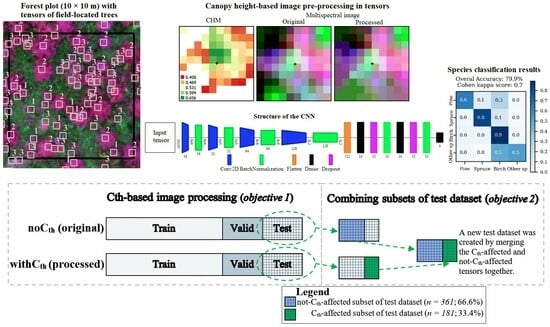
• Can the species classification accuracy of seedlings be improved by applying a C_th-based image pre-processing prior to feeding the CNN and RF classifiers?
• Can the species classification accuracy be improved when a new dataset is created by merging the C_th-affected and not-C_th-affected tensors together?
• Can CNN yield a more accurate seedling species classification accuracy than RF due to its higher capability of representing nonlinearity?
• Can species classification be improved by adding vegetation indices (VIs) into multispectral data in CNNs?

Moreover, the effects of the number of C_th-affected pixels and the height of seedlings on the classification accuracy were analyzed and discussed.

2. Materials and Methods

2.1. Study Area and Field Data Collection

The study area is located in Evo, southern Finland (61.20°N, 25.08°E (Figure 1)). The area consists of a forested area of ~2000 ha, with elevation varying from 125 m to 185 m above sea level. The forests in the Evo area are characterized by typical southern boreal forest conditions. Scots pine (Pinus sylvestris L.) and Norway spruce (Picea abies (L.) H. Karst.) are the dominant tree species in the area, whereas deciduous species comprise approximately one fifth of the total stem volume. Silver birch (Betula pendula Roth.) and white birch (Betula pubescens Ehrh.) are the main deciduous tree species in the area.

The field data were collected from 75 square shaped (10 × 10 m) sample plots that were placed on seedling stands within the study area. At first, existing forest resource information was used to determine stands that were classified as seedling stands within the study area. The existing forest resource information was used to classify the stands in different strata based on the main tree species and seedling density of the stand. Then, stratified sampling of seedling stands was performed by selecting a subsample from each seedling stand stratum to cover the whole variation of tree species classes and different seedling densities of the seedling stands on the study area. In total, 14 stands were selected to represent the whole variation of seedling stands. Then, the number of plots created on each stand was determined so that all the species classes and different seedling density classes were represented in the data. The field work was performed on these stands. For the collection of RS data, five data collection zones were created. Each of these zones covered approximately 10 ha.

During the field work, 75 sample plots were placed on the stands. On each stand, the longest intersecting line through the stand was created, and the sample plots were placed along it. The interval between the plots along the line was dependent on the area and shape of the stand. An additional line was created abeam of the intersecting line if the field crew noticed that it was not possible to place enough plots along the intersecting line due to the shape of the stand or other factors causing the rejection of any predefined sample plot locations. The starting point for the additional line was always one of the existing sample plot locations. The plot interval was fixed within the whole stand.

In the field, the field crew determined the direction of the line and the location of the plot center using a magnetic compass and measurement tape. If the structure of the forest was not representative of the stand in general, or the pre-defined plot had lots of variation within, the field crew was instructed to move the plot center to a location where the structure was more homogeneous and similar to the rest of the seedling stand area. The plot center was marked on the field and its location was determined with a real-time-kinematic (RTK) global navigation satellite system (GNSS) measurement (Trimble R2 and TSC7).

All trees located inside the 10 × 10 m plot and exceeding the height of one meter were tallied. Tree species were determined, and tree height was measured either by using a measurement stick or an electrical clinometer (Vertex IV, Haglöfs, Stockholm, Sweden). The use of the measurement device depended on the size of the tree. The location of each tree was determined by placing the receiver pole in an upright position as close as possible to the stump of the tree. Finally, the location was defined as an average of three RTK measurements, with an average horizontal error of 1.8 cm.

During the early development phase of a forest stand, there are typically several thickets of mainly deciduous saplings. In this study, these thickets were located with the RTK as one thicket in the measurements because it would not be possible to extract all the unique saplings belonging to the thickets from the RS data and measure their location with the RTK accurately. However, if the sapling thickets exceeded one meter in height, the number of unique individuals forming the thickets and their tree species were recorded.

A total of 5417 trees, including pine (13.6%), spruce (28.7%), birch (48.4%), and other species (9.3%), were measured inside the 75 plots. The other species class included rowan (Sorbus aucuparia L., 45.8%), willow (Salix spp., 30.5%), aspen (Populus tremula L., 17.5%), grey alder (Alnus incana L., 5.2%), juniper (Juniperus communis L., 0.6%), and larch (Larix sibirica Ledeb., 0.4%).

2.2. Remote Sensing Data

RS data acquisition was carried out using a quadcopter drone Geocopter X4 built by Videodrone Oy. The drone was equipped with post-processed kinematic (PPK)-level GNSS positioning technology.

The camera payload of the drone included two RGB and MicaSense (Seattle, WA, USA) multispectral cameras. Cameras were synchronized to capture images exactly at the same time to avoid any perspective differences between RGB and multispectral results, as well as with the PPK GNSS system to enable precise direct georeferencing.

The MicaSense multispectral camera was integrated with a light metering sensor DLS (downwelling light sensor), which was used in data processing to compensate for illumination differences between images within one flight. The MicaSense camera kit 50% reflectance panel was applied for each flight to set the right level for reflectances.

Drone images were collected during two days in five separate flights (

Table 1. Summary of remote sensing data used for this study. FWHM: full width at half maximum; GSD: ground sampling distance; RGB: red, green, blue; NIR: near-infrared.

	Multispectral Images	RGB Images
Name of Sensor	MicaSense MX Red-Edge	Sony A6000-series 24 Megapixel frame camera with 21 mm Voigtländer lens
Spectral bands	RGB, RedEdge, NIR	RGB
Central wavelength (nm)	475, 560, 668, 717, 840	-
FWHM (nm)	20, 20, 10, 10, 40	-
Resolution (GSD, cm)	5.5	1.3
Flight Altitude (m)	70	70
Drone speed (m/s)	8–9	8–9
Date	11 * and 15 ** September 2021	11 * and 15 ** September 2021
Time (UTC + 3)	12:30 to 14:30 * and 10:30 to 11:50 **	12:30 to 14:30 * and 10:30 to 11:50 **
Forward and side overlap (%)	80 and 75	85 and 80

* three flights; ** two flights.

). Weather conditions were cloudy or light overcast during both operating days. Due to the overcast conditions, both the DLS and the reflectance panels are recommended to be used in radiometric calibration by instructions of MicaSense. The panel was set to the ground for each flight corresponding to the lightning conditions during the flight by avoiding any shadows or distortions. Reference panel images were collected right before and right after each flight to obtain two baseline measurements with which to observe how the illumination conditions changed during the flight. DLS data were auto-saved to refer to illumination conditions of the individual image files.

2.3. Creating Dense Point Clouds and Orthomosaics

Image positions were initially estimated by employing the GNSS (Rinex) log data available from Trimble Virtual Reference Station (VRS) with the RTKLIB, version 2.4.3 b02 (www.rtklib.com, accessed on 10 October 2021) software. The initial positions of images were forwarded to a photogrammetric suite to find the accurate orientation and rotation of each image through photogrammetric adjustment. Photogrammetric processing was carried out with Agisoft Mestashape, version 1.7. Both camera datasets of each flight were processed separately.

The photogrammetric process included radiometric calibration and geometric calibration, in which image orientations and positions were accurately estimated. Afterwards, dense point clouds from RGB images and orthomosaics from multispectral data were created by employing adjusted parameters. The RGB camera system was geometrically calibrated earlier; therefore, no ground control point was used. The process of generating dense photogrammetric point clouds resulted in around 3 cm point distance (about 1400 points/m²). Orthomosaics were processed by applying a 3 m resolution DSM to avoid distortion of trees. Five-band multispectral orthomosaics were finally exported in 16-bit TIFF format.

2.4. Image Preprocessing

Canopy height models (CHMs) were created using drone photogrammetric point clouds (PPC) that were height-normalized using ground-classified laser returns of point clouds collected by a drone-based laser scanner (DJI Zenmuse L1 Lidar, Shenzhen, China). The flight was carried out on the 10 September 2021 at flight speed of 5 m/s and altitude of 55 m with planned point density of >700 points/m². The resolution of the CHM was 5 cm to match with multispectral data. The possible few null (empty) pixels in the CHM were filled using a 7 × 7 moving kernel over the null pixels only.

Next, we used a bounding box of 10 × 10 pixels (5 cm each pixel size, so it will be 50 × 50 cm as seedlings canopy) around the field-measured treetop location to create image data cubes (to call as tensors from now onward (Figure 1C)) for both classifiers identically. This dataset was created from the original multispectral data and called noC_th.

This step was followed by applying canopy threshold (C_th)-based image pre-processing on the noC_th dataset to minimize the effects of understory reflectance. This dataset is called withC_th. During the C_th-based image pre-processing, pixels of multispectral data were nullified if CHM values were ≤0.4 m. This step was followed by extracting handcrafted features for RF method and filling the nullified pixels by means of 8-closest pixels in a 3 × 3 moving kernel around the gap pixels for the CNN method. This gap-filling for tensors was needed for the CNN methods because they cannot handle the gaps yet. However, the gaps were not a problem for handcrafted features in RF because the features were at the tensor level. The noC_th dataset was created to be able to compare the effect of applying the proposed C_th-based image pre-processing method. The created noC_th dataset included all the same tensors as the withC_th dataset but no C_th-based images pre-processing was applied on them.

The introduced C_th-based image pre-processing method is depicted in Figure 2, with RGB for visual check (resolution 1.3 cm), CHM, the original tensors (i.e., noC_th dataset), and filled (after processing; withC_th dataset). The appearance of the colors of tensors become more homogenous.

2.5. Extracting Features for the Random Forest Classifier

Several spectral features (totaling 17, explained in

Table 2. A list of 17 extracted features from each band of multispectral data (MicaSense) from each tensor of 10 × 10 pixels (assuming it as a tree segment boundary).

Feature Name	Description of Features Meaning
Min	Minimum of reflectance within pixels of each tensor.
Max	Maximum of reflectance within pixels of each tensor.
Mean	Mean of reflectance within pixels of each tensor.
Stdev	Standard deviation of reflectance within pixels of each tensor.
Range	Range (Max-Min) of reflectance within pixels of each tensor.
Percentiles	Percentiles of the reflectance values of pixels of each tensor. Percentiles 10–90 (every 10%) and percentiles 5 and 95% were calculated, totaling 11 features.
NoData	Number of NoData pixels of each tensor which were omitted assuming as understory reflectance.

) were extracted from each band of MicaSense data of each tensor using Zonal Statistics in Python.

Next, eight vegetation indices (VIs) were calculated for each extracted feature of the tensors (

Table 3. List of vegetation indices (VIs) applied in this study with their equations.

	Full Name	Abbreviation	Equation
1	Normalized Difference Vegetation Index	NDVI	(NIR − Red)/(NIR + Red)
2	RedEdge NDVI	NDRE	(NIR − RedEdge)/(NIR + RedEdge)
3	Green NDVI	GNDVI	(NIR − Green)/(NIR + Green)
4	Simple ratio	SR	NIR/Red
5	NDVI times SR	NDVI × SR	NDVI × SR
6	Chlorophyll Vegetation Index	CVI	(NIR/Green) × (Red/Green)
7	Normalized Difference Greenness Index	NDGI	Green − Red/Green + Red
8	Difference Vegetation Index	DVI	NIR − Red

). The VIs and their equations are given in Table 3. This came to 221 features. The value of all handcrafted features (Table 2 and Table 3) in RF and tensors in the CNN methods were standard scaled.

2.6. Preparing Tensors for the Convolutional Neural Network Classifier

The input image tensors for the CNN contained a 3D shape of 10 (width) × 10 (height) × 5 (depth), including 500 floating point numbers. These tensors were used as training (80%), validating (10%), and testing (10%) sets for hyper-tuning inside a cross-validation (CV) process, while the testing data remained untouched until the end of this process.

Table 4. A summary of the number of training, validation, and test sets per each tree species class.

Species	Number (%) of Training Set	Number (%) of Validation Set	Number (%) of Test Set
Pine	579 (13.4%)	79 (14.6%)	81 (14.9%)
Spruce	1255 (29.0%)	150 (27.7%)	149 (27.5%)
Birch	2103 (48.5%)	258 (47.6%)	261 (48.2%)
Other species	396 (9.1%)	55 (10.1%)	51 (9.4%)
Total (5417)	4333 (80.0%)	542 (10.0%)	542 (10.0%)

shows the number of training, validation, and test sets of each species class used equally for both classifiers.

To address research question 4, a total number of 8 VIs (Table 3) were created and fused to the 5 bands of multispectral tensors to verify the importance of VIs in improving the overall accuracy. Therefore, the tensors of this analysis had a dimension of 10 (width) × 10 (height) × 13 (depth), yielding 1300 floating point numbers.

2.7. Training and Validation of the Random Forest Classifier

A 5-fold CV mechanism was employed using the grid_search functionality in the Scikit-learn library in Python [24] for hyper-tuning the training phase (i.e., training the RF with all possible combinations of given grid values of each parameter) and finding the RF with the highest validation accuracy (val_acc).

CV enables the examining of multiple values for each parameter of an estimator (RF).

Table 5. List of selected parameters for hyper-tuning inside grid_search CV with a short description, as well as the given list of values as input for the grid_search CV mechanism and the default values.

Parameter Name	Description (Pedregosa et al. [24])	Given Values for Grid	Default Value
max_depth	The maximum depth of the tree.	[None, 2, 10, 50, 80, 100]	None
min_samples_split	The minimum number of samples required to split an internal node.	[2, 3, 5, 8, 10, 12]	2 *
min_samples_leaf	The minimum number of samples required to be at a leaf node.	[1, 2, 3, 5, 20, 100]	1
max_features	The number of features to consider when looking for the best split **	[0, 2, ‘auto’, ‘log2’, ‘sqrt’, None]	sqrt
n_estimators	The number of trees in the forest. Usually, the bigger the better, but a larger number slows down the computation.	[75, 100, 125, 200, 500, 1000]	100

* Must be >1, gives error in 1. ** For classification usually “sqrt” is recommended, which is the default.

represents the selected parameters for hyper-tuning, their short description, our given list of values for the grid_search CV mechanism, as well as the default values.

N_estimators and max_features were the recommended main parameters for hyper-tuning, and the use of the CV method was underlined to find the best parameter values [24], the values in the default values for RF parameters, and more values around the defaults for hyper-tuning. This grid resulted in 7776 model combinations that were trained with 5-fold CV. Consequently, the best-trained model was selected out of 38,880 (7776 × 5) models.

For this CV step in RF, the training (80%) and validation sets (10%) were combined as input to grid_search, which splits the data into five and uses one split at a time for validation and the other four splits for training.

The most important features were analyzed from the CV-nominated best model, which had the highest val_acc. At this step, the features were sorted based on their importance (extracted from RF feature importance), and their intercorrelations with each other were checked. Finally, the five most important and not intercorrelated (<0.8) features were selected for training and predicting species classes. The same test dataset was used for both RF and the CNN.

2.8. Training and Validation of the Convolutional Neural Network

A sequential multi-layer perceptron (MLP) CNN was considered for this research by employing the Keras module [47], which is a part of the TensorFlow library [48]. In the sequential MLP CNN used in this research, an encoder segment with four convolutional blocks was considered, such that each convolution was followed by a batch normalization block. The encoder part was followed by a flatten block that vectorized the first two dimensions of its input tensor to fit into an MLP neural network. The architecture of the proposed network is depicted in (Figure 3) using Net2Vis v.3.18.3 software [49].

Figure 3 illustrates the structure of the CNN architecture. After obtaining the input tensors, the first Conv2D layer applies 16 random spatial convolutions over the input tensor shaped 10 × 10 × 5 (in noVIs, but 13 in withVIs), followed by batch normalization which normalizes the data such that they have a mean output of zero and a standard deviation of 1 [47]. These two steps—Conv2D and batch-normalization—are repeated three times, resulting in an output tensor of size 2 × 2 × 128 (Figure 3; Appendix A). Next, a flattening operation is carried out to convert the input tensor of 2 × 2 × 128 to a flat 512 × 1 tensor. This step is followed by applying dense, dropout, and batch normalization twice before finishing with a dense layer that outputs the probability of the input belonging to each of the 4 species classes.

The dense layer is a fully connected layer, meaning that each neuron inside it receives values from all the neurons on the previous layer [27]. It passes a weighted sum of its input to an activation function as (activation (dot (kernel, input) + bias). The activation function, by default, is a piecewise linear transform; however, other activation functions, such as rectified linear unit (relu) or hyperbolic tangent (tanh), are accessible. To avoid overfitting, one strategy is to select a few random nodes and add accidental noise to them by employing dropout layers [50,51].

The relu activation function was used in the conv2D and dense layers, except the last dense layer, where the softmax activation function was considered. The Relu activation function also increases the nonlinearity of the CNN models [32,52]. The softmax activation function in the last layer calculates the probability of each tensor being classified for each outcome (four species classes); hence, it outputs a vector of 4 values representing the 4 species classes. Finally, the adaptive moment estimation (Adam) optimizer with default settings and categorical_crosssentropy loss function was used in model.compile() (i.e., for training the model). The default values were used in this study for all hyperparameters apart from the dropout rates, dense units, and batches sizes, which were hyper-tuned. A Python code was developed to construct a dictionary including all possible combinations (7350) from the below grid. The code recorded all possible combinations:

• Dropout rate 1 = [0.0, 0.2, 0.4, 0.6, 0.8];
• Dropout rate 2 = [0.0, 0.2, 0.4, 0.6, 0.8];
• Dense unit 1 = [10, 50, 100, 150, 200, 250, 300];
• Dense unit 2 = [10, 50, 100, 150, 200, 250, 300];
• Batch_size = [32, 64, 128, 256, 1024, 1500].

Next, an index-parallelized for-loop was used to run and hyper-tune all possible combinations of the considered grid for optimizing and hyper-tuning the CNN methods. The for-loop was indexed from 0 to 7350 then run in parallel on tasks of each 1000 combinations in a CPU node (tasks 0–1000, 1000–2000, 2000–3000, …, 6000–7500). This was implemented to make the training phase efficient. After experimenting with the optimal computation resources, each task was submitted to a single-node computing unit with 10 CPUs. Each task used around 40% of 10 CPUs. All model training was implemented using the computation nodes of the Puhti supercomputer provided by the CSC–IT Center for Science, Finland [53].

Considering that the maximum epoch number was 300 iterations, the total possible run of CNN could be up to 2,205,000 model runs, but it never reached this due to the early stop function that was employed in the callback function (i.e., if val_acc was not improved after 100 epochs, then the training was stopped). A customized callback function was used in order to (1) save the best model when improvement is observed (when validation accuracy of an epoch is more than the earlier epoch) and (2) provide an early stop function (with patience of 100; i.e., if a model does not see improvement of validation accuracy after 100 runs, it stops).

To address research question 1, both the CNN and RF classifiers were trained on both withC_th and noC_th datasets separately to predict the tree species classes of the test datasets. As for research question 2, the test datasets of both the noC_th and withC_th datasets were divided into C_th-affected and not-C_th-affected subdatasets. Next, the trained models were used to predict only the corresponding subset of the test set, meaning that the model trained using the withC_th dataset was used to predict the withC_th subset of the test dataset, and the model trained with the noC_th dataset was used to predict the noC_th subset of the test dataset (Figure 4). In this analysis, only the C_th-affected tensors (181 out of 542 test tensors (33.4%)) and the not-C_th-affected tensors (361 out of 542 test tensors (66.6%)) were used as subsets of the test datasets, and there was no need for re-running the classifiers, as the species classes were already predicted, and we just switched the predicted species classes for the subsets of the test dataset (Figure 4). In this analysis, it was hypothesized that the C_th-affected tensors (corresponding to shorter seedlings) could be classified more accurately in the withC_th dataset, and the not-C_th-affected tensors could be classified more accurately in the noC_th dataset because the classifiers could select the most suitable model parameter settings for each input dataset automatically. Figure 4 shows the idea in a schematic way.

To study research question 3, the species classification accuracies of RF and the CNN were compared. In addressing research question 4, the CNN models were trained on the noVIs dataset with only 5 multispectral bands (tensors shape 10 × 10 × 5) and the withVIs dataset with 8 additional VIs (10 × 10 × 13).

Of note, the random seed was set to be fixed in CNN using the following commands: np.random.seed(42), python_random.seed(42), tf.random.set_seed(42). Similarly, random_state = 42 in Scikit-learn was applied for RF. This was applied to obtain reproducible results and reduce the randomness of outputs.

2.9. Accuracy Assessments

The species classification was assessed via overall accuracy (OA), kappa coefficient, precision (a.k.a., positive predictive value or user accuracy for positives), recall (a.k.a., true positive rate or producer accuracy for positives), and F1 scores (Equations (1)–(5)):

$$\mathrm{O}\mathrm{A}=\frac{\mathrm{T}\mathrm{P}+\mathrm{T}\mathrm{N}}{\mathrm{T}\mathrm{P}+\mathrm{T}\mathrm{N}+\mathrm{F}\mathrm{P}+\mathrm{F}\mathrm{N}},$$

(1)

$$\mathrm{K}\mathrm{a}\mathrm{p}\mathrm{p}\mathrm{a}=\frac{2\times (\mathrm{T}\mathrm{P}\times \mathrm{T}\mathrm{N}-\mathrm{F}\mathrm{N}\times \mathrm{F}\mathrm{P})}{\left(\mathrm{T}\mathrm{P}+\mathrm{F}\mathrm{P}\right)\times \left(\mathrm{F}\mathrm{P}+\mathrm{T}\mathrm{N}\right)+\left(\mathrm{T}\mathrm{P}+\mathrm{F}\mathrm{N}\right)\times (\mathrm{F}\mathrm{N}+\mathrm{T}\mathrm{N})},$$

(2)

$$\mathrm{P}\mathrm{r}\mathrm{e}\mathrm{c}\mathrm{i}\mathrm{s}\mathrm{i}\mathrm{o}\mathrm{n}=\frac{\mathrm{T}\mathrm{P}}{\mathrm{T}\mathrm{P}+\mathrm{F}\mathrm{P}},$$

(3)

$$\mathrm{R}\mathrm{e}\mathrm{c}\mathrm{a}\mathrm{l}\mathrm{l}=\frac{\mathrm{T}\mathrm{P}}{\mathrm{T}\mathrm{P}+\mathrm{F}\mathrm{N}},$$

(4)

$$\mathrm{F}1=2\times \frac{\mathrm{P}\mathrm{r}\mathrm{e}\mathrm{c}\mathrm{i}\mathrm{s}\mathrm{i}\mathrm{o}\mathrm{n}\times \mathrm{R}\mathrm{e}\mathrm{c}\mathrm{a}\mathrm{l}\mathrm{l}}{\mathrm{P}\mathrm{r}\mathrm{e}\mathrm{c}\mathrm{i}\mathrm{s}\mathrm{i}\mathrm{o}\mathrm{n}+\mathrm{R}\mathrm{e}\mathrm{c}\mathrm{a}\mathrm{l}\mathrm{l}},$$

(5)

where TP is true positives, TN is true negatives, FP is false positive, and FN is false negatives.

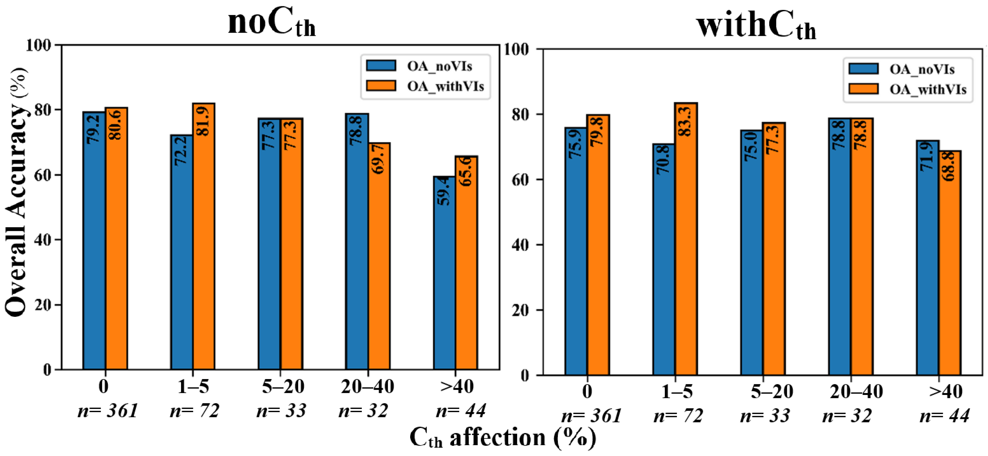
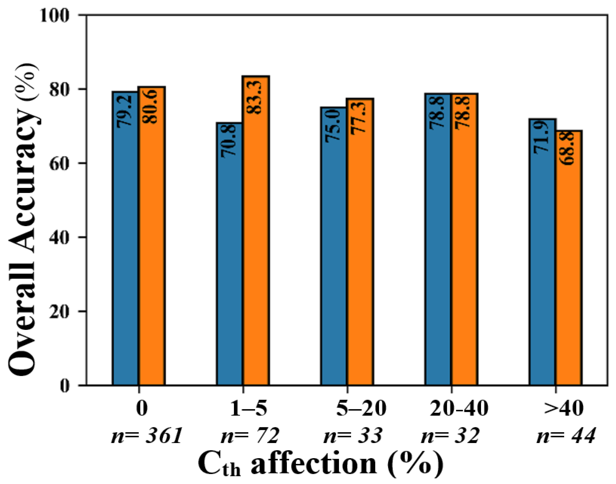
2.10. Analyzing the Effects of the Number of C_th-Affected Cells and Seedlings Height on Classification Accuracy

After obtaining the overall classification and accuracy assessments, the results were analyzed to explore the effects of the number of C_th-affected pixels on species classification, hypothesizing that C_th-affected tensors would be more accurately classified. For this, the test dataset (reference and predicted labels) was separated into 5 subsets of 1–5, 5–20, 20–40, and >40%. The uneven binning in these subsets was implemented to include a fair amount of (at least 30) data inside each bin. In fact, this binning process helps scratch the C_th-affected bins into four bins and retain the not-C_th-affected bins as one bin as a baseline. Considering the fact that the tensors had a dimension of 10 × 10 pixels (100 pixels), the numbers represent both real numbers and the percentages of C_th-affection rates per tensor.

The impact of seedling height on classification accuracy was also examined, assuming that smaller seedlings could be challenging for the classifiers (inspired by Imangholiloo 2020, 2021). The methodological improvement introduced in this research was expected to deal with the challenge. For this, the true and predicted labels of the test datasets were indexed by their field-measured height and grouped into 4 bins of seedling heights, namely, <1.5, 1.5–2, 2–4, and >4 m. To ensure the reliability of the results, the aim was to include at least 100 observations in each bin. The resulting bin counts were 150, 108, 172, and 112, respectively.

Finally, the accuracy assessment metrics presented Section 2.8 were used for all analyses.

3. Results

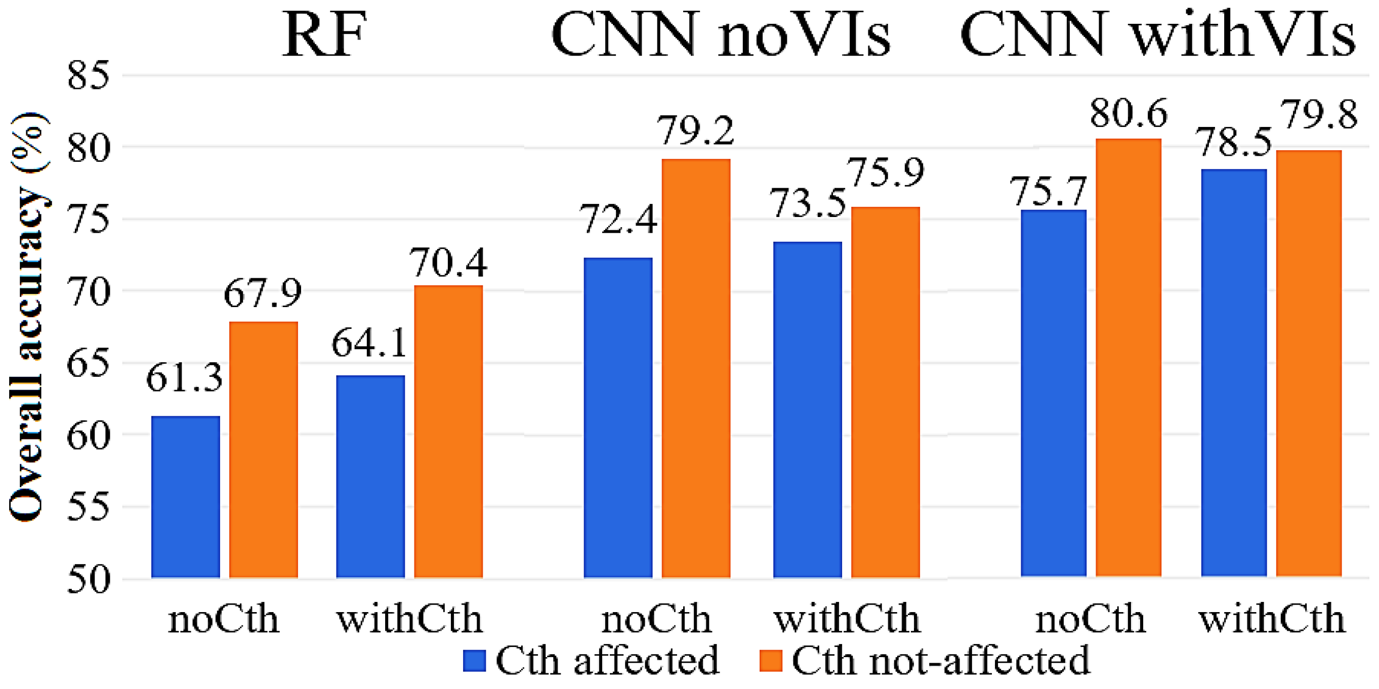
3.1. The Effects of Applying a Canopy Threshold (C_th) on the Accuracy of Species Classification in the CNN and RF Methods

Analyzing the C_th-affected (n = 181, 33.4%) and not-C_th-affected (n = 361, 66.6%) subsets of the test dataset in the noC_th and withC_th datasets revealed that the species classification accuracy was always improved in the C_th-affected subset of the test dataset when applying C_th-based image pre-processing (withC_th dataset) compared to when C_th was not applied (noC_th dataset). The species classification accuracy was increased from an OA of 75.7% to 78.5% before and after applying C_th-based image pre-processing in the CNN withVIs dataset (Figure 5). As for the classification accuracy within the not-Cth-affected subsets of the test dataset, the tree species classification was improved in RF (from an OA of 67.9% to 70.4%) in contrast to that classified via the CNN methods, which slightly declined (from an OA of 79.2% to 75.9% and from 80.6% to 79.8% in noVIs and with VIs, respectively).

To compare the results of fusing VIs in the CNN method, the species classification accuracy in the C_th-affected subset of the test dataset was improved from an OA of 72.4 to 73.5% and from 75.7% to 78.5% with regard to not fusing VIs (noVIs) and fusing VIs (withVIs) data to CNN, respectively. The amount of improvement was greatest with respect to fusing Vis (improved by 2.8 percentage points (pp)).

To compare the accuracy of two classifiers (CNN vs. RF), the results showed that the species classification accuracy was improved from 61.3% to 64.1% in RF, similar to the CNN noVIs (from 72.4% to 73.5%) and withVIs (from 75.7% to 78.5%). Hence, species classification was more accurate in the CNN compared to RF, in general.

Further analyzing the effects of the proportion of C_th-affection rates on the species classification accuracy (Figure 6) revealed that the species classification accuracy was highest at 1–5%-affections and lowest at >40%-affections in both noVIs and withVIs datasets. The OA varied from 59.4% to 79.2% in the noC_th dataset and from 70.8% to 78.8% in the withC_th noVIs dataset. Fusing VIs made the OA vary from 65.6% to 81.9% in noC_th and from 68.8% to 83.3% in withC_th (Figure 6).

Applying C_th-based image pre-processing improved the classification accuracy of seedlings on different Cth-affection rates; for example, when it was affected by over 40%, the OA was improved from 59.4% (noC_th) to 71.9% (withC_th) in the noVIs dataset, similar to that of withVIs (from 65.6% to 68.8%). As Figure 6 shows, the magnitude of improvement was highest at the tensors > 40% C_th-affected.

Seedling height was found to be another factor affecting the accuracy of species classification using CNNs. The OA was the highest (≥82%) for bins withC_th and withVIs if tree height was >1.5 m (bins of 1.5–2, 2–4, and >4 m) (Figure 7). For these bins, OA was also higher than the general OA (79.3%). The accuracy of species classification was lowest where seedlings were <1.5 m (which reached an OA of 60.0% at the highest in withVIs withC_th; Figure 7). The OA was lowest when seedlings were <1.5 m (OA = 58%) and highest at the tallest seedlings (>4 m, OA = 89.3%). Moreover, adding Vis improved the OA by 2, 5.6, 8.1, and 0.0 pp in the bins of <1.5, 1–2, 2–4, and >4 m, respectively. Thus, the highest improvement was when the seedling had a height of 2–4 m.

As Figure 7 shows, applying the C_th-based image classification improved the OA in the bin of <1.5 m from 56% to 58% (in noVIs) and in the bin of 1.5–2 m from 80.6% to 82.4% (withVIs).

Generally, employing C_th-based image pre-processing improved the OA from 67.9% to 68.3% in RF and from 79.0% to 79.3% in the CNN in the withVIs dataset (Figure 8). However, the OA slightly declined (1.8 pp, from 76.9% to 75.1%) in the noVIs dataset of CNN. Figure 8 summarizes the species classification accuracies using the two classifiers (RF and CNN) in the noC_th and withC_th datasets.

Comparing the performance of CNN with RF revealed that the CNN achieved a higher tree species classification accuracy compared to RF. The OA was at the lowest when using RF without C_th (67.9%), while it was boosted by 11.4 pp (to 79.3%) when using the CNN in the withC_th withVIs dataset. Moreover, fusing VIs improved the OA from 76.9% to 79.0% and from 75.1% to 79.3% in the noC_th and withC_th datasets when using the CNN method.

As for the species-specific classification accuracy, pines were more accurately classified with the CNN method (using both noVIs and withVIs) compared to RF. The recall of pines was 0.6 in CNN withVIs, while the recall for RF was only 0.3 (

Table 6. Evaluation of classification accuracy for each dataset and classifier (method) in the detailed metrics.

Dataset	Classifier	OA (%)	Kappa	Overall Precision (Per Species) *	Overall Recall (Per Species) *	Overall F1 Macro (Per Species) *	Overall F1 Micro
NoCth	RF	67.9	0.5	0.7 (0.5, 0. 7, 0.7, 1.0)	0.6 (0.3, 0.7, 0.8, 0.4)	0.6 (0.3, 0.7, 0.8, 0.6)	0.7
	CNN noVIs	76.9	0.6	0.8 (0.7, 0.8, 0.8, 0.8)	0.7 (0.6, 0.8, 0.9, 0.4)	0.7 (0.6, 0.8, 0.8, 0.5)	0.8
	CNN withVIs	79.0	0.7	0.8 (0.7, 0.9, 0. 8, 0.7)	0.7 (0.6, 0.8, 0.9, 0.5)	0.7 (0.7, 0.9, 0.8, 0.6)	0.8
WithCth	RF	68.3	0.5	0.7 (0.6, 0.7, 0.7, 0.8)	0.7 (0.3, 0.8, 0.8, 0.4)	0.6 (0.4, 0.7, 0.8, 0.5)	0.7
	CNN noVIs	75.1	0.6	0.7 (0.7, 0.8, 0.7, 0.7)	0.7 (0.6, 0.8, 0.8, 0.4)	0.7 (0.6, 0.8, 0.8, 0.5)	0.8
	CNN withVIs	79.3	0.7	0.8 (0.8, 0.8, 0.8, 0.8)	0.7 (0.6, 0.8, 0.9, 0.5)	0.7 (0.7, 0.8, 0.8, 0.6)	0.8
Combined dataset	RF	66.6	0.5	0.7 (0.6, 0.6, 0.7, 0.9)	0.5 (0.2, 0.7, 0.9, 0.4)	0.6 (0.3, 0.7, 0.8, 0.6)	0.7
	CNN noVIs	77.3	0.6	0.8 (0.7, 0.8, 0.8, 0.8)	0.7 (0.5, 0.8, 0.9, 0.4)	0.7 (0.6, 0.8, 0.8, 0.5)	0.8
	CNN withVIs	79.9	0.7	0.8 (0.8, 0.9, 0. 8, 0.7)	0.7 (0.6, 0.8, 0.9, 0.5)	0.7 (0.7, 0.9, 0.8, 0.6)	0.8

* The four numbers inside the parentheses show the accuracy metrics for each species of pine, spruce, birch, and other-species classes, respectively.

). Moreover, a significant fraction of other species were misclassified as birches in almost all the classifiers and datasets; for example, 40% of other species were misclassified as birch when using the CNN method on the withVIs withC_th dataset. The recall for RF and the CNN noVIs was even higher (0.6 in both), which caused a decline in the OA of species classification. Table 6 gives a detailed summary of the accuracy metrics.

3.2. The Effects of Combining the Subsets of the Test Dataset on the Accuracy of Species Classification in the CNN and RF Methods

Analyzing the effects of the C_th-affection rates on species classification accuracy (Figure 9) for the combined dataset revealed that the species classification accuracy in the withVIs dataset reached its highest value at 1–5%-affections (83.3%) and its lowest value at >40%-bin, similar to noC_th and withC_th dataset (Section 3.1). However, the OA in noVIs was highest at the 0% bin (79.2%) and lowest at the 1–5% bin (70.8%). Fusing VIs improved the OA of species classification in all bins (especially 1–5%-bin), except in the 20–40% bin, which did not change, and the >40% bin, which slightly declined (Figure 9).

Combining the subsets of the test dataset seemed to improve the OA of species classification by smartly selecting the subset of the dataset that was classified with higher accuracy. This can be observed in the different C_th-affection bins in Figure 9. Comparing Figure 6 and Figure 9 reveals that the more accurately classified subsets of the test dataset in each C_th-affection bin were selected in both noVIs and withVIs; for example, the OA in the combined dataset was 68.8% in the >40%-bin in the withVIs dataset. In fact, this number comes from the withC_th dataset of the same data (withVIs, Section 3.1). Because the OA in noC_th was 65.6%, and because it was improved to 68.8% in that bin, the consequence of combining the datasets would take that result. This smart selection of the higher accuracy resulted in the combined dataset having the same trend in all bins, even for the 0%-affected bins. For example, the OA was 80.6% in noC_th and 79.8% in withC_th in the 0% bin in the withVIs dataset, and as a result, it selected the higher accuracy (80.6%) in the combined method.

An analysis of the effect of seedling heights on the performance of species classification accuracy (another influential factor (Figure 10)) in the CNN in a combined method showed similar results as in the withC_th dataset (Section 3.1).

Overall (when not zooming to C_th-affection or seedling height), combining the C_th-affected and not-C_th-affected subsets of the test dataset improved the OA of species classification in the CNN methods; for example, the OA of species classification in CNN noVIs was improved from 76.9% (original, noC_th) and 75.1% (at withC_th) to 77.3% by employing the combined dataset. Similarly for CNN withVIs, it improved OA of species classification from 79.0% (noC_th, F micro: 0.8) and 79.3% (withC_th, F micro: 0.8) to 79.9% (F micro: 0.8). The amount of improvement was higher in the withVIs dataset (0.9 pp) compared to noVIs (0.3 pp). The same trend also exists when comparing the combined dataset with the withC_th dataset; for example, the OA improved from 75.1% in withC_th to 77.3% in the combined method on noVIs dataset, similarly to the withC_th dataset (which improved from 79.3% to 79.9%). The amount of improvement was greatest in the noVIs dataset (2.2 pp) compared to all others. However, the combined method did not improve the OA in RF (reached to 66.6%) compared to the noC_th (67.9%) and withC_th (68.3%) datasets. Figure 11 summarizes the species classification accuracies using the two classifiers (RF and CNN) in the combined dataset applied in this study.

The OA of species classification reached the highest values (79.9%) when applying the combined dataset in CNN and withVIs. Applying the combined method improved species classification accuracy in both CNN datasets (withVIs and noVIs).

When comparing the accuracy of the two classifiers (CNN vs. RF), CNN was the more accurate classifier compared to RF in the combined method too, similarly to that of C_ths when applied alone (Section 3.1). The OA of species classification of the combined method reached 66.6% in RF, while it was 77.3% and 79.9% in the CNN with the noVIs and withVIs datasets. Hence, the species classification was more accurate in CNN (up to 13.3 pp) compared to RF, in general. To compare the results when fusing VIs in the CNN method, the species classification accuracy was improved by up to 2.6 pp (from 77.3% to 79.9%) by fusing the VIs in CNN method in general.

Regarding the species-specific classification accuracy in the combined idea, the pine class was more accurately classified in the CNN method (using both noVIs and withVIs), compared to that in RF. More information is provided in Table 6.

3.3. Feature Importance in RF and Configurations of the Classifiers

The most important features in both datasets (noC_th and withC_th) were lower percentiles of NDGI (percentile 5 and 30 in noC_th and withC_th, respectively). These were followed by the higher percentile (90) of NDRE identically in both datasets (Figure 12). In the noC_th dataset, the standard deviation of NDRE, the 10th percentile of NDVI × S, and the standard deviation of band 4 were the following most important and uncorrelated features. The same (similar) features were selected for the withC_th dataset too, but they were only ranked/ordered differently.

According to the results, it seemed that NDRE was an important VI (used twice in both datasets (in percentile 90 and standard deviation)). Moreover, the redEdge band seemed important. In addition, there were many highly intercorrelated features that were dropped when checking whether the correlations were <0.8; for example, in the withC_th dataset, the following features were between the second (p90_NDRE) and third (std_b4) features: p30_NDRE (0.9); p80_NDRE (1.0); p5_NDGI (0.9); p60_NDRE (0.9); mean_NDRE (1.0); p20_NDGI (1.0); p50_NDRE (0.9); p40_NDGI (1.0); min_NDGI (0.8); p70_NDRE (1.0); p10_NDGI (1.0); p10_SR (0.8); max_NDRE (0.9). The features were sorted via RF importance, and the values in parentheses show the correlation with either the second or third selected feature.

As for the CNN models, the best validation accuracy was achieved in epochs 33 (val_acc: 80.8%) and 40 (val_acc: 81.6) using the withVIs dataset in noC_th and withC_th conditions, respectively. Appendix B presents a visualization of the training and validation accuracy in every epoch for the CNN models on the noC_th and withC_th datasets. The early-stop function in the callback stopped the models from running further if, after 100 epochs, val_acc was not increased. Moreover, the withC_th figure was less susceptible to overfitting due to a smaller difference between training and validation accuracy compared to that of noC_th (Appendix C), although both are acceptable and not susceptible to overfitting at all.

The CNN models created in this research have higher nonlinearity and are less (not) susceptible to overfitting; in fact, our CNN model is not overfitting due to the hyper-tuned dropout rate, which was set to 0.6 and 0.8 (Appendix C), as well as the fact that val_acc is not much different from test_acc. The difference between val_acc and test_acc in the CNN was even smaller than in RF. This indicates that our CNN models are not overfitting at all, with even less overfitting (if any) than RF.

4. Discussion

4.1. The Effects of Applying Canopy Threshold (C_th)-Based Image Pre-Processing on the Accuracy of Species Classification in CNN and RF

Improving seedling–tree species classification by employing C_th-based image pre-processing on input images prior to feeding to two classifiers—CNN and RF—was one of the main objectives of this research. Based on the results obtained in this research, the process improved the OA of species classification by up to 2.8 pp in the C_th-affected subset of the dataset in seedling forests. This could be attributed to minimizing the admixture of reflectance from the understory, especially in younger (shorter) seedlings (Figure 2).

To the best of the authors’ knowledge, the proposed methods have not been employed in seedling (or mature) stands. Hence, the results of this research could be discussed with respect to studies carried out in forests of different growing stages. An improvement of the OA of species classification between 1–4.3 pp was documented in mature forests by hybridizing the CNN and k-nearest neighbors [54], combining Res-Net and U-net structures [55], using their proposed 3D-1D-CNN method [56], and using a novel two-phase CNN [57]. Hence, the magnitude of improving the OA of classifying seedlings in this study was in line with the aforementioned literature of mature forests.

4.2. The Effects of Combining Subsets of Test Dataset on the Accuracy of Species Classification in CNN and RF

Creating a new dataset by merging C_th-affected and not-C_th-affected subsets of the test dataset further improved the accuracy of species classification; for example, it improved the OA of the C_th-affected tensors (33.4% of test set) by up to 2.8 pp (from 75.7% to 78.5%) in the CNN withVIs dataset. However, it slightly declined the OA in the not-C_th-affected tensors (from 80.6% to 79.8%). This was because the C_th-affected tensors of this study comprised only 33.4% of the dataset, and the rest of the data were not affected as their cells were all above the C_th of 0.4 m. It should be noted that apart from one of the forest plots in this study (1 of 75 plots), all of the plots were in advanced seedling (mean tree height > 1.3 m, AdS) stands, while in the study by Imangholiloo et al. [2], there were four plots in young seedling (mean tree height ≤ 1.3 m, YoS) stands plus ten plots in AdS. Hence, the methodology developed in this study could help in inventorying YoS more accurately, although it was documented to be challenging for characterizing seedling stands using hyperspectral and RGB photogrammetric point clouds [46] and using ALS [2,45].

The results of this study were in line with studies using a rather similar approach; for example, Martins et al. [58] developed a rather similar—albeit a post-processing—step in a multitask CNN (DeepLabv3⁺ with Res-Net backbone) based on combining the two outputs of the multitask CNN—semantic segmentation (labeled images) and regression outputs—for each image (a regression branch showing a distance map transform). They achieved an improvement of species classification to average F-score of 79.3 ± 8.6% in classifying tropical urban trees in Brazil. Similarly, Anderson et al. [59] achieved a higher OA when combining CNN and OBIA methods (91%) than when using CNN alone (88%) for the classification of an invasive species in wetlands using drone-based RGB imagery.

Unlike in the CNN, combining subsets of the test dataset to create a new dataset was not successful in RF based on our results. This could be attributed to the fact that the nullified pixels in the withC_th dataset were not filled because filling was not needed due to the nature of handcrafted features that worked on the tensor level, not the pixel level, unlike CNN tenors which must be filled with 3 × 3 average filling kernels of nullified pixels.

4.3. Comparing the Performances of CNN and RF in Seedling–Tree Species Classification

This research used RF as a benchmark model against which to compare the CNN. Based on our results, the CNN outperformed RF in tree species classification by up to 13.3 pp in the combined CNN method in the withVIs dataset (an OA of 66.6% and 79.9% in RF and CNN, respectively). The higher seedling species classification accuracy of the CNN over RF was in line with similar studies comparing these two machine learning methods for the classification of mature trees (by 4.4–38.6 pp [22,30,56,59,60,61,62,63]). For example, Xi et al. [60] documented the outperformance of a one-dimensional CNN compared to RF by 4.4 pp (an OA of 85.0% and 80.6%, respectively) in tree species classification using hyperspectral data from the OHS-1 satellite. Similarly, Mäyrä et al. [30] achieved a 16.7 pp higher classification accuracy with a CNN than with RF (87.0% and 70.3%, respectively) when employing aerial hyperspectral and laser scanning data for classifying pines, spruces, birches, and aspens in Finland. To the best of our knowledge, comparing CNN and RF has not been carried out in the classification of seedling forests. Therefore, we compared our results for seedlings with similar studies carried out in mature forests.

Comparing the classification accuracy of this study (up to an OA of 79.9%) with other studies carried out in the seedling forest environment showed that the results vary per paper depending on the species composition, forest conditions, input data, and used classification model. For example, Imangholiloo et al. [2] used the intensity of multispectral ALS (mALS) data for classifying seedlings. They achieved an overall species classification accuracy of up to 96.7% in leaf-off conditions using a C_th of 1 m. However, when the C_th was 0.4 m, their accuracy was 94.6% in leaf-off conditions. They used the RF classifier on the handcrafted features from mALS data to classify spruce, birch, and non-tree classes. However, they did not include the pine class, which was used in this study. Furthermore, they used different input data.

To discuss the species-specific accuracy in the CNN and RF, the results of this study showed that the CNN improved the classification of pines when compared to RF. This was in line with the study by Trier et al. [64], who reported classification accuracies of 26% and 86% for birches when using their index method and a CNN, respectively, for classifying trees from hyperspectral imagery. Moreover, the recall for the main tree species (pine, spruce, and birch) was more accurate (0.6, 0.8, 0.9, respectively) than the recall of other species (0.5 in the withVIs dataset (combined method)) because the other species class was often misclassified as birch (e.g., 0.5 in the withVIs dataset using the combined method (Figure 11)). This was not a surprise, as the other species class included 99% of the other deciduous and 1% of the other coniferous trees. This caused a large number of seedlings belonging to the other species class to be classified as birches (0.6, discussed in Section 4.2). Merging the other class to the main classes (i.e., to birch and pine) could improve the OA results; but then, the results would not be a realistic estimate of real-life operational performance. Alternatively, the other classes could be converted into two new classes—i.e., other deciduous and other coniferous—but this would require more field data for the other species class.

4.4. The Effects of Fusing VIs on the Accuracy of Species Classification in CNN

The results obtained in this research showed that the fusion of VIs improved the OA of species classification in seedling forests. It was striking that the OA of species classification was always higher in the withVIs dataset, even at its minimal (79.0%), compared to the maximally reached OA in the noVIs dataset (76.9%; Figure 8) in CNN method. This might be due to the higher number of bands in VIs (13 bands) compared to noVIs (5 bands), which seemed to assist the data-hungry CNN method.

A similar increase in OA by fusing VIs was also reported in other studies (between 3–6.7 pp) when using satellite images (Worldview, Sentinel 2) for species classification in urban trees or mountainous protected area [61,63,65]. Hence, fusing Vis, when available, could improve CNN classifiers.

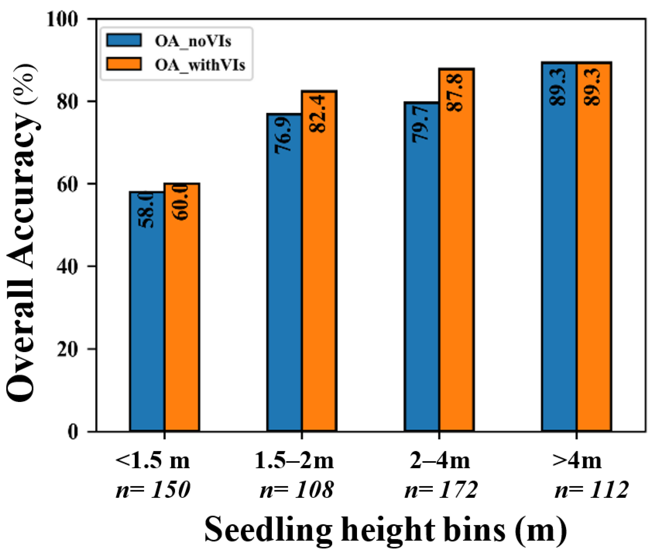
4.5. The Effects of Seedling-Tree Height and Number of C_th-Affected Pixels on the Accuracy of Species Classification in CNN and RF

This study discovered two influential factors with respect to the performance of species classification accuracy, including (1) the proportion of C_th-affected pixels inside a tensor; and (2) the seedling heights.

Based on the results obtained in this research, the classification of short trees (i.e., shorter than 1.5 m) was challenging, as was the classification of tensors with a >40%-C_th-affection rate. These two factors hampered the classification of seedlings in general and could be considered as a similar factor observed from different perspectives; i.e., most of the >40%-affected tensors represented trees shorter than 1.5 m. However, our developed method improved the classification of shorter seedlings (<1.5 m) by up to 8 pp, although it was (and still is) a challenge for the classifiers. The OA was highest at bins of 2–4 m and >4 m, which could be attributed to the fact that those tensors have a smaller number of nullified pixels. There was no improvement when trees were >4 m because there were no C_th-affected tensors, so they remained unchanged.

The not-C_th-affected tensors were generally more accurately predicted than the withC_th tensors in both classifiers and datasets of withVIs and noVIs. This is not a surprise, as they often represent taller seedlings and have higher foliage canopies, which allow for a lower effect of understory, especially as the size of the tensors used was rather small. This small tensor size was to support the smaller seedlings because their canopy was often even smaller. The selected tensor size was based on a visual experiment performed to fit most of the seedlings.

Based on the results obtained in this research, the effect of employing the C_th seemed very influential on the tensors that were affected by >40% of their pixels (with an improved OA of species classification up to 12.5 pp). This was an interesting and important finding of this research because these challenging seedlings hamper species classification in general.

4.6. Feature Importance and Model Configurations of the Classifiers

The RedEdge band of the MicaSense camera was found to be important according to the selected features by RF. The VIs in which RedEdge was used were found to be the most important features in both the noC_th and withC_th datasets of RF. The importance of RedEdge was also documented in another article [66]. Moreover, there was high inter-collinearity between the features, and it is good that this was checked.

As for the CNN and RF model configurations, it was observed that an automatic procedure in both classifiers was useful in order to obtain the most-suitable parameters for the given input data and save time. It was also learned that using only default values of RF parameters yielded 67.343% using the top-five features that were selected inside the grid; hence, using GridSearch improved the accuracy by 1 pp (from 67.3% to 68.3%), which refers to an experiment carried out on the withC_th dataset (results not shown). Including dropout in CNN was useful in order to avoid overfitting and increase the generalization of the models used in this research, which was in line with Zhang et al. [56]; they suggested that using a dropout rate of 0.5 was useful, which confirmed our values (0.6 and 0.8) achieved after hyper-tuning.

4.7. General Discussion and Future Research

The dimension of the tensors was an influential parameter with respect to species classification accuracy [37,56,67]; for example, tensor dimensions of 13 × 13 (compared to 5 × 5) and 64 × 64 (compared to 32 × 32 and 48 × 48) were found to yield more accurate tree species classification in mature forests by Zhang et al. [56] and Sun et al. [67], respectively. Similarly large tensor dimensions were suggested by Li et al. [37] for tensors ranging from 16 to 64 pixels. However, considering the GSD of multispectral data used in this research (5 cm), and the smaller size of seedlings compared to mature trees, it was not possible for us, in this study, to use such large tensor dimensions, as a large tensor could include multiple seedling canopies or large understory reflectance.

Another issue was that about 7% of the field data (the tensors) had impurity of species classes, meaning that there was at least one other tree class under the main species of the tensor; for example, the main species was pine, but it included few grass/thicket-like birches. This phenomenon is common and expectable in dense and unthinned seedling stands.

Further studies using the whole dataset with C_th-affected pixels are needed, as well as those examining different heights of C_ths and filling strategies (different kernel size and kernel types such as max kernel, inverse weighted average, etc.). Moreover, further studies could investigate another approach in which training and predicting the C_th-affected and C_th-not-affected sub-datasets are undertaken separately, after which the predictions of each sub-dataset are merged. This would require more field data, especially for the C_th-affected sub-dataset. Moreover, using hyperspectral images and better atmospheric correction might further improve results; using hyperspectral data could enable the adding of more VI-bands than were used in this study. In other words, there was only one band for R, G, B, NIR, and RedEdge, which enabled us to add at least eight VIs with them, but the existence of hyperspectral data would enable many more VIs. Furthermore, a more complex and deeper CNN structure could be used, for example, to retrain the best-trained model with a new learning rate optimizer and change the activation function. The results of one of our experiments showed an improvement in the OA of up to 1.1 pp when applying the idea, but the results were not consistent (results were not shown). Finally, the GSD of the multispectral dataset used in this study was 5 cm. This limited the tensor size to 10 × 10, and, particularly for small seedlings, a large portion was nullified. It is likely that a finer resolution would improve the results, and fast development of camera technologies already allow for the collecting of multispectral imagery with a 1 cm GSD with the flight heights used in this study.

5. Conclusions

The aim of this research was to improve the species classification accuracy of seedlings using multispectral drone imagery and a state-of-the-art CNN classifier, as well as to propose and assess several methodological improvements. Successful species classification could support the smarter planning of the required silvicultural treatments in seedling stands. The applied methodological improvement on species classification using CNN and RF classifiers enhanced the classification accuracy of seedlings in boreal seedling stands. Compared to classification accuracies of CNN and RF in noC_th datasets, the OA was improved by 2.8 and 0.4 pp, respectively. Moreover, merging the C_th-affected and not-C_th-affected tensors into a new dataset improved the accuracy of species classification in CNN (up to 2.8 pp), as did adding the vegetation indices (up to 4.3 pp). In general, the CNN had a 13.3 pp-higher species classification accuracy than RF. Most notably, the difference for pine seedlings was over 50 pp.

According to the results, seedling classification was most accurate when seedlings were taller than 1.5 m and contained fewer C_th-affected cells. Although seedlings shorter than 1.5 m and containing a higher number of C_th-affected cells were challenging for both CNN and RF, applying the methodological approaches introduced in this research improved the classification of those challenging seedlings as well. In conclusion, it seems that the methodological improvement introduced in this study could be carefully included in drone-imagery-based forest inventories of seedling stands to assist silvicultural decision-making in sustainable forest management.

References

1. Fassnacht, F.E.; Latifi, H.; Stereńczak, K.; Modzelewska, A.; Lefsky, M.; Waser, L.T.; Straub, C.; Ghosh, A. Review of Studies on Tree Species Classification from Remotely Sensed Data. Remote Sens. Environ. 2016, 186, 64–87. [Google Scholar] [CrossRef]
2. Imangholiloo, M.; Saarinen, N.; Holopainen, M.; Yu, X.; Hyyppä, J.; Vastaranta, M. Using Leaf-Off and Leaf-On Multispectral Airborne Laser Scanning Data to Characterize Seedling Stands. Remote Sens. 2020, 12, 3328. [Google Scholar] [CrossRef]
3. Tapio. Hyvän Metsänhoidon Suositukset. Recommendations for Forest Management in Finland. In Forest Development Centre Tapio; Metsäkustannus Oy: Helsinki, Finland, 2006; 100p. (In Finnish) [Google Scholar]
4. Grabska, E.; Socha, J. Evaluating the Effect of Stand Properties and Site Conditions on the Forest Reflectance from Sentinel-2 Time Series. PLoS ONE 2021, 16, e0248459. [Google Scholar] [CrossRef]
5. Eriksson, H.M.; Eklundh, L.; Kuusk, A.; Nilson, T. Impact of Understory Vegetation on Forest Canopy Reflectance and Remotely Sensed LAI Estimates. Remote Sens. Environ. 2006, 103, 408–418. [Google Scholar] [CrossRef]
6. Joyce, S.; Olsson, H. Monitoring Forest Growth Using Long Time Series of Satellite Data. Int. Arch. Photogramm. Remote Sens. Spat. Inf. Sci. ISPRS Arch. 2000, 33, 1081–1088. [Google Scholar]
7. White, J.C.; Coops, N.C.; Wulder, M.A.; Vastaranta, M.; Hilker, T.; Tompalski, P. Remote Sensing Technologies for Enhancing Forest Inventories: A Review. Can. J. Remote Sens. 2016, 42, 619–641. [Google Scholar] [CrossRef]
8. Kangas, A.; Astrup, R.; Breidenbach, J.; Fridman, J.; Gobakken, T.; Korhonen, K.T.; Maltamo, M.; Nilsson, M.; Nord-Larsen, T.; Næsset, E.; et al. Remote Sensing and Forest Inventories in Nordic Countries—Roadmap for the Future. Scand. J. For. Res. 2018, 7581, 397–412. [Google Scholar] [CrossRef]
9. Hallsby, G.; Ulvcrona, K.A.; Karlsson, A.; Elfving, B.; Sjögren, H.; Ulvcrona, T.; Bergsten, U. Effects of Intensity of Forest Regeneration Measures on Stand Development in a Nationwide Swedish Field Experiment. Forestry 2015, 88, 441–453. [Google Scholar] [CrossRef]
10. Korhonen, L.; Pippuri, I.; Packalén, P.; Heikkinen, V.; Maltamo, M.; Heikkilä, J. Detection of the Need for Seedling Stand Tending Using High-Resolution Remote Sensing Data. Silva Fenn. 2013, 47, 105823. [Google Scholar] [CrossRef]
11. Uotila, K.; Saksa, T. Effects of Early Cleaning on Young Picea Abies Stands. Scand. J. For. Res. 2014, 29, 111–119. [Google Scholar] [CrossRef]
12. Huuskonen, S.; Hynynen, J. Timing and Intensity of Precommercial Thinning and Their Effects on the First Commercial Thinning in Scots Pine Stands. Silva Fenn. 2006, 40, 645–662. [Google Scholar] [CrossRef]
13. Kuuluvainen, T.; Gauthier, S. Young and Old Forest in the Boreal: Critical Stages of Ecosystem Dynamics and Management under Global Change. For. Ecosyst. 2018, 5, 26. [Google Scholar] [CrossRef]
14. Swanson, M.E.; Franklin, J.F.; Beschta, R.L.; Crisafulli, C.M.; DellaSala, D.A.; Hutto, R.L.; Lindenmayer, D.B.; Swanson, F.J. The Forgotten Stage of Forest Succession: Early-successional Ecosystems on Forest Sites. Front. Ecol. Environ. 2011, 9, 117–125. [Google Scholar] [CrossRef]
15. Uotila, K. Optimization of Early Cleaning and Precommercial Thinning Methods in Juvenile Stand Management of Norway Spruce Stands. Ph.D Thesis, Finnish Society of Forest Science, Helsinki, Finland, 2017. [Google Scholar]
16. De Lombaerde, E.; Baeten, L.; Verheyen, K.; Perring, M.P.; Ma, S.; Landuyt, D. Understorey Removal Effects on Tree Regeneration in Temperate Forests: A Meta-Analysis. J. Appl. Ecol. 2021, 58, 9–20. [Google Scholar] [CrossRef]
17. Dumas, N.; Dupouey, J.L.; Gégout, J.C.; Boulanger, V.; Bontemps, J.D.; Morneau, F.; Dalmasso, M.; Collet, C. Identification and Spatial Extent of Understory Plant Species Requiring Vegetation Control to Ensure Tree Regeneration in French Forests. Ann. For. Sci. 2022, 79, 41. [Google Scholar] [CrossRef]
18. Kaila, S.; Kiljunen, N.; Miettinen, A.; Valkonen, S. Effect of Timing of Precommercial Thinning on the Consumption of Working Time in Picea Abies Stands in Finland. Scand. J. For. Res. 2006, 21, 496–504. [Google Scholar] [CrossRef]
19. Hynynen, J.; Niemistö, P.; Viherä-Aarnio, A.; Brunner, A.; Hein, S.; Velling, P. Silviculture of Birch (Betula Pendula Roth and Betula Pubescens Ehrh.) in Northern Europe. Forestry 2010, 83, 103–119. [Google Scholar] [CrossRef]
20. Martin, M.E.; Newman, S.D.; Aber, J.D.; Congalton, R.G. Determining Forest Species Composition Using High Spectral Resolution Remote Sensing Data. Remote Sens. Environ. 1998, 65, 249–254. [Google Scholar] [CrossRef]
21. Maxwell, A.E.; Warner, T.A.; Fang, F. Implementation of Machine-Learning Classification in Remote Sensing: An Applied Review. Int. J. Remote Sens. 2018, 39, 2784–2817. [Google Scholar] [CrossRef]
22. Raczko, E.; Zagajewski, B. Comparison of Support Vector Machine, Random Forest and Neural Network Classifiers for Tree Species Classification on Airborne Hyperspectral APEX Images. Eur. J. Remote Sens. 2017, 50, 144–154. [Google Scholar] [CrossRef]
23. Breiman, L. Random Forests. Mach. Learn. 2001, 45, 5–32. [Google Scholar] [CrossRef]
24. Pedregosa, F.; Varoquaux, G.; Gramfort, A.; Michel, V.; Thirion, B.; Grisel, O.; Blondel, M.; Prettenhofer, P.; Weiss, R.; Dubourg, V.; et al. Scikit-Learn: Machine Learning in Python. J. Mach. Learn. Res. 2011, 12, 2825–2830. [Google Scholar]
25. Ma, L.; Liu, Y.; Zhang, X.; Ye, Y.; Yin, G.; Johnson, B.A. Deep Learning in Remote Sensing Applications: A Meta-Analysis and Review. ISPRS J. Photogramm. Remote Sens. 2019, 152, 166–177. [Google Scholar] [CrossRef]
26. Litjens, G.; Kooi, T.; Bejnordi, B.E.; Setio, A.A.A.; Ciompi, F.; Ghafoorian, M.; van der Laak, J.A.W.M.; van Ginneken, B.; Sánchez, C.I. A Survey on Deep Learning in Medical Image Analysis. Med. Image Anal. 2017, 42, 60–88. [Google Scholar] [CrossRef]
27. Alzubaidi, L.; Zhang, J.; Humaidi, A.J.; Al-Dujaili, A.; Duan, Y.; Al-Shamma, O.; Santamaría, J.; Fadhel, M.A.; Al-Amidie, M.; Farhan, L. Review of Deep Learning: Concepts, CNN Architectures, Challenges, Applications, Future Directions; Springer International Publishing: Berlin/Heidelberg, Germany, 2021; Volume 8, ISBN 4053702100444. [Google Scholar]
28. Gao, Q.; Lim, S.; Jia, X. Hyperspectral Image Classification Using Convolutional Neural Networks and Multiple Feature Learning. Remote Sens. 2018, 10, 299. [Google Scholar] [CrossRef]
29. Li, Y.; Zhang, H.; Shen, Q. Spectral-Spatial Classification of Hyperspectral Imagery with 3D Convolutional Neural Network. Remote Sens. 2017, 9, 67. [Google Scholar] [CrossRef]
30. Mäyrä, J.; Keski-Saari, S.; Kivinen, S.; Tanhuanpää, T.; Hurskainen, P.; Kullberg, P.; Poikolainen, L.; Viinikka, A.; Tuominen, S.; Kumpula, T.; et al. Tree Species Classification from Airborne Hyperspectral and LiDAR Data Using 3D Convolutional Neural Networks. Remote Sens. Environ. 2021, 256, 112322. [Google Scholar] [CrossRef]
31. Natesan, S.; Armenakis, C.; Vepakomma, U. Individual Tree Species Identification Using Dense Convolutional Network (Densenet) on Multitemporal RGB Images from UAV. J. Unmanned Veh. Syst. 2020, 8, 310–333. [Google Scholar] [CrossRef]
32. Nezami, S.; Khoramshahi, E.; Nevalainen, O.; Pölönen, I.; Honkavaara, E. Tree Species Classification of Drone Hyperspectral and RGB Imagery with Deep Learning Convolutional Neural Networks. Remote Sens. 2020, 12, 1070. [Google Scholar] [CrossRef]
33. Yan, S.; Jing, L.; Wang, H. A New Individual Tree Species Recognition Method Based on a Convolutional Neural Network and High-spatial Resolution Remote Sensing Imagery. Remote Sens. 2021, 13, 479. [Google Scholar] [CrossRef]
34. Fricker, G.A.; Ventura, J.D.; Wolf, J.A.; North, M.P.; Davis, F.W.; Franklin, J. A Convolutional Neural Network Classifier Identifies Tree Species in Mixed-Conifer Forest from Hyperspectral Imagery. Remote Sens. 2019, 11, 2326. [Google Scholar] [CrossRef]
35. Pleşoianu, A.I.; Stupariu, M.S.; Şandric, I.; Pătru-Stupariu, I.; Drăguţ, L. Individual Tree-Crown Detection and Species Classification in Very High-Resolution Remote Sensing Imagery Using a Deep Learning Ensemble Model. Remote Sens. 2020, 12, 2426. [Google Scholar] [CrossRef]
36. Guo, X.; Li, H.; Jing, L.; Wang, P. Individual Tree Species Classification Based on Convolutional Neural Networks and Multitemporal High-Resolution Remote Sensing Images. Sensors 2022, 22, 3157. [Google Scholar] [CrossRef]
37. Li, H.; Hu, B.; Li, Q.; Jing, L. Cnn-Based Individual Tree Species Classification Using High-Resolution Satellite Imagery and Airborne Lidar Data. Forests 2021, 12, 1697. [Google Scholar] [CrossRef]
38. Pearse, G.D.; Tan, A.Y.S.; Watt, M.S.; Franz, M.O.; Dash, J.P. Detecting and Mapping Tree Seedlings in UAV Imagery Using Convolutional Neural Networks and Field-Verified Data. ISPRS J. Photogramm. Remote Sens. 2020, 168, 156–169. [Google Scholar] [CrossRef]
39. Hartley, R.J.L.; Leonardo, E.M.; Massam, P.; Watt, M.S.; Estarija, H.J.; Wright, L.; Melia, N.; Pearse, G.D. An Assessment of High-Density UAV Point Clouds for the Measurement of Young Forestry Trials. Remote Sens. 2020, 12, 4039. [Google Scholar] [CrossRef]
40. Chadwick, A.J.; Goodbody, T.R.H.; Coops, N.C.; Hervieux, A.; Bater, C.W.; Martens, L.A.; White, B.; Röeser, D. Automatic Delineation and Height Measurement of Regenerating Conifer Crowns under Leaf-off Conditions Using Uav Imagery. Remote Sens. 2020, 12, 4104. [Google Scholar] [CrossRef]
41. Fromm, M.; Schubert, M.; Castilla, G.; Linke, J.; McDermid, G. Automated Detection of Conifer Seedlings in Drone Imagery Using Convolutional Neural Networks. Remote Sens. 2019, 11, 2585. [Google Scholar] [CrossRef]
42. Næsset, E.; Bjerknes, K.-O. Estimating Tree Heights and Number of Stems in Young Forest Stands Using Airborne Laser Scanner Data. Remote Sens. Environ. 2001, 78, 328–340. [Google Scholar] [CrossRef]
43. Korpela, I.; Tuomola, T.; Tokola, T.; Dahlin, B. Appraisal of Seedling Stand Vegetation with Airborne Imagery and Discrete-Return LiDAR—an Exploratory Analysis. Silva Fenn. 2008, 42, 753–772. [Google Scholar] [CrossRef]
44. Økseter, R.; Bollandsås, O.M.; Gobakken, T.; Næsset, E. Modeling and Predicting Aboveground Biomass Change in Young Forest Using Multi-Temporal Airborne Laser Scanner Data. Scand. J. For. Res. 2015, 30, 458–469. [Google Scholar] [CrossRef]
45. Imangholiloo, M.; Yrttimaa, T.; Mattsson, T.; Junttila, S.; Holopainen, M.; Saarinen, N.; Savolainen, P.; Hyyppä, J.; Vastaranta, M. Adding Single Tree Features and Correcting Edge Tree Effects Enhance the Characterization of Seedling Stands with Single-Photon Airborne Laser Scanning. ISPRS J. Photogramm. Remote Sens. 2022, 191, 129–142. [Google Scholar] [CrossRef]
46. Imangholiloo, M.; Saarinen, N.; Markelin, L.; Rosnell, T.; Näsi, R.; Hakala, T.; Honkavaara, E.; Holopainen, M.; Hyyppä, J.; Vastaranta, M. Characterizing Seedling Stands Using Leaf-Off and Leaf-On Photogrammetric Point Clouds and Hyperspectral Imagery Acquired from Unmanned Aerial Vehicle. Forests 2019, 10, 415. [Google Scholar] [CrossRef]
47. Falbel, D.; Allaire, J.J.; Chollet, F. Keras Open-Source Neural-Network Library Written in Python v2.13.1. 2015. Available online: https://github.com/keras-team/keras (accessed on 31 January 2023).
48. Abadi, M.; Barham, P.; Chen, J.; Chen, Z.; Davis, A.; Dean, J.; Devin, M.; Ghemawat, S.; Irving, G.; Isard, M.; et al. Tensorflow: A System for Large-Scale Machine Learning. In Proceedings of the 12th Symposium on Operating Systems Design and ImplementationSymposium on Operating Systems Design and Implementation, Savannah, GA, USA, 2–4 November 2016; pp. 265–283. [Google Scholar]
49. Bauerle, A.; Van Onzenoodt, C.; Ropinski, T. Net2Vis-A Visual Grammar for Automatically Generating Publication-Tailored CNN Architecture Visualizations. IEEE Trans. Vis. Comput. Graph. 2021, 27, 2980–2991. [Google Scholar] [CrossRef] [PubMed]
50. Hinton, G.E.; Srivastava, N.; Krizhevsky, A.; Sutskever, I.; Salakhutdinov, R.R. Improving Neural Networks by Preventing Co-Adaptation of Feature Detectors. arXiv 2012, arXiv:1207.0580. [Google Scholar]
51. Srivastava, N.; Hinton, G.; Krizhevsky, A.; Sutskever, I.; Salakhutdinov, R. Dropout: A Simple Way to Prevent Neural Networks from Overfitting. J. Mach. Learn. Res. 2014, 15, 1929–1958. [Google Scholar]
52. Varshney, M.; Singh, P. Optimizing Nonlinear Activation Function for Convolutional Neural Networks. Signal, Image Video Process. 2021, 15, 1323–1330. [Google Scholar] [CrossRef]
53. CSC—IT Center for Science Finland. Supercomputer Puhti Is Now Available for Researchers—Supercomputer Puhti Is Now Available for Researchers. CSC Company Site. 2022. Available online: https://www.csc.fi/En/-/Supertietokone-Puhti-on-Avattu-Tutkijoiden-Kayttoon (accessed on 31 January 2023).
54. Prasad, M.P.S.; Senthilrajan, A. A Novel CNN-KNN Based Hybrid Method for Plant Classification. J. Algebr. Stat. 2022, 13, 498–502. [Google Scholar]
55. Chen, C.; Jing, L.; Li, H.; Tang, Y. A New Individual Tree Species Classification Method Based on the Resu-Net Model. Forests 2021, 12, 1202. [Google Scholar] [CrossRef]
56. Zhang, B.; Zhao, L.; Zhang, X. Three-Dimensional Convolutional Neural Network Model for Tree Species Classification Using Airborne Hyperspectral Images. Remote Sens. Environ. 2020, 247, 111938. [Google Scholar] [CrossRef]
57. Ao, L.; Feng, K.; Sheng, K.; Zhao, H.; He, X.; Chen, Z. TPENAS: A Two-Phase Evolutionary Neural Architecture Search for Remote Sensing Image Classification. Remote Sens. 2023, 15, 2212. [Google Scholar] [CrossRef]
58. Martins, G.B.; La Rosa, L.E.C.; Happ, P.N.; Filho, L.C.T.C.; Santos, C.J.F.; Feitosa, R.Q.; Ferreira, M.P. Deep Learning-Based Tree Species Mapping in a Highly Diverse Tropical Urban Setting. Urban For. Urban Green. 2021, 64, 127241. [Google Scholar] [CrossRef]
59. Anderson, C.J.; Heins, D.; Pelletier, K.C.; Knight, J.F. Improving Machine Learning Classifications of Phragmites Australis Using Object-Based Image Analysis. Remote Sens. 2023, 15, 989. [Google Scholar] [CrossRef]
60. Xi, Y.; Ren, C.; Wang, Z.; Wei, S.; Bai, J.; Zhang, B.; Xiang, H.; Chen, L. Mapping Tree Species Composition Using OHS-1 Hyperspectral Data and Deep Learning Algorithms in Changbai Mountains, Northeast China. Forests 2019, 10, 818. [Google Scholar] [CrossRef]
61. Hartling, S.; Sagan, V.; Sidike, P.; Maimaitijiang, M.; Carron, J. Urban Tree Species Classification Using a Worldview-2/3 and LiDAR Data Fusion Approach and Deep Learning. Sensors 2019, 19, 1284. [Google Scholar] [CrossRef]
62. Ye, N.; Morgenroth, J.; Xu, C.; Chen, N. Indigenous Forest Classification in New Zealand—A Comparison of Classifiers and Sensors. Int. J. Appl. Earth Obs. Geoinf. 2021, 102, 102395. [Google Scholar] [CrossRef]
63. Adagbasa, E.G.; Adelabu, S.A.; Okello, T.W. Application of Deep Learning with Stratified K-Fold for Vegetation Species Discrimation in a Protected Mountainous Region Using Sentinel-2 Image. Geocarto Int. 2022, 37, 142–162. [Google Scholar] [CrossRef]
64. Trier, Ø.D.; Salberg, A.B.; Kermit, M.; Rudjord, Ø.; Gobakken, T.; Næsset, E.; Aarsten, D. Tree Species Classification in Norway from Airborne Hyperspectral and Airborne Laser Scanning Data. Eur. J. Remote Sens. 2018, 51, 336–351. [Google Scholar] [CrossRef]
65. Yaloveha, V.; Hlavcheva, D.; Podorozhniak, A. Spectral Indexes Evaluation for Satellite Images Classification Using CNN. J. Inf. Organ. Sci. 2021, 45, 435–449. [Google Scholar] [CrossRef]
66. Zhu, Y.; Liu, K.; Liu, L.; Myint, S.W.; Wang, S.; Liu, H.; He, Z. Exploring the Potential of World View-2 Red-Edge Band-Based Vegetation Indices for Estimation of Mangrove Leaf Area Index with Machine Learning Algorithms. Remote Sens. 2017, 9, 1060. [Google Scholar] [CrossRef]
67. Sun, Y.; Xin, Q.; Huang, J.; Huang, B.; Zhang, H. Characterizing Tree Species of a Tropical Wetland in Southern China at the Individual Tree Level Based on Convolutional Neural Network. IEEE J. Sel. Top. Appl. Earth Obs. Remote Sens. 2019, 12, 4415–4425. [Google Scholar] [CrossRef]
Figure 1. A map of the study area in southern Finland (A) showing the five flight zones with drone-based red, green, blue (RGB) orthomosaics (B), together with a drone-based multispectral orthomosaic in a flight zone (C) and zooming into a single forest stand (D) and forest plot (10 × 10 m, (E)), showing tensors of field-measured trees (10 × 10 pixels). Numbers 1, 2, 3, and 4 in (E) show species classes of pine, spruce, birch, and other species, respectively. The topographical map in (B) is from the National Land Survey of Finland (NLS).
Remotesensing 15 05233 g001
Figure 2. Visualizing the effect of applying the canopy threshold (Cth)-based image pre-processing method introduced in this research on two sample pine trees with height 1.4 m (upper row) and 1.3 m (lower row). The pixel size of the RGB image is 1.4 cm, but CHM and multispectral images are 5 cm. The multispectral images (noCth and withCth) visualized colored infrared bands (bands 5, 3, 2). The CHM is pseudo-colored by height (legend in each separately). The white pixels in CHM denote nullified (Cth-affected) pixels after image pre-processing due to a height of ≤0.4. The + symbol in the middle of the images shows the location of a field-measured treetop.
Remotesensing 15 05233 g002
Figure 3. The model architecture used in this research.
Remotesensing 15 05233 g003
Figure 4. A schematic graph of the methodological principles behind introducing canopy threshold (Cth)-based image pre-processing and combining two subsets of the test dataset based on whether or not it was affected by Cth processing.
Remotesensing 15 05233 g004
Figure 5. Overall accuracy within the canopy threshold (Cth)-affected (n = 161, 33.4%) and not-affected (n = 361, 66.6%) subsets of the test set (n = 542) in RF, CNN noVIs (without vegetation indices, five bands), and CNN withVIs (after fusing 8 VIs to tensors pixels, 13 bands) in the original (noCth) and Cth-applied (withCth) datasets.
Remotesensing 15 05233 g005
Figure 6. Plotting overall accuracy of species classification within different Cth-affection rates (%); in fact, 0 refers to not-Cth-affected, and the rest of bars are barplots of Cth-affection (%, also real numbers too because it was 10 × 10). The italic number “n=” shows the number of test datasets included in that bin. noVIs: without fusing vegetation indices (VIs) to CNN; withVIs: with fusing VIs.
Remotesensing 15 05233 g006
Figure 7. Plotting overall accuracy of species classification considering seedlings height (meter). The italic number “n=” indicates the number of tensors included in that height bin. noVIs: without fusing vegetation indices (VIs) to CNN; withVIs: with fusing VIs.
Remotesensing 15 05233 g007
Figure 8. The summary of species classification accuracies in the normalized confusion matrix together with overall accuracy and kappa values. RF: random forest classifier; CNN: convolutional neural network; Vis: vegetation indices. Values inside each cell show the recall values of the cell – proportion of correctly classified class over the total observations of the class.
Remotesensing 15 05233 g008
Figure 9. Plotting overall accuracy of species classification within different Cth-affection rates (%); in fact, 0 refers to not-Cth-affected, and the rest of bars are barplots of Cth-affection (%). The italic number “n=” shows the number of tensors included in that bin. noVIs: without fusing vegetation indices (VIs) to CNN; withVIs: with fusing VIs.
Remotesensing 15 05233 g009
Figure 10. Visualizing overall accuracy of species classification regarding seedlings height (meter). The italic number “n=” shows the number of tensors that the height bin included. noVIs: without fusing vegetation indices (VIs) to CNN; withVIs: with fusing VIs.
Remotesensing 15 05233 g010
Figure 11. The summary of species classification accuracies in the normalized confusion matrix including overall accuracy and kappa values. RF: random forest classifier; CNN: convolutional neural network; VIs: vegetation indices. Values inside each cell are the recall of the cell.
Remotesensing 15 05233 g011
Figure 12. Selected five most important and not-intercorrelated (<0.8) features for RF in the noCth and withCth datasets. Correlation matrix (upper-right) and scatter plot with fitting regression (lower-left) and histogram (diagonal 1:1 line).
Remotesensing 15 05233 g012