
Data-Driven Landslide Spatial Prediction and Deformation Monitoring: A Case Study of Shiyan City, China


Abstract
:1. Introduction
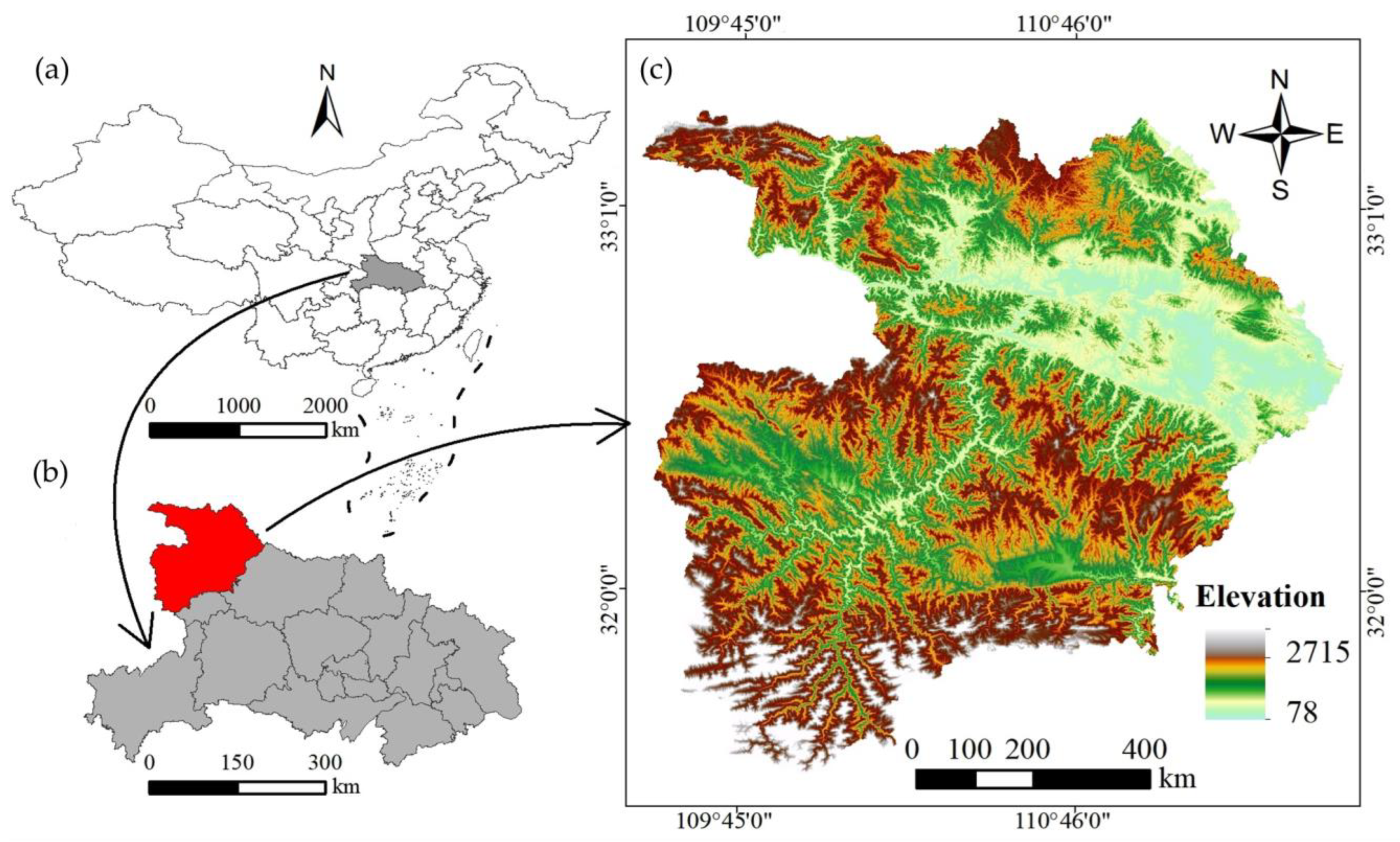
2. Study Area
3. Methodologies
3.1. Landslide Susceptibility Mapping
3.1.1. Statistical Analysis Methods
- (a)
- Information quantity (IQ)
- (b)
- Frequency ratio (FR)
- (c)
- Logistic regression (LR)
3.1.2. Machine Learning Methods
- (a)
- Artificial neural network (ANN)
- (b)
- Random forest (RF)
- (c)
- Support vector machine (SVM)
- (d)
- Convolutional neural network (CNN)
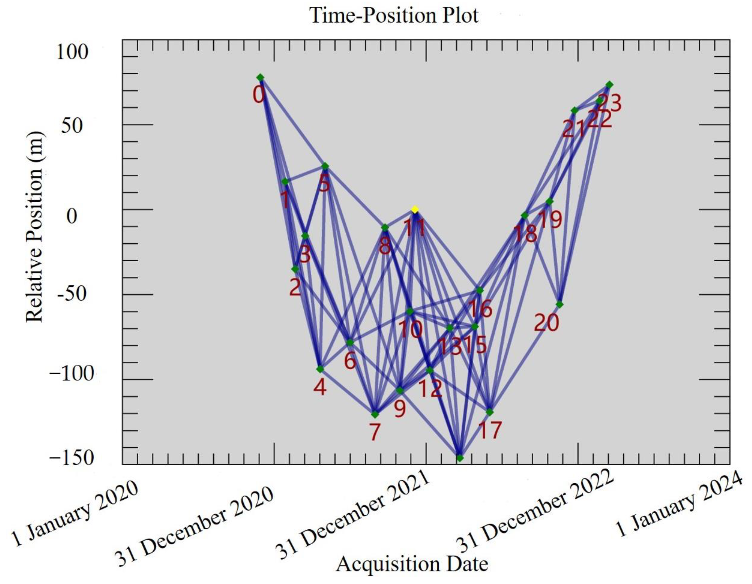
3.1.3. Time-Series InSAR Process
3.2. Modelling Prediction and Performance
3.3. Methodological Flowchart
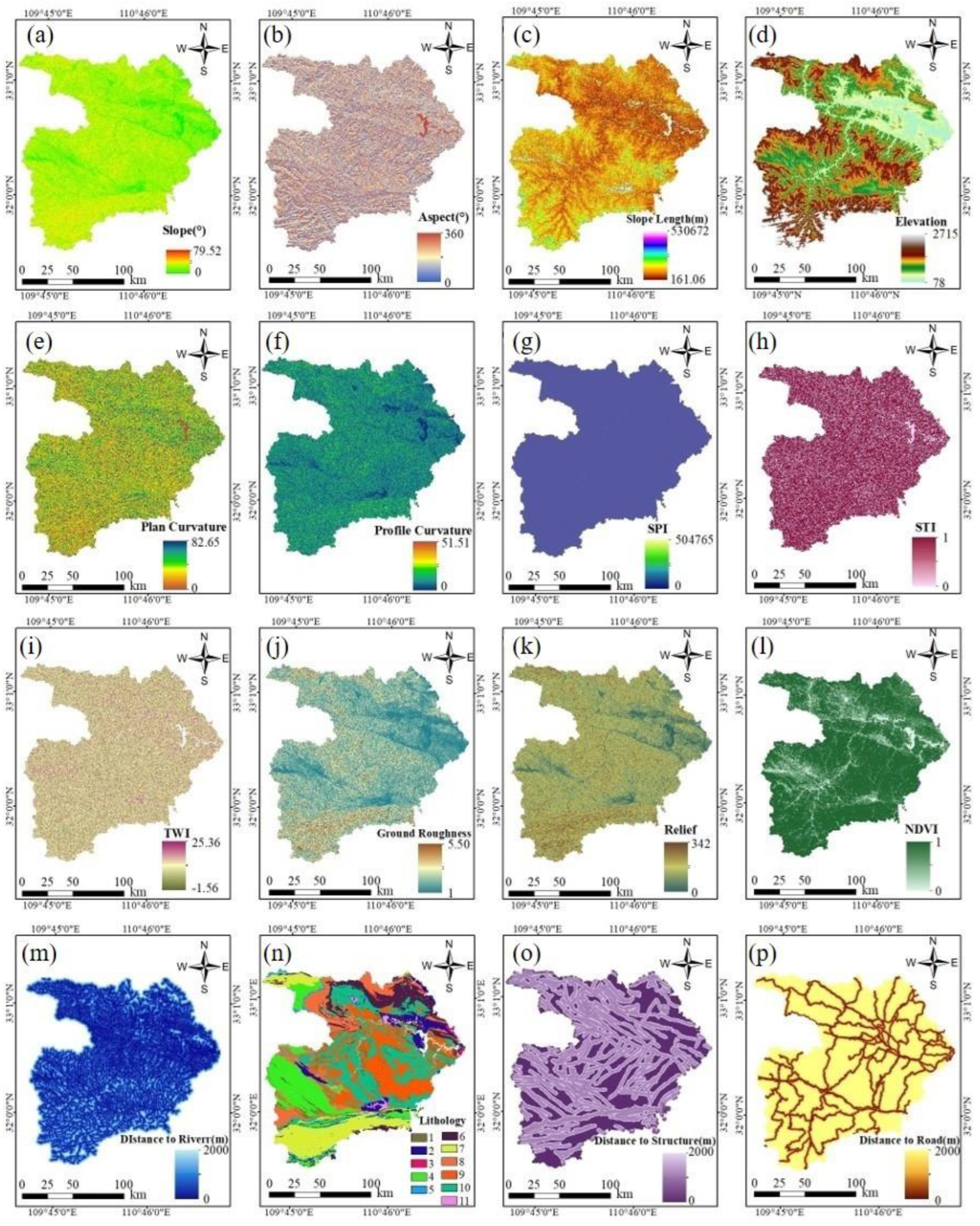
4. Selection of Causal Factors
4.1. Landslide Inventory Map
4.2. Contribution Analysis of Influencing Factors
5. Landslide Susceptibility Modelling
5.1. Parameter Determination of Machine Learning
5.2. Modelling Process of Machine Learning
- (i)
- The training dataset was imported into the software, where the influence factor values for each unit were derived using the GIS and subsequently fed into the constructed SVM model. The probabilities of landslide occurrences within these units were computed, with all values standardized on a dimensionless scale spanning from 0 to 1.
- (ii)
- The factor values of all identified landslide points, combined with a comparable number of non-landslide points and their respective states (zero denoting non-landslide and one indicating landslide), were amalgamated into a consolidated matrix. This matrix was utilized as input for the MATLAB 2021 to assess the contribution of each factor. Following this analysis, the penalty and RBF kernel parameters were determined as the definitive configuration, documented in Table 6.
- (iii)
- The probability matrix, obtained from step (ii), indicating the likelihood of landslide occurrences, was imported into the SPSS 24.0. The K-means clustering algorithm was employed on the dataset to identify and define the five centroids. Data points near each centroid were subsequently reclassified into their respective groups, with each centroid representing the central focal point of its group. The average value between two adjacent centroids was implemented as the threshold for segregating distinct susceptibility bands, as it effectively discriminated between datasets exhibiting diverse properties. Accordingly, a comprehensive landslide susceptibility map was delineated, effectively partitioning the study area into four discrete susceptibility zones: low, medium, high, and extremely high.
- (iv)
- The model’s effectiveness, as assessed by diverse statistical indicators elucidated in Section 3.2, was substantiated by scrutinizing the spatial distribution of both landslide inventory points and randomly sampled points. This meticulous analysis facilitated a comprehensive assessment of performance relative to alternative methodologies.
6. Discussion and Comparison Analysis
6.1. Factor Effects on Landslides
6.2. Landslide Susceptibility Mapping
6.3. Accuracy Assessment and Comparison
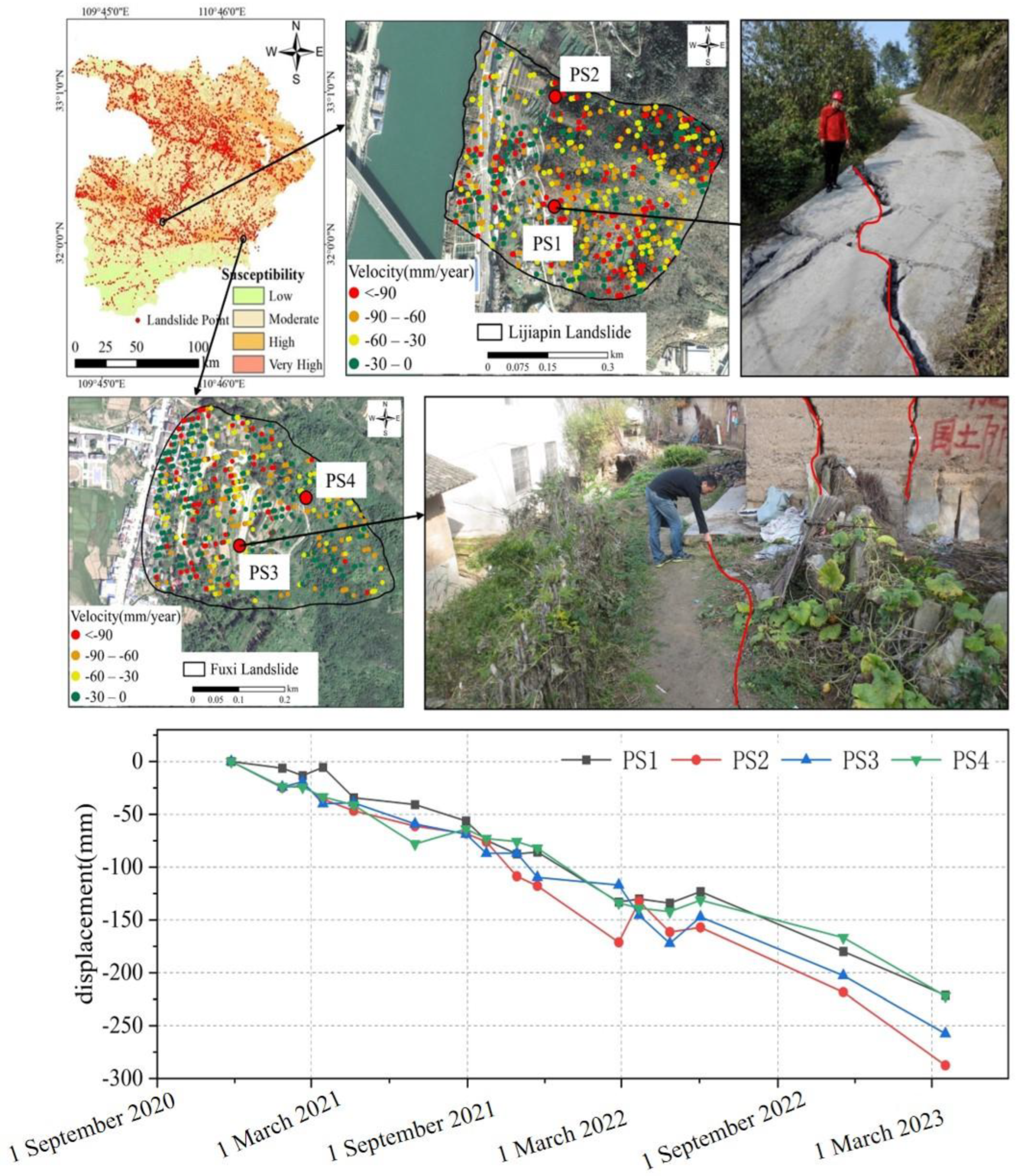
6.4. Typical Landslide Deformation Analysis
7. Conclusions
- (1)
- By remote sensing images and field investigations, sixteen landslide influencing factors, including topographical, hydrological environment, basic geological, and human engineering activity factors, were considered to construct the landslide inventory map. Additionally, different sensitivity analysis methods, such as Pearson correlation analysis, multicollinearity analysis, information gain ratio, and GeoDetector, were used to determine the importance of these factors to landslides. The results identified STI, plan curvature, TRI, and slope length as factors to be excluded when drawing LSMs.
- (2)
- The LSM results by different methods demonstrated that the material basis and internal geological conditions of landslide development were mainly affected by internal factors such as slope structure (along slope), fault distance (<200 m), formation lithology, and slope degree (6°, 20°). For external factors, landslide occurrence was primarily affected by water distance (<200 m) and road distance (<50 m). Moreover, the comparison of frequency values showed that the CNN method had the best performance, supported by the highest frequency at very high and highly sensitive levels and the lowest frequency at low sensitivity levels among the different data-driven methods.
- (3)
- By comparing the model performance, it was determined that the training and prediction accuracy of machine learning methods was higher than that of the statistical methods. For example, the AUC values for the IQ, FR, LR, BP-ANN, RBF-ANN, RF, SVM, and CNN methods were 0.810, 0.854, 0.828, 0.895, 0.916, 0.932, 0.948, and 0.957, respectively. For the F1-measure of test datasets for different machine learning methods, the largest value was for CNN (0.987), followed by SVM (0.940), RF (0.953), BP-ANN (0.953), and RBF-ANN (0.926). Given other statistical indicators, such as SPE, ACC, and Jaccard, although the performance order varied according to indicators, overall, the CNN method was the best, and the BP-ANN and RBF-ANN methods were the worst. This indicates that CNN has better nonlinear predictive ability than the traditional statistical model. When the nonlinear relationship between landslides and their influencing factors is more complex, the advantage of CNN will be more apparent.
Author Contributions
Funding
Data Availability Statement
Acknowledgments
Conflicts of Interest
References
- Chen, W.; Zhao, X.; Tsangaratos, P.; Shahabi, H.; Ilia, I.; Xue, W.; Wang, X.; Ahmad, B.B. Evaluating the usage of tree-based ensemble methods in groundwater spring potential mapping. J. Hydrol. 2020, 583, 124602. [Google Scholar] [CrossRef]
- Chikalamo, E.E.; Mavrouli, O.C.; Ettema, J.; van Westen, C.J.; Muntohar, A.S.; Mustofa, A. Satellite-derived rainfall thresholds for landslide early warning in Bogowonto Catchment, Central Java, Indonesia. Int. J. Appl. Earth Obs. Geoinf. 2020, 89, 102093. [Google Scholar] [CrossRef]
- Huang, F.; Cao, Z.; Guo, J.; Jiang, S.-H.; Li, S.; Guo, Z. Comparisons of heuristic, general statistical and machine learning models for landslide susceptibility prediction and mapping. Catena 2020, 191, 104580. [Google Scholar] [CrossRef]
- Khosravi, K.; Shahabi, H.; Pham, B.T.; Adamowski, J.; Shirzadi, A.; Pradhan, B.; Dou, J.; Ly, H.-B.; Gróf, G.; Ho, H.L.; et al. A comparative assessment of flood susceptibility modeling using Multi-Criteria Decision-Making Analysis and Machine Learning Methods. J. Hydrol. 2019, 573, 311–323. [Google Scholar] [CrossRef]
- Tien Bui, D.; Hoang, N.D.; Martinez-Alvarez, F.; Ngo, P.T.; Hoa, P.V.; Pham, T.D.; Samui, P.; Costache, R. A novel deep learning neural network approach for predicting flash flood susceptibility: A case study at a high frequency tropical storm area. Sci. Total Environ. 2020, 701, 134413. [Google Scholar] [CrossRef]
- Balogun, A.-L.; Rezaie, F.; Pham, Q.B.; Gigović, L.; Drobnjak, S.; Aina, Y.A.; Panahi, M.; Yekeen, S.T.; Lee, S. Spatial prediction of landslide susceptibility in western Serbia using hybrid support vector regression (SVR) with GWO, BAT and COA algorithms. Geosci. Front. 2021, 12, 101104. [Google Scholar] [CrossRef]
- Cai, H.; Chen, T.; Niu, R.; Plaza, A. Landslide Detection Using Densely Connected Convolutional Networks and Environmental Conditions. IEEE J. Sel. Top. Appl. Earth Obs. Remote Sens. 2021, 14, 5235–5247. [Google Scholar] [CrossRef]
- Crawford, M.H.; Crowley, K.; Potter, S.H.; Saunders, W.S.A.; Johnston, D.M. Risk modelling as a tool to support natural hazard risk management in New Zealand local government. Int. J. Disaster Risk Reduct. 2018, 28, 610–619. [Google Scholar] [CrossRef]
- Sheng, Y.; Li, Y.; Xu, G.; Li, Z. Threshold assessment of rainfall-induced landslides in Sangzhi County: Statistical analysis and physical model. Bull. Eng. Geol. Environ. 2022, 81, 388. [Google Scholar] [CrossRef]
- Youssef, A.M.; Pourghasemi, H.R. Landslide susceptibility mapping using machine learning algorithms and comparison of their performance at Abha Basin, Asir Region, Saudi Arabia. Geosci. Front. 2021, 12, 639–655. [Google Scholar] [CrossRef]
- Chang, Z.; Du, Z.; Zhang, F.; Huang, F.; Chen, J.; Li, W.; Guo, Z. Landslide Susceptibility Prediction Based on Remote Sensing Images and GIS: Comparisons of Supervised and Unsupervised Machine Learning Models. Remote Sens. 2020, 12, 502. [Google Scholar] [CrossRef]
- Hamedi, H.; Alesheikh, A.A.; Panahi, M.; Lee, S. Landslide susceptibility mapping using deep learning models in Ardabil province, Iran. Stoch. Environ. Res. Risk Assess. 2022, 36, 4287–4310. [Google Scholar] [CrossRef]
- Aditian, A.; Kubota, T.; Shinohara, Y. Comparison of GIS-based landslide susceptibility models using frequency ratio, logistic regression, and artificial neural network in a tertiary region of Ambon, Indonesia. Geomorphology 2018, 318, 101–111. [Google Scholar] [CrossRef]
- Kim, J.; Lee, K.; Jeong, S.; Kim, G. GIS-based prediction method of landslide susceptibility using a rainfall infiltration-groundwater flow model. Eng. Geol. 2014, 182, 63–78. [Google Scholar] [CrossRef]
- Liu, J.-J.; Liu, J.-C. Integrating deep learning and logging data analytics for lithofacies classification and 3D modeling of tight sandstone reservoirs. Geosci. Front. 2022, 13, 101311. [Google Scholar] [CrossRef]
- Pudasaini, S.P.; Mergili, M. A Multi-Phase Mass Flow Model. J. Geophys. Res. Earth Surf. 2019, 124, 2920–2942. [Google Scholar] [CrossRef]
- Heller, V.; Ruffini, G. A critical review about generic subaerial landslide-tsunami experiments and options for a needed step change. Earth-Sci. Rev. 2023, 242, 104459. [Google Scholar]
- Wang, H.; Jiang, Z.; Xu, W.; Wang, R.; Xie, W. Physical model test on deformation and failure mechanism of deposit landslide under gradient rainfall. Bull. Eng. Geol. Environ. 2022, 81, 02913. [Google Scholar] [CrossRef]
- Miao, F.; Wu, Y.; Li, L.; Tang, H.; Li, Y. Centrifuge model test on the retrogressive landslide subjected to reservoir water level fluctuation. Eng. Geol. 2018, 245, 169–179. [Google Scholar] [CrossRef]
- Miao, F.; Wu, Y.; Török, Á.; Li, L.; Xue, Y. Centrifugal model test on a riverine landslide in the Three Gorges Reservoir induced by rainfall and water level fluctuation. Geosci. Front. 2022, 13, 101378. [Google Scholar] [CrossRef]
- Sulpizio, R.; Castioni, D.; Rodriguez-Sedano, L.A.; Sarocchi, D.; Lucchi, F. The influence of slope-angle ratio on the dynamics of granular flows: Insights from laboratory experiments. Bull. Volcanol. 2016, 78, 77. [Google Scholar] [CrossRef]
- McDougall, S. 2014 Canadian Geotechnical Colloquium: Landslide runout analysis—Current practice and challenges. Can. Geotech. J. 2017, 54, 605–620. [Google Scholar] [CrossRef]
- Li, W.C.; Li, H.J.; Dai, F.C.; Lee, L.M. Discrete element modeling of a rainfall-induced flowslide. Eng. Geol. 2012, 149–150, 22–34. [Google Scholar] [CrossRef]
- Li, Y.; Chen, J.; Yan, J.; Zhou, F.; Wang, Q.; Li, Z.; Zhang, Y. Formation and evolution of a giant old deposit in the First Bend of the Yangtze River on the southeastern margin of the Qinghai-Tibet Plateau. Catena 2022, 213, 106138. [Google Scholar] [CrossRef]
- Zhu, Y.; Liu, C.; Liu, H.; Kou, Y.-D.; Shi, B. A multi-field and fluid–solid coupling method for porous media based on DEM-PNM. Comput. Geotech. 2023, 154, 105118. [Google Scholar] [CrossRef]
- Chen, W.; Li, Y.; Xue, W.; Shahabi, H.; Li, S.; Hong, H.; Wang, X.; Bian, H.; Zhang, S.; Pradhan, B.; et al. Modeling flood susceptibility using data-driven approaches of naive Bayes tree, alternating decision tree, and random forest methods. Sci. Total Environ. 2020, 701, 134979. [Google Scholar] [CrossRef]
- Pham, B.T.; Luu, C.; Phong, T.V.; Trinh, P.T.; Shirzadi, A.; Renoud, S.; Asadi, S.; Le, H.V.; von Meding, J.; Clague, J.J. Can deep learning algorithms outperform benchmark machine learning algorithms in flood susceptibility modeling? J. Hydrol. 2021, 592, 125615. [Google Scholar] [CrossRef]
- Reichenbach, P.; Rossi, M.; Malamud, B.D.; Mihir, M.; Guzzetti, F. A review of statistically-based landslide susceptibility models. Earth-Sci. Rev. 2018, 180, 60–91. [Google Scholar] [CrossRef]
- Ali, S.A.; Parvin, F.; Vojteková, J.; Costache, R.; Linh, N.T.T.; Pham, Q.B.; Vojtek, M.; Gigović, L.; Ahmad, A.; Ghorbani, M.A. GIS-based landslide susceptibility modeling: A comparison between fuzzy multi-criteria and machine learning algorithms. Geosci. Front. 2021, 12, 857–876. [Google Scholar] [CrossRef]
- Galanti, Y.; Barsanti, M.; Cevasco, A.; D’Amato Avanzi, G.; Giannecchini, R. Comparison of statistical methods and multi-time validation for the determination of the shallow landslide rainfall thresholds. Landslides 2018, 15, 937–952. [Google Scholar] [CrossRef]
- Pourghasemi, H.R.; Gayen, A.; Edalat, M.; Zarafshar, M.; Tiefenbacher, J.P. Is multi-hazard mapping effective in assessing natural hazards and integrated watershed management? Geosci. Front. 2020, 11, 1203–1217. [Google Scholar] [CrossRef]
- Panahi, M.; Gayen, A.; Pourghasemi, H.R.; Rezaie, F.; Lee, S. Spatial prediction of landslide susceptibility using hybrid support vector regression (SVR) and the adaptive neuro-fuzzy inference system (ANFIS) with various metaheuristic algorithms. Sci. Total Environ. 2020, 741, 139937. [Google Scholar] [CrossRef] [PubMed]
- Regmi, A.D.; Devkota, K.C.; Yoshida, K.; Pradhan, B.; Pourghasemi, H.R.; Kumamoto, T.; Akgun, A. Application of frequency ratio, statistical index, and weights-of-evidence models and their comparison in landslide susceptibility mapping in Central Nepal Himalaya. Arab. J. Geosci. 2013, 7, 725–742. [Google Scholar] [CrossRef]
- Schlögel, R.; Marchesini, I.; Alvioli, M.; Reichenbach, P.; Rossi, M.; Malet, J.P. Optimizing landslide susceptibility zonation: Effects of DEM spatial resolution and slope unit delineation on logistic regression models. Geomorphology 2018, 301, 10–20. [Google Scholar] [CrossRef]
- Razavizadeh, S.; Solaimani, K.; Massironi, M.; Kavian, A. Mapping landslide susceptibility with frequency ratio, statistical index, and weights of evidence models: A case study in northern Iran. Environ. Earth Sci. 2017, 76, 499. [Google Scholar] [CrossRef]
- Zhu, A.X.; Miao, Y.; Liu, J.; Bai, S.; Zeng, C.; Ma, T.; Hong, H. A similarity-based approach to sampling absence data for landslide susceptibility mapping using data-driven methods. Catena 2019, 183, 104188. [Google Scholar] [CrossRef]
- Akgun, A.; Sezer, E.A.; Nefeslioglu, H.A.; Gokceoglu, C.; Pradhan, B. An easy-to-use MATLAB program (MamLand) for the assessment of landslide susceptibility using a Mamdani fuzzy algorithm. Comput. Geosci. 2012, 38, 23–34. [Google Scholar] [CrossRef]
- Ozer, B.C.; Mutlu, B.; Nefeslioglu, H.A.; Sezer, E.A.; Rouai, M.; Dekayir, A.; Gokceoglu, C. On the use of hierarchical fuzzy inference systems (HFIS) in expert-based landslide susceptibility mapping: The central part of the Rif Mountains (Morocco). Bull. Eng. Geol. Environ. 2019, 79, 551–568. [Google Scholar] [CrossRef]
- Mandal, K.; Saha, S.; Mandal, S. Applying deep learning and benchmark machine learning algorithms for landslide susceptibility modelling in Rorachu river basin of Sikkim Himalaya, India. Geosci. Front. 2021, 12, 101203. [Google Scholar] [CrossRef]
- Shafizadeh-Moghadam, H.; Valavi, R.; Shahabi, H.; Chapi, K.; Shirzadi, A. Novel forecasting approaches using combination of machine learning and statistical models for flood susceptibility mapping. J. Environ. Manag. 2018, 217, 1–11. [Google Scholar] [CrossRef]
- Zhao, G.; Pang, B.; Xu, Z.; Yue, J.; Tu, T. Mapping flood susceptibility in mountainous areas on a national scale in China. Sci. Total. Environ. 2018, 615, 1133–1142. [Google Scholar] [CrossRef]
- Li, W.; Fang, Z.; Wang, Y. Stacking ensemble of deep learning methods for landslide susceptibility mapping in the Three Gorges Reservoir area, China. Stoch. Environ. Res. Risk Assess. 2021, 36, 2207–2228. [Google Scholar] [CrossRef]
- Bragagnolo, L.; Silva, R.V.d.; Grzybowski, J.M.V. Artificial neural network ensembles applied to the mapping of landslide susceptibility. Catena 2020, 184, 104240. [Google Scholar] [CrossRef]
- Can, A.; Dagdelenler, G.; Ercanoglu, M.; Sonmez, H. Landslide susceptibility mapping at Ovacık-Karabük (Turkey) using different artificial neural network models: Comparison of training algorithms. Bull. Eng. Geol. Environ. 2017, 78, 89–102. [Google Scholar] [CrossRef]
- Sameen, M.I.; Pradhan, B.; Bui, D.T.; Alamri, A.M. Systematic sample subdividing strategy for training landslide susceptibility models. Catena 2020, 187, 104358. [Google Scholar] [CrossRef]
- Oh, H.-J.; Kadavi, P.R.; Lee, C.-W.; Lee, S. Evaluation of landslide susceptibility mapping by evidential belief function, logistic regression and support vector machine models. Geomat. Nat. Hazards Risk 2018, 9, 1053–1070. [Google Scholar] [CrossRef]
- Saha, S.; Saha, A.; Hembram, T.K.; Mandal, K.; Sarkar, R.; Bhardwaj, D. Prediction of spatial landslide susceptibility applying the novel ensembles of CNN, GLM and random forest in the Indian Himalayan region. Stoch. Environ. Res. Risk Assess. 2022, 36, 3597–3616. [Google Scholar] [CrossRef]
- Sun, D.; Shi, S.; Wen, H.; Xu, J.; Zhou, X.; Wu, J. A hybrid optimization method of factor screening predicated on GeoDetector and Random Forest for Landslide Susceptibility Mapping. Geomorphology 2021, 379, 107623. [Google Scholar] [CrossRef]
- Huang, F.; Zhang, J.; Zhou, C.; Wang, Y.; Huang, J.; Zhu, L. A deep learning algorithm using a fully connected sparse autoencoder neural network for landslide susceptibility prediction. Landslides 2019, 17, 217–229. [Google Scholar] [CrossRef]
- Wang, Y.; Fang, Z.; Wang, M.; Peng, L.; Hong, H. Comparative study of landslide susceptibility mapping with different recurrent neural networks. Comput. Geosci. 2020, 138, 104445. [Google Scholar] [CrossRef]
- Sameen, M.I.; Pradhan, B.; Lee, S. Application of convolutional neural networks featuring Bayesian optimization for landslide susceptibility assessment. Catena 2020, 186, 104249. [Google Scholar] [CrossRef]
- Achour, Y.; Pourghasemi, H.R. How do machine learning techniques help in increasing accuracy of landslide susceptibility maps? Geosci. Front. 2020, 11, 871–883. [Google Scholar] [CrossRef]
- Ghorbanzadeh, O.; Rostamzadeh, H.; Blaschke, T.; Gholaminia, K.; Aryal, J. A new GIS-based data mining technique using an adaptive neuro-fuzzy inference system (ANFIS) and k-fold cross-validation approach for land subsidence susceptibility mapping. Nat. Hazards 2018, 94, 497–517. [Google Scholar] [CrossRef]
- Ullah, K.; Wang, Y.; Fang, Z.; Wang, L.; Rahman, M. Multi-hazard susceptibility mapping based on Convolutional Neural Networks. Geosci. Front. 2022, 13, 101425. [Google Scholar] [CrossRef]
- Ferretti, A.; Fumagalli, A.; Novali, F.; Prati, C.; Rocca, F.; Rucci, A. A New Algorithm for Processing Interferometric Data-Stacks: SqueeSAR. IEEE Trans. Geosci. Remote Sens. 2011, 49, 3460–3470. [Google Scholar] [CrossRef]
- Berardino, P.; Fornaro, G.; Lanari, R.; Sansosti, E. A new algorithm for surface deformation monitoring based on small baseline differential SAR interferograms. IEEE Trans. Geosci. Remote Sens. 2002, 40, 2375–2383. [Google Scholar] [CrossRef]
- Bekaert, D.P.S.; Handwerger, A.L.; Agram, P.; Kirschbaum, D.B. InSAR-based detection method for mapping and monitoring slow-moving landslides in remote regions with steep and mountainous terrain: An application to Nepal. Remote Sens. Environ. 2020, 249, 111983. [Google Scholar] [CrossRef]
- Handwerger, A.L.; Booth, A.M.; Huang, M.H.; Fielding, E.J. Inferring the Subsurface Geometry and Strength of Slow-Moving Landslides Using 3-D Velocity Measurements From the NASA/JPL UAVSAR. J. Geophys. Res. Earth Surf. 2021, 126, e2020JF005898. [Google Scholar] [CrossRef]
- Wang, W.; Motagh, M.; Mirzaee, S.; Li, T.; Zhou, C.; Tang, H.; Roessner, S. The 21 July 2020 Shaziba landslide in China: Results from multi-source satellite remote sensing. Remote Sens. Environ. 2023, 295, 113669. [Google Scholar] [CrossRef]
- Wasowski, J.; Pisano, L. Long-term InSAR, borehole inclinometer, and rainfall records provide insight into the mechanism and activity patterns of an extremely slow urbanized landslide. Landslides 2019, 17, 445–457. [Google Scholar] [CrossRef]
- Zhou, C.; Cao, Y.; Hu, X.; Yin, K.; Wang, Y.; Catani, F. Enhanced dynamic landslide hazard mapping using MT-InSAR method in the Three Gorges Reservoir Area. Landslides 2022, 19, 1585–1597. [Google Scholar] [CrossRef]
- Zhou, C.; Cao, Y.; Yin, K.; Intrieri, E.; Catani, F.; Wu, L. Characteristic comparison of seepage-driven and buoyancy-driven landslides in Three Gorges Reservoir area, China. Eng. Geol. 2022, 301, 106590. [Google Scholar] [CrossRef]
- Ng, C.W.W.; Yang, B.; Liu, Z.Q.; Kwan, J.S.H.; Chen, L. Spatiotemporal modelling of rainfall-induced landslides using machine learning. Landslides 2021, 18, 2499–2514. [Google Scholar] [CrossRef]
- Shahabi, H.; Hashim, M.; Ahmad, B.B. Remote sensing and GIS-based landslide susceptibility mapping using frequency ratio, logistic regression, and fuzzy logic methods at the central Zab basin, Iran. Environ. Earth Sci. 2015, 73, 8647–8668. [Google Scholar] [CrossRef]
- Dai, K.; Li, Z.; Xu, Q.; Burgmann, R.; Milledge, D.G.; Tomas, R.; Fan, X.; Zhao, C.; Liu, X.; Peng, J.; et al. Entering the Era of Earth Observation-Based Landslide Warning Systems: A Novel and Exciting Framework. IEEE Geosci. Remote Sens. Mag. 2020, 8, 136–153. [Google Scholar] [CrossRef]
- Liu, X.; Zhao, C.; Zhang, Q.; Lu, Z.; Li, Z.; Yang, C.; Zhu, W.; Liu-Zeng, J.; Chen, L.; Liu, C. Integration of Sentinel-1 and ALOS/PALSAR-2 SAR datasets for mapping active landslides along the Jinsha River corridor, China. Eng. Geol. 2021, 284, 106033. [Google Scholar] [CrossRef]
- Hu, X.; Bürgmann, R.; Fielding, E.J.; Lee, H. Internal kinematics of the Slumgullion landslide (USA) from high-resolution UAVSAR InSAR data. Remote Sens. Environ. 2020, 251, 112057. [Google Scholar] [CrossRef]
- Intrieri, E.; Carla, T.; Farina, P.; Bardi, F.; Ketizmen, H.; Casagli, N. Satellite Interferometry as a Tool for Early Warning and Aiding Decision Making in an Open-Pit Mine. IEEE J. Sel. Top. Appl. Earth Obs. Remote Sens. 2019, 12, 5248–5258. [Google Scholar] [CrossRef]
- Pham, B.T.; Jaafari, A.; Prakash, I.; Bui, D.T. A novel hybrid intelligent model of support vector machines and the MultiBoost ensemble for landslide susceptibility modeling. Bull. Eng. Geol. Environ. 2018, 78, 2865–2886. [Google Scholar] [CrossRef]
- Dou, J.; Yunus, A.P.; Merghadi, A.; Shirzadi, A.; Nguyen, H.; Hussain, Y.; Avtar, R.; Chen, Y.; Pham, B.T.; Yamagishi, H. Different sampling strategies for predicting landslide susceptibilities are deemed less consequential with deep learning. Sci. Total Environ. 2020, 720, 137320. [Google Scholar] [CrossRef]
- Avand, M.; Janizadeh, S.; Bui, D.T.; Pham, V.H.; Ngo, P.T.T.; Nhu, V.H. A tree-based intelligence ensemble approach for spatial prediction of potential groundwater. Int. J. Digit. Earth 2020, 13, 1408–1429. [Google Scholar] [CrossRef]
- Chen, L.; Guo, H.; Gong, P.; Yang, Y.; Zuo, Z.; Gu, M. Landslide susceptibility assessment using weights-of-evidence model and cluster analysis along the highways in the Hubei section of the Three Gorges Reservoir Area. Comput. Geosci. 2021, 156, 104899. [Google Scholar] [CrossRef]


| Parameter | Formulation | Optimal Value |
|---|---|---|
| TPR or POD | TPR(POD) = TP/(TP + FN) | 1 |
| FPR or POFD | FPR(POFD) = FP/(FP + TN) | 0 |
| POFA | FAR(POFA) = FP/(TP + FP) | 0 |
| Ef | Ef = (TP + TN)/(FP + FN + TP + TN) | 1 |
| HK | HK = TP/(TP + FN) − FP/(FP + TN) | 1 |
| TS | TS = TP/(TP + FN + FP) | 1 |
| Factor | Slope | Aspect | Slope Length | Elevation | Plan Curvature | Profile Curvature | SPI | STI |
|---|---|---|---|---|---|---|---|---|
| IGR | 0.453 | 0.157 | 0.014 | 0.518 | 0.244 | 0.186 | 0.297 | 0.082 |
| Factor | TWI | ground roughness | TRI | NDVI | distance to water | lithology | structure | distance to road |
| IGR | 0.138 | 0.195 | 0.312 | 0.397 | 0.523 | 0.575 | 0.673 | 0.215 |
| Factor | Slope | Aspect | Slope Length | Elevation | Plan Curvature | Profile Curvature | SPI | STI |
|---|---|---|---|---|---|---|---|---|
| Q value | 0.745 | 0.379 | 0.269 | 0.286 | 0.254 | 0.054 | 0.208 | 0.007 |
| Factor | TWI | ground roughness | TRI | NDVI | distance to water | lithology | structure | distance to road |
| Q value | 0.241 | 0.167 | 0.148 | 0.422 | 0.435 | 0.672 | 0.474 | 0.316 |
| Factor | 1 | 2 | 3 | 4 | 5 | 6 | 7 | 8 | 9 | 10 | 11 | 12 | 13 | 14 | 15 | 16 |
|---|---|---|---|---|---|---|---|---|---|---|---|---|---|---|---|---|
| 1 | 1 | |||||||||||||||
| 2 | 0.01 | 1 | ||||||||||||||
| 3 | −0.04 | 0 | 1 | |||||||||||||
| 4 | 0 | −0.27 | −0.05 | 1 | ||||||||||||
| 5 | −0.02 | −0.56 | 0 | 0.04 | 1 | |||||||||||
| 6 | 0.04 | 0.05 | 0 | 0 | −0.09 | 1 | ||||||||||
| 7 | −0.14 | 0.01 | 0.19 | 0.04 | 0.2 | 0.01 | 1 | |||||||||
| 8 | −0.02 | −0.57 | 0 | 0.05 | 0.89 | −0.09 | 0.2 | 1 | ||||||||
| 9 | −0.08 | 0.03 | 0.03 | 0.12 | 0.05 | 0.21 | 0.19 | 0.15 | 1 | |||||||
| 10 | −0.01 | −0.15 | 0 | −0.05 | 0.11 | 0 | 0.09 | 0.14 | 0.22 | 1 | ||||||
| 11 | 0.03 | 0.02 | 0.03 | 0 | −0.05 | 0.04 | −0.08 | −0.04 | 0.05 | −0.02 | 1 | |||||
| 12 | 0.07 | −0.04 | 0.15 | 0.04 | 0.21 | 0.03 | 0.22 | 0.04 | 0.06 | 0 | −0.13 | 1 | ||||
| 13 | 0.08 | −0.01 | 0.08 | −0.01 | 0.15 | 0.07 | 0.05 | 0 | 0 | −0.04 | 0.12 | 0.08 | 1 | |||
| 14 | 0 | 0.11 | 0 | 0 | −0.14 | 0.26 | −0.13 | −0.13 | 0.06 | −0.05 | 0.04 | 0 | 0.14 | 1 | ||
| 15 | 0 | 0.2 | 0 | −0.32 | −0.01 | 0 | 0.05 | −0.01 | 0 | −0.05 | 0 | 0.02 | 0 | 0.01 | 1 | |
| 16 | 0 | 0.01 | 0.14 | 0.03 | 0.03 | 0.04 | 0 | 0.03 | 0.08 | 0 | 0 | 0.17 | 0.12 | −0.01 | −0.01 | 1 |
| Factor | Slope | Aspect | Slope Length | Elevation | Plan Curvature | Profile Curvature | SPI | STI |
|---|---|---|---|---|---|---|---|---|
| TOL | 0.382 | 0.131 | 0.08 | 0.763 | 0.489 | 0.128 | 0.916 | 0.929 |
| VIF | 2.615 | 7.654 | 12.493 | 1.31 | 2.046 | 7.836 | 1.092 | 1.076 |
| Factor | TWI | ground roughness | TRI | NDVI | distance to water | lithology | structure | distance to road |
| TOL | 0.868 | 0.895 | 0.11 | 0.993 | 0.695 | 0.989 | 0.963 | 0.886 |
| VIF | 1.152 | 1.117 | 10.065 | 1.007 | 1.438 | 1.011 | 1.038 | 1.129 |
| Method | Parameter | Search Space | Final Setting |
|---|---|---|---|
| RF | Iterations | [1, 2, 3, …, 15] | 13 |
| Tree numbers | [10, 20, 30, …,100, 150, 200, …, 500] | 10 | |
| Tree depth | [10, 15, 20, 25, 30, 40, 50] | 25 | |
| SVM | Penalty | [0.1, 1, 10, 100, 1000] | 1000 |
| Kernel function parameter | [10, 1, 0.1, 0.001, 0.0001] | 0.001 | |
| LR | Penalty | [L1, L2] | L2 |
| C reciprocal of regularization strength. | [0.001, 0.01, 0.1, 1, 10, 100] | 0.1 | |
| BP-ANN | Batch size | [100, 200, 500, 1000, 2000, 3000] | 3000 |
| Learning rate | [0.001, 0.01, 0.1, 1,10] | 0.01 | |
| Square root error | [0.0005, 0.001, 0.005, 0.01] | 0.01 | |
| RBF-ANN | Batch size | [100, 200, 500, 1000, 2000, 3000] | 3000 |
| Learning rate | [0.001, 0.01, 0.1, 1, 10] | 0.01 | |
| Square root error | [0.0005, 0.001, 0.005, 0.01] | 0.01 |
| Parameter | Value |
|---|---|
| Convolutional Kernel size | 8 × 1 |
| Number of convolution unit | 50 |
| Max pooling kernel size | 2 × 1 |
| Number of epochs | 500 |
| Activation function | Relu |
| Optimizer | Adamax |
| Learning rate | 0.001 |
| Initial learning rate | 0.1 |
| Dropout rate | 0.5 |
| Weight decay | 0.0001 |
| Factor | Category | FR | LR | IQ | Factor | Category | FR | LR | IQ |
|---|---|---|---|---|---|---|---|---|---|
| profile curvature | 0–9 | 1.135 | 0.132 | 0.183 | lithology | Q4dl + el | 0.328 | 0.041 | −1.609 |
| 9–12 | 1.165 | 0.135 | 0.220 | Q2dl + pl | 1.192 | 0.148 | 0.254 | ||
| 12–18 | 1.057 | 0.123 | 0.080 | loose soil | 1.082 | 0.135 | 0.114 | ||
| 18–24 | 1.34 | 0.155 | 0.422 | clastic rocks | 0.477 | 0.059 | −1.068 | ||
| 24–30 | 0.824 | 0.096 | −0.279 | carbonate rocks | 1.453 | 0.181 | 0.539 | ||
| 30–35 | 0.744 | 0.086 | −0.427 | metamorphic | 1.05 | 0.131 | 0.070 | ||
| 35–40 | 0.791 | 0.092 | −0.339 | magmatic | 1.304 | 0.162 | 0.383 | ||
| 40–50 | 0.797 | 0.092 | −0.327 | Z1yl1, pt3wy | 1.159 | 0.144 | 0.213 | ||
| 50–82 | 0.768 | 0.089 | −0.380 | elevation | 78–314 | 2.12 | 0.307 | 0.997 | |
| slope | 0–10 | 1.026 | 0.147 | 0.037 | 314–482 | 1.73 | 0.252 | 0.715 | |
| 10–20 | 1.518 | 0.218 | 0.602 | 482–644 | 1.33 | 0.239 | 0.635 | ||
| 20–30 | 1.384 | 0.199 | 0.469 | 644–806 | 0.82 | 0.121 | −0.351 | ||
| 30–40 | 1.005 | 0.144 | 0.007 | 806–976 | 0.42 | 0.062 | −1.312 | ||
| 40–50 | 1.126 | 0.162 | 0.171 | 976–1175 | 0.17 | 0.02 | −2.978 | ||
| 50–60 | 0.472 | 0.068 | −1.083 | 1175–2715 | 0.10 | 0.015 | −3.523 | ||
| 60–80 | 0.298 | 0.063 | −1.749 | distance to river | 0–200 | 1.618 | 0.395 | 0.694 | |
| aspect | –1 | 0 | 0 | 0 | 200–400 | 0.868 | 0.212 | −0.203 | |
| 0–22.5 | 0.963 | 0.11 | −0.055 | 400–600 | 0.519 | 0.127 | −0.947 | ||
| 22.5–67.5 | 1.41 | 0.162 | 0.496 | 600–800 | 0.931 | 0.227 | −0.103 | ||
| 67.5–112.5 | 1.004 | 0.115 | 0.006 | 800–1000 | 0.239 | 0.039 | −2.654 | ||
| 112.5–157.5 | 1.063 | 0.122 | 0.088 | 1000–2000 | 0.060 | 0 | 0 | ||
| 157.5–202.5 | 0.969 | 0.111 | −0.046 | TWI | 0–5 | 0.960 | 0.165 | −0.059 | |
| 202.5–247.5 | 0.99 | 0.114 | −0.015 | 5–10 | 0.963 | 0.166 | −0.054 | ||
| 247.5–292.5 | 0.847 | 0.097 | −0.24 | 10–15 | 1.212 | 0.209 | 0.277 | ||
| 292.5–360 | 0.747 | 0.086 | −0.42 | 15–18 | 0.619 | 0.106 | −0.693 | ||
| road | 0–400 | 3.245 | 0.229 | 1.698 | 18–20 | 1.001 | 0.172 | 0.002 | |
| 400–600 | 2.487 | 0.175 | 1.315 | 20–25 | 1.055 | 0.182 | 0.077 | ||
| 600–800 | 1.280 | 0.090 | 0.356 | ground roughness | 0–1.05 | 1.428 | 0.285 | 0.441 | |
| 800–1000 | 1.100 | 0.078 | 0.147 | 1.05–1.1 | 1.170 | 0.291 | 0.47 | ||
| 1000–2000 | 0.800 | 0.063 | −0.159 | 1.1–1.15 | 0.859 | 0.174 | −0.271 | ||
| 2000–3000 | 0.590 | 0.062 | −0.190 | 1.15–1.2 | 0.509 | 0.101 | −1.06 | ||
| structure | 0–400 | 0.800 | 0.151 | −0.321 | 1.2–5.5 | 0.338 | 0.078 | −1.423 | |
| 400–600 | 1.539 | 0.29 | 0.622 | relief | 0–20 | 1.490 | 0.392 | 0.580 | |
| 600–800 | 1.08 | 0.204 | 0.111 | 20–30 | 1.320 | 0.318 | 0.400 | ||
| 800–1000 | 1.003 | 0.189 | 0.005 | 30–40 | 0.860 | 0.142 | −0.210 | ||
| 1000–2000 | 0.88 | 0.166 | −0.185 | 40–50 | 0.550 | 0.086 | −0.870 | ||
| NDVI | 0–0.2 | 0.151 | 0.267 | 1.105 | 50–60 | 0.360 | 0.062 | −1.470 | |
| 0.2–0.35 | 0.505 | 0.207 | 0.59 | 60–80 | 0.270 | 0 | −1.870 | ||
| 0.35–0.5 | 0.548 | 0.203 | 0.631 | 80–342 | 0.220 | 0 | −2.190 | ||
| 0.5–0.7 | 0.317 | 0.003 | 0.397 | ||||||
| 0.7–1.0 | 1.752 | 0.320 | 0.990 |
| Methods | Susceptibility Class | Pixels No. | Landslide Number | Landslide Pixels No. | Landslide Ratio | Frequency Value |
|---|---|---|---|---|---|---|
| IQ | low | 6,080,773 | 177 | 0.241 | 0.033 | 0.137 |
| moderate | 7,033,777 | 1129 | 0.279 | 0.212 | 0.759 | |
| high | 7,892,631 | 2187 | 0.312 | 0.410 | 1.314 | |
| very high | 4,232,035 | 1835 | 0.168 | 0.344 | 2.048 | |
| FR | low | 2,324,558 | 154 | 0.092 | 0.029 | 0.314 |
| moderate | 5,931,356 | 261 | 0.235 | 0.049 | 0.208 | |
| high | 8,279,600 | 1217 | 0.328 | 0.228 | 0.695 | |
| very high | 8,703,702 | 3695 | 0.345 | 0.694 | 2.012 | |
| LR | low | 7,442,452 | 120 | 0.295 | 0.022 | 0.075 |
| moderate | 8,422,881 | 1663 | 0.334 | 0.312 | 0.934 | |
| high | 4,680,089 | 1645 | 0.185 | 0.309 | 1.166 | |
| very high | 4,693,794 | 1900 | 0.186 | 0.357 | 1.919 | |
| RBF-ANN | low | 3,627,430 | 174 | 0.159 | 0.033 | 0.204 |
| moderate | 10,231,670 | 1325 | 0.451 | 0.249 | 0.551 | |
| high | 6,592,760 | 2629 | 0.291 | 0.494 | 1.698 | |
| very high | 2,225,480 | 1199 | 0.098 | 0.225 | 2.294 | |
| BP-ANN | low | 5,058,490 | 376 | 0.223 | 0.071 | 0.317 |
| moderate | 8,324,470 | 1361 | 0.366 | 0.255 | 0.698 | |
| high | 6,366,830 | 1967 | 0.28 | 0.369 | 1.318 | |
| very high | 2,983,380 | 1623 | 0.131 | 0.305 | 2.322 | |
| RF | low | 4,790,563 | 200 | 0.184 | 0.038 | 0.204 |
| moderate | 7,330,020 | 499 | 0.282 | 0.094 | 0.332 | |
| high | 9,091,277 | 2244 | 0.349 | 0.421 | 1.205 | |
| very high | 4,790,563 | 2384 | 0.184 | 0.448 | 2.429 | |
| SVM | low | 6,080,773 | 175 | 0.241 | 0.033 | 0.136 |
| moderate | 7,033,777 | 677 | 0.279 | 0.127 | 0.456 | |
| high | 7,892,631 | 2023 | 0.313 | 0.379 | 1.214 | |
| very high | 4,232,035 | 2452 | 0.168 | 0.46 | 2.745 | |
| CNN | low | 7,442,452 | 151 | 0.295 | 0.028 | 0.096 |
| moderate | 8,422,881 | 757 | 0.334 | 0.142 | 0.426 | |
| high | 6,680,089 | 2237 | 0.265 | 0.419 | 1.587 | |
| very high | 2,693,794 | 2182 | 0.107 | 0.409 | 3.838 |
| Parameter | RBF-ANN | BP-ANN | RF | SVM | CNN | |||||
|---|---|---|---|---|---|---|---|---|---|---|
| T | V | T | V | T | V | T | V | T | V | |
| TP | 3588 | 1480 | 3605 | 1501 | 3597 | 1468 | 3584 | 1495 | 3700 | 1589 |
| TN | 3274 | 1502 | 3480 | 1432 | 3486 | 1490 | 3531 | 1517 | 3598 | 1554 |
| FP | 349 | 90 | 185 | 162 | 200 | 100 | 160 | 90 | 90 | 20 |
| FN | 227 | 116 | 168 | 93 | 155 | 130 | 163 | 86 | 50 | 25 |
| Sensitivity | 0.940 | 0.927 | 0.955 | 0.942 | 0.959 | 0.919 | 0.956 | 0.946 | 0.987 | 0.985 |
| SPE | 0.904 | 0.943 | 0.949 | 0.898 | 0.946 | 0.937 | 0.957 | 0.944 | 0.976 | 0.987 |
| ACC | 0.926 | 0.935 | 0.953 | 0.920 | 0.952 | 0.928 | 0.957 | 0.945 | 0.981 | 0.986 |
| F1-measure | 0.926 | 0.935 | 0.953 | 0.922 | 0.953 | 0.927 | 0.957 | 0.940 | 0.981 | 0.986 |
| Jaccard | 0.862 | 0.878 | 0.911 | 0.855 | 0.91 | 0.865 | 0.917 | 0.895 | 0.964 | 0.972 |
| MCC | 0.946 | 0.879 | 0.91 | 0.853 | 0.909 | 0.859 | 0.917 | 0.895 | 0.963 | 0.972 |
| RMSE | 0.231 | 0.247 | 0.204 | 0.237 | 0.201 | 0.238 | 0.203 | 0.238 | 0.196 | 0.211 |
| AUC | 0.756 | 0.76 | 0.844 | 0.688 | 0.895 | 0.822 | 0.948 | 0.911 | 0.957 | 0.940 |
| ROC result | 0.908 | 0.9075 | 0.936 | 0.926 | 0.915 | 0.925 | 0.956 | 0.966 | 0.976 | 0.966 |
| MSE | 0.135 | 0.245 | 0.042 | 0.062 | 0.006 | 0.0091 | 0.089 | 0.069 | 0.011 | 0.089 |
| MAE | 0.303 | 0.403 | 0.157 | 0.286 | 0.071 | 0. 081 | 0.125 | 0.248 | 0.125 | 0.576 |
| MAPE | 0.894 | 0.894 | 0.623 | 0.724 | 0.535 | 0.535 | 0.002 | 0.002 | 0.002 | 0.045 |
| SSE | 0.063 | 0.054 | 0.038 | 0.035 | 0.028 | 0.046 | 0.062 | 0.052 | 0.062 | 0.072 |
| Error rate | 0.012 | 0.0014 | 0.08 | 0.065 | 0.0028 | 0.0028 | 0.005 | 0.005 | 0.005 | 0.009 |
Disclaimer/Publisher’s Note: The statements, opinions and data contained in all publications are solely those of the individual author(s) and contributor(s) and not of MDPI and/or the editor(s). MDPI and/or the editor(s) disclaim responsibility for any injury to people or property resulting from any ideas, methods, instructions or products referred to in the content. |
© 2023 by the authors. Licensee MDPI, Basel, Switzerland. This article is an open access article distributed under the terms and conditions of the Creative Commons Attribution (CC BY) license (https://creativecommons.org/licenses/by/4.0/).
Share and Cite
Sheng, Y.; Xu, G.; Jin, B.; Zhou, C.; Li, Y.; Chen, W. Data-Driven Landslide Spatial Prediction and Deformation Monitoring: A Case Study of Shiyan City, China. Remote Sens. 2023, 15, 5256. https://doi.org/10.3390/rs15215256
Sheng Y, Xu G, Jin B, Zhou C, Li Y, Chen W. Data-Driven Landslide Spatial Prediction and Deformation Monitoring: A Case Study of Shiyan City, China. Remote Sensing. 2023; 15(21):5256. https://doi.org/10.3390/rs15215256
Chicago/Turabian StyleSheng, Yifan, Guangli Xu, Bijing Jin, Chao Zhou, Yuanyao Li, and Weitao Chen. 2023. "Data-Driven Landslide Spatial Prediction and Deformation Monitoring: A Case Study of Shiyan City, China" Remote Sensing 15, no. 21: 5256. https://doi.org/10.3390/rs15215256
APA StyleSheng, Y., Xu, G., Jin, B., Zhou, C., Li, Y., & Chen, W. (2023). Data-Driven Landslide Spatial Prediction and Deformation Monitoring: A Case Study of Shiyan City, China. Remote Sensing, 15(21), 5256. https://doi.org/10.3390/rs15215256